Nonlocal hydrodynamic influence on the dynamic contact angle: Slip models versus experiment

This is a repository copy of

Nonlocal hydrodynamic influence on the dynamic contact

angle: Slip models versus experiment

.

White Rose Research Online URL for this paper:

http://eprints.whiterose.ac.uk/3652/

Article:

Wilson, M. C. T., Summers, J. L., Shikhmurzaev, Y. D. et al. (2 more authors) (2006)

Nonlocal hydrodynamic influence on the dynamic contact angle: Slip models versus

experiment. Physical Review E, 73 (4). 041606. ISSN 1539-3755

https://doi.org/10.1103/PhysRevE.73.041606

[email protected] https://eprints.whiterose.ac.uk/

Reuse See Attached

Takedown

If you consider content in White Rose Research Online to be in breach of UK law, please notify us by

promoting access to White Rose research papers

White Rose Research Online

Universities of Leeds, Sheffield and York

http://eprints.whiterose.ac.uk/

This is an author produced version of a paper published in Physical Review E.

White Rose Research Online URL for this paper:

http://eprints.whiterose.ac.uk/3652/

Published paper

Wilson, M. C. T., Summers, J. L., Shikhmurzaev, Y. D., Clarke, A. & Blake, T. D.

(2006) Nonlocal hydrodynamic influence on the dynamic contact angle: Slip

models versus experiment, Physical Review E , Volume 73 (4), 041606.

Non-local hydrodynamic influence on the dynamic contact angle: slip models vs

experiment

Mark C. T. Wilson∗ _{and Jonathan L. Summers}

School of Mechanical Engineering, University of Leeds, Leeds, LS2 9JT, UK

Yulii D. Shikhmurzaev†

School of Mathematics, University of Birmingham, Birmingham B15 2TT, U.K

Andrew Clarke

Kodak European Research, Cambridge CB4 0TP, U.K.

Terence D. Blake

Center for Research in Molecular Modeling, University of Mons-Hainaut, 20 Place du Parc, B–7000, Mons, Belgium (Dated: February 15, 2006)

Experiments reported by Blakeet al.[Phys. Fluids. 11, 1995 (1999)] suggest that the dynamic

contact angle formed between the free surface of a liquid and a moving solid boundary at a fixed contact-line speed depends on the flow field/geometry near the moving contact line. The present paper examines quantitatively whether or not it is possible to attribute this effect to bending of the free surface due to hydrodynamic stresses acting upon it and hence interpret the results in terms of the so-called “apparent” contact angle. It is shown that this is not the case. Numerical analysis of the problem demonstrates that, at the spatial resolution reported in the experiments, the variations of the “apparent” contact angle (defined in two different ways) caused by variations in the flow field, at a fixed contact-line speed, are too small to account for the observed effect. The results clearly indicate that the actual (macroscopic) dynamic contact angle, i.e. the one used in fluid mechanics as a boundary condition for the equation determining the free surface shape, must be regarded as dependent not only on the contact-line speed but also on the flow field/geometry in the vicinity of the moving contact line.

PACS numbers: 68.08.Bc, 47.11.-j, 47.10.-g, 83.50.Lh

I. INTRODUCTION

Experiments reported by Blakeet al.[1] pose a funda-mental question for the mathematical modelling of dy-namic wetting. The essence of the results is that at a fixed contact-line speed the dynamic contact angle — the angle at which the free surface meets the moving solid boundary — depends on the flow field/geometry in the vicinity of the moving three-phase-contact line. Specif-ically, it was demonstrated in curtain coating (Fig. 1), where a liquid sheet falls vertically onto a moving solid substrate, for a given gas/liquid/solid system and a given contact-line speed, the measured dynamic contact angle can be varied by varying the flow rate and/or the curtain height, that is the other parameters determining the flow field. A typical dependence of the measured dynamic contact angle on the flow rate for different contact-line speeds is given in Fig. 2. This result extended the one reported earlier [2], where critical conditions for the on-set of air entrainment were found to be dependent on the flow field and a term ‘hydrodynamic assist of dynamic wetting’ was coined to describe this effect.

∗_{Electronic address: [email protected]} †_{Electronic address:[email protected]}

The onset of air entrainment is by no means an ar-tifact of observations, and the effect of ‘hydrodynamic assist’ is used in applications of curtain coating, for ex-ample, in manufacturing photographic papers. However, the situation with the contact-angle behaviour in regu-lar wetting is more subtle. A question which naturally arises is whether the observed effect of the contact-angle dependence on the flow field/geometry can be attributed to bending of the free surface due to the hydrodynamic stresses acting upon it, as suggested previously for a num-ber of low-resolution measurements (see e.g. Ref. [3]). In the experiments by Blakeet al. [1] the spatial resolution of the contact angle measurements was sufficiently high for the associated length scale to be small compared with the characteristic length scale of the flow field variations due to changes in the flow conditions, and because of that the authors had to question such an explanation.

A

θd θapp1

O U

θapp2 L

FIG. 1: A definition sketch for curtain coating. θd is the

ac-tual (macroscopic) contact angle,θapp1andθapp2are the

“ap-parent” angles defined in different ways. In comparing

con-tinuum theories are with experiments, the lengthLbecomes

associated with the spatial resolution of the measurements.

speed

0 1 2 3 4 5 6

60 80 100 120 140 160 180

plunging tape 70

60 50 40

30 20

10 5

−1

s )

contact angle (deg)

2

flow rate (cm_{s )}−1

1 90

80 (cm

FIG. 2: Map of dynamic contact angle versus flow rate show-ing coatshow-ing speed contours from Ref. [1] for curtain coatshow-ing with a 3 cm high curtain of 25 mPas aqueous glycerol solution on PET tape. The spatial resolution of the measurements

was less than 20µm for all curves.

media. The models that use this approach are known collectively as ‘slip models’.

In the experiments we will be trying to describe, the capillary and Reynolds numbers are ofO(1) so that we will have to consider slip models without any simplifica-tions. Our objective is to find numerical solutions to the mathematical problem describing curtain coating in the framework of different slip models with all conditions and parameters coinciding with what was measured in exper-iments and to use free parameters of the models (such as the slip length) together with the actual contact angleθd

(see Fig. 1) as adjustable, trying to fit the theory to the experiments.

II. PROBLEM FORMULATION

To model the spreading of a Newtonian liquid over a solid surface, one has to overcome the well-known ‘mov-ing contact-line problem’. Mathematically, this com-prises the following two components:

(i) The problem of removing the stress singularity at the moving contact line by formulating appropriate boundary conditions on the interfaces, instead of the classical ones, to account for the specific physics of the liquid-fluid displacement;

(ii) The problem of describing the dependence of the dynamic contact angle θd (Fig. 1), which is a boundary condition for the equation determining the free-surface shape, on the material properties of the contacting media, the contact-line speed and, possibly, other factors affecting the flow field.

These two aspects of the moving contact-line problem have been addressed in a number of works in the past three decades (see Sec. 9 in Ref. [4] for a review). The conventional approach to problem (i) is to preserve the classical boundary conditions on the free surface and re-lax no-slip on the solid boundary. In the literature, one can find two ways of imposing slip as a boundary con-dition at the solid surface. The first is to prescribe ex-plicitly the velocity distribution near the moving contact line in the form

u=F(x;U, s1, s2, . . .), (1)

where u is the tangential velocity of the liquid on the solid surface in the coordinate frame moving with the contact line, U is the (tangential) velocity of the solid in the same coordinate frame,xis the distance from the contact line, andsi(i= 1,2, . . .) are constants specific to the gas/liquid/solid system. To remove the singularity at the contact line and satisfy the no-slip condition far away from it, one must haveF(0;. . .) = 0 andF(x;. . .)→Uas

x→ ∞. Particular forms of (1) known in the literature are the exponential distribution [5–7]

u=U[1−exp(−x

3

and the algebraical ones [8]

u=U

µ_x

s1

¶s2

1 + µ_x

s1

¶s2, s2=

1

2,1,2. (3)

It is worth pointing out, however, that the general con-dition (1) and its particular forms (2), (3) are motivated more by their mathematical convenience than by physical arguments.

The second way of removing the stress singularity is to replace no-slip by the Navier condition [9], which assumes the slip velocity on the solid surface to be proportional to the tangential stress acting between liquid and solid:

µ∂u

∂y =β(u−U). (4)

Hereµis the viscosity of the liquid; uandU are, as be-fore, the tangential components of the velocities of the liquid and the solid surface, respectively, in a Cartesian coordinate frame moving with the contact line; y is the Cartesian coordinate normal to the solid surface; andβis the so-called ‘coefficient of sliding friction’ [10]. Particu-lar expressions forβ depend on the physical mechanisms assumed to be responsible for slip in the vicinity of the contact line, and are different for different models.

The conventional way of resolving problem (ii), com-mon to all works in the area apart from that described in Ref. [11], is to assume that the actual dynamic contact angle θd (Fig. 1) is a function of the contact-line speed with respect to the solid surface,U, and a number of con-stants χi (i= 1,2, . . .), which characterize the material properties of the contacting media:

θd=f(U, χ1, χ2, χ3, . . .). (5)

The parametersχi (i = 1,2, . . .) may include the static contact angle θs, the known physical characteristics of the liquid and the liquid-gas interface, such asµand the surface tensionσ, some ‘specific’ material constants pro-posed to reflect the specific physics of the liquid-gas dis-placement, as well as empirical constants. In particular, iff is assumed to be independent ofU, thenθdbecomes a ‘material property’ of the gas/liquid/solid system, and Eq. (5) turns into θd ≡ θs. This assumption has been made in a number of works and its validity is discussed in Sec. IV. The functional form of Eq. (5) also includes all empirical correlations (or ‘master curves’) proposed by different authors and reviewed by Hayes and Ralston [12].

The Navier-Stokes equations in the bulk together with the classical boundary conditions on the free surface, con-ditions (1) or (4) at the solid boundary, and a particu-lar form of Eq. (5) to specify the dynamic contact an-gle, provide a well-posed mathematical problem, which is conventionally used to model coating flows. We will examine this approach to find out whether or not it al-lows one to describe the data given in Fig. 2.

It is necessary to emphasize that a number of so-called ‘asymptotic models’ advanced and intensively studied in the last decade all have the above formulation at their core. They concentrate on how one can obtain approx-imate results in the situation where some parameters (usually the capillary and Reynolds numbers) are asymp-totically small. Our goal is to test the conventional ap-proach itself by considering the corresponding models without any simplifications resulting from any approx-imate (asymptotic) treatment of the problem and use precisely the same (finite) values of all parameters as in the experiments of Blakeet al. [1].

III. CONTACT ANGLE

One can see immediately that for a given

gas/liquid/solid system and a given contact-line speed, all the arguments on the right-hand side of Eq. (5) become fixed, so thatθd ≡const independently of the flow field near the contact line. This conclusion is clearly in conflict with the results of Blake et al.

[1], in particular with the data in Fig. 2, and we will examine whether one can get round this contradiction by considering hydrodynamic effects. The idea, which goes back to the early seventies [3], is to account for the fact that in experiments the spatial resolution in determining the free-surface location is always finite, so that within the length scale corresponding to this resolution the free surface can bend under the action of hydrodynamic stresses, thus leading to the deviation of themeasured contact angle from θd. This idea resulted in the concept of the so-called “apparent” contact angle, an ad hoc quantity used to describe or interpret the experimental results. If in experiments the contact angle is extracted by indirect measurements [13, 14], then the spatial resolution of the measurements is in fact an extra unknown which, being scaled with the slip length, becomes an adjustable parameter used in fitting the theory to the data [15–17].

In the case of the data given in Fig. 2, the contact angle has been measured directly and the accuracy of measurements was known (less than 20µm for all curves), so that we can test the very idea of the apparent contact angle against the experiments.

approximat-ing curves to the experimentally observed shapes of in-terfaces (typically by eye or by computer assisted im-age processing) and then measuring the angle between the tangents to these approximating curves at the point of their intersection. Thus, the procedure implicitly in-volves averaging and extrapolation which are likely to increase considerably the accuracy of the contact-angle measurements, making the ‘effective’ resolution signifi-cantly higher (and hence the associated length scale con-siderably smaller) than the nominal one. However, in what follows we will neglect this effect and use the nomi-nal resolution as the characteristic length scale associated with the measurements, since our approach is to interpret everything in favour of the idea of the apparent contact angle. It is clear that the free surface can bend more within a larger length scale corresponding to the ‘nomi-nal’ resolution than within a much smaller ‘effective’ one. Now, when we have an extra length scale, i.e. one asso-ciated with the accuracy of measurements, we can define the apparent contact angle in a theoretical (macroscopic) model, where, of course, the interfaces are described as geometrical surfaces of zero thickness and their locations are known precisely. For a given length scale L asso-ciated with the finite spatial resolution of the measure-ments (OA, Fig. 1) one can define the apparent contact angles in the theoretical model in the following two ways. First, it could be the angle between the solid surface and a chord connecting the contact line and a point on the free surface at distance L from the contact line, θapp1

(Fig. 1). This definition reflects the idea that in experi-ments we always deal with chords rather than tangents, and the resolution is simply the length of the correspond-ing chord. The second way to define the apparent contact angle is to consider the angle between the solid surface and the tangent to the free surface drawn at distanceL

from the contact line, θapp2 (Fig. 1). This definition is supposed to account for the difficulties in approaching the contact line experimentally. Just this definition has been used in a number of theoretical works [15, 16, 18]. Obviously, both θapp1 and θapp2 tend to θd as the ac-curacy of the contact-angle measurements increases. For sufficiently high resolutions,θapp1is always betweenθapp2

andθd so that, strictly speaking, we could considerθapp2

only. However, we will look at the behaviour ofθapp1 as well since it isθapp1 that mimics the experimental proce-dure of determining the contact angle [1]. The question we will try to answer in the following section is whether for the given spatial resolution the variation ofθapp1 or

θapp2 with flow rate is sufficient to account for the ob-served effect.

IV. METHODOLOGY

The procedure of comparing the numerical solutions obtained in the framework of the models sketched in Sec. II with the data given in Fig. 2 is as follows. First, we choose one of the conditions (2), (3) or (4) to remove the

stress singularity and set its parameters. Those param-eters are supposed to be material constants and hence independent of the flow rate. Then we choose the defi-nition of the apparent contact angle,θapp1 or θapp2; the spatial resolution OA (Fig. 1) is known from the exper-iments (for the data given in Fig. 2 a conservative esti-mate for the spatial resolution givesL= 20µm). After that we can specify the value ofθd, which, according to Eq. (5), must be independent of the flow rate as well. We will set the value ofθd to make the chosen apparent con-tact angle equal to the measured one atone point of the angle-versus-flow rate experimental curve (Fig. 2). It is convenient to choose a point corresponding to a high flow rate, where the experimentally measured contact angle approaches the one measured in the standard plunging-tape experiment for the same contact-line speed [1]. Now, all the parameters of the model are set and we can vary the flow rate and follow the evolution of the theoretically calculated apparent contact angle. This will give us a theoretical curve to compare with the corresponding ex-perimental one from Fig. 2. Then the procedure can be repeated for other values of parameters in the slip model, for another slip model, and for the other way of defining the apparent contact angle. We emphasize that for a given model after setting the values of all parameters in the way described above we vary only the flow rate while keeping the contact-line speed fixed.

The above-described procedure has been carried out using a numerical code based on the finite-element method. The essential numerical details are given in the Appendix.

V. RESULTS

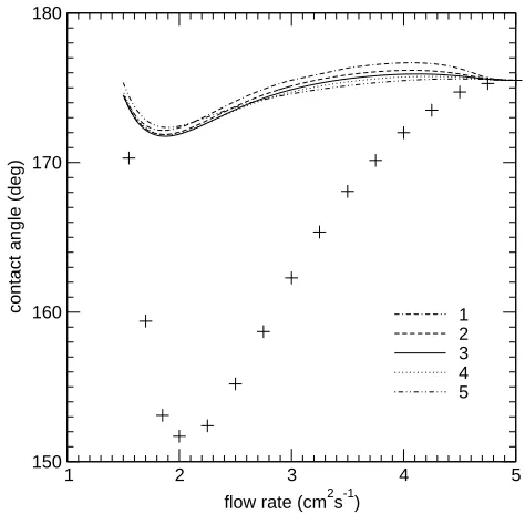
The results of the calculations are shown in Figs. 3–6, where we compare theoretical curves with the experimen-tal data from Fig. 2 corresponding toU = 70 cm s−1_.

For these results, the capillary number Ca ≡µU/σ = 0.273 and the Reynolds number, Re≡Q/ν, varies from 7.11 to 23.7 (here σ is the surface tension, ν the kine-matic viscosity, andQ the flow rate). The values of θd

prescribed in each case for the apparent contact angle to match the experimental one at high flow rates are given in Tables I and II for the slip models (2) and (4), respec-tively. Comparison with the other experimental curves from Fig. 2 gives results similar to those shown in Figs. 3– 6.

As is clear from the figures, in all cases the changes in the apparent contact angle are too small to account for the experimentally observed effect of the flow field vari-ation on the contact angle. The discrepancy cannot be attributed to experimental errors given that, as reported in Ref. [1], even in a single measurement the typical ac-curacy of determining the contact angle was about±5◦_,

whereas the data in Fig. 2 obtained after averaging over multiple measurements was significantly less than that.

5

1 2 3 4 5

flow rate (cm2s-1) 150

160 170 180

contact angle (deg) ₁

2 3 4 5

FIG. 3: Variation ofθapp1with flow rate for the model using

a prescribed (exponential) slip-velocity distribution (2) with various slip lengths. Curves 1, 2, 3, 4 and 5 correspond to

s1 = 0.01, 0.1, 1, 10, 100µm, respectively. The experimental

data (+ + +) are taken from Fig. 2,U = 70 cm s−1_.

TABLE I: The values of θd required to match the

“appar-ent” contact angles, θapp1 and θapp2, to the experimentally

measured contact angle (175.5◦_{, flow rate: 5 cm}2_s−1_{) for a}

slip model with the exponential velocity distribution (2) and

various slip lengths,s1.

s1 (µm) θdforθapp1 θdforθapp2

0.01 166.80 169.18

0.1 170.55 172.15

1.0 173.25 174.15

10.0 174.93 175.37

100.0 175.81 176.31

given in Figs. 3–6. One can also see from Figs. 3–6 that in all cases the magnitude of the apparent contact angle variation saturates as the slip length decreases, and the theoretical curves become practically undistinguishable from one another at smaller slip lengths. Further reduc-tion of the slip length reverses the trend and the curves become more shallow. Thus, for a given distance OA (Fig. 1), which corresponds to the (known) spatial reso-lution of the measurements [1], in the whole range of slip lengths,s1, or the values of the coefficient of sliding fric-tion, β, neither “apparent” contact angle describes the behaviour of the experimental data. It should be noted that there are no more parameters in the slip models which would allow one to improve the fit.

The same conclusions also follow from an attempt to fit a theoretical curve to the data using the resolution (the distance OA, Fig. 1) as an adjustable parameter. Our calculations show that to make the “apparent” contact

1 2 3 4 5

flow rate (cm2s-1) 150

160 170 180

contact angle (deg) ₁

2 3 4 5

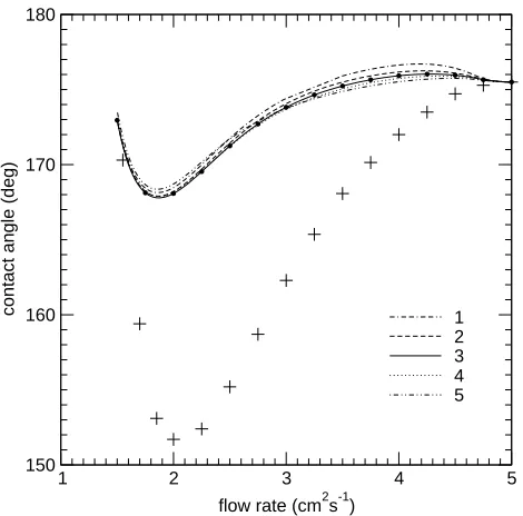
FIG. 4: Variation ofθapp1with flow rate for the model using

the Navier condition (4) with various coefficients of sliding

friction. Curves 1, 2, 3, 4 and 5 correspond toβ= 1000, 100,

10, 1, 0.1 kg/(cm2_{s), respectively. The experimental data (+}

+ +) are taken from Fig. 2,U = 70 cm s−1_.

TABLE II: The values ofθd required to match the

“appar-ent” contact angles, θapp1 and θapp2, to the experimentally

measured contact angle (175.5◦_{, flow rate: 5 cm}2_s−1_{) for a}

slip model with the Navier condition (4) with various values

of the coefficient of sliding friction,β.

β(kg cm−2_s−1₎

θdforθapp1 θdforθapp2

1000.0 165.33 167.90

100.0 167.03 169.30

10.0 168.98 170.77

1.0 170.95 172.24

0.1 173.05 173.92

angle variation close to that of the observed contact angle the resolution has to be about 150µm, i.e. about half the curtain thickness. This requirement is clearly beyond any reasonable interpretation of the measurements, as one can conclude simply by looking at the photograph of the curtain coating experiment, Fig. 4 in Ref. [1].

Thus, the simple arguments based on the order-of-magnitude analysis advanced by Blakeet al.[1] are con-firmed quantitatively, and one can assert that the influ-ence of the flow field/geometry on the dynamic contact angle cannot be attributed entirely to bending of the free surface under the changing hydrodynamic stresses. At a fixed contact-line speed, the flow field variations caused by other factors do affect theactual contact angle.

1 2 3 4 5 flow rate (cm2s-1)

150 155 160 165 170 175 180

contact angle (deg) ₁

2 3 4 5

FIG. 5: Variation ofθapp2with flow rate for the model using

a prescribed (exponential) slip-velocity distribution (2) with various slip lengths. Curves 1, 2, 3, 4 and 5 correspond to

s1 = 0.01, 0.1, 1, 10, 100µm, respectively. The experimental

data (+ + +) are taken from Fig. 2,U = 70 cm s−1_.

1 2 3 4 5

flow rate (cm2s-1) 150

160 170 180

contact angle (deg) ₁

2 3 4 5

FIG. 6: Variation ofθapp2with flow rate for the model using

the Navier condition (4) with various coefficients of sliding

friction. Curves 1, 2, 3, 4 and 5 correspond to β = 1000,

100, 10, 1, 0.1 kg/(cm2_{s), respectively. The experimental}

data (+ + +) are taken from Fig. 2, U = 70 cm s−1_{. The}

black circles are data obtained in a repetition of the curve 3 calculation made using a mesh approximately twice as dense as the original.

other words, by acontinuous set of data. Therefore, the description of the flow field cannot in principle be reduced to afinite (or even countably infinite) number of hydro-dynamic factors, which could be put as arguments on the right-hand side of Eq. (5). Thus, the very functional form of Eq. (5) appears to be inadequate for modelling flows associated with moving contact lines in a general flow geometry. For a given liquid-solid system, the contact angle is not merely a function of the contact-line speed (and a number of other hydrodynamic factors); it is a

functional of the flow field. In other words, the contact angle θd must be part of the solution. We will briefly discuss this issue in the next section.

A conclusion to be drawn from the tables is that in all cases θd is far from the static contact angle, θs: in the experimentsθs = 67◦_{. Thus, our results do not support}

the assumption that θd ≡ θs when the contact line is moving, which is used in a number of works [8, 16, 18– 23]. This assumption needed the ad hoc concept of an “apparent” contact angle to describe the behaviour of the experimentally observed contact angle with the ra-tio of the resolura-tion to the slip length as an adjustable parameter to fit the theory to the data. This approach was widely used for almost two decades, but gradually it became clear [5, 17] that even in treating the veloc-ity dependence of the observed contact angle in standard pipe-flow experiments the assumption thatθd≡θsmust be abandoned. The experiments of Blake et al. [1] and our calculations in the present paper provide a more gen-eral understanding of the reasons for that. Indeed, it was shown that θd depends on the flow field and, since the contact-line speed is the main factor influencing the flow field near the moving contact line, it will makeθddeviate fromθseven for what are, in other respects, similar flow conditions.

VI. CONCLUSIONS

Our results show the following:

1). Bending of the free surface in the vicinity of the contact line and the resulting deviation of the so-called “apparent” contact angle from the actual one do not describe the effect observed in the experi-ments [1].

2). Therefore one has to conclude that, for a fixed contact-line speed, variations of the flow field in the vicinity of the moving contact line caused, for example, by other closely located boundaries do influence the actual dynamic contact angle, that is the angle which has to be used as a boundary condition in the fluid dynamical modelling of dy-namic wetting. This effect cannot be described in the framework of the conventional approach to the moving contact line problem summarized in Sec. II.

7

to the static (equilibrium) contact angleθs, as sug-gested, for example, in [22], nor, as is sometimes assumed [24, 25], to 180◦_.

Thus, it has been shown that the conventional approach to the moving contact-line problem, which uses the func-tional form of Eq. (5) to determine the actual contact an-gle, is irreparably flawed and a different one is required. At present, the only known theory that makesθd part of the solution and hence dependent on the bulk flow is the one developed in [11] and briefly recapitulated in [1]. This theory considers dynamic wetting as a particu-lar case of a more general physical phenomenon, i.e. the fluid motion with formation/disappearance of interfaces. Since dynamic wetting is, by its very name, the process of creating a new — ‘wetted’ — solid surface, i.e. a fresh liquid-solid interface, it is clear that the surface proper-ties of this interface, such as the surface tension, have to relax from some dynamic values at the contact line to their equilibrium values away from it. The surface-tension-relaxation process depends on the rate at which the bulk flow creates the free interface and, due to the resulting surface-tension gradient, has a reverse influence on the bulk flow. The dynamic surface tensions at the contact line ‘negotiate’ the appropriate value ofθdto sat-isfy the (dynamic) Young equation, which represents the balance of forces acting on the contact line and replaces Eq. (5) one has in the slip models. The contact angle provides the boundary condition needed to determine the shape of the free surface and hence has a reverse influence on the bulk flow. As a result, the bulk flow, distributions of the surface tensions along the interfaces in the vicinity of the moving contact line and the value of the contact angle all become interdependent, and they all have to be found simultaneously as a solution to the correspond-ing mathematical problem. This problem is much more challenging mathematically than the one considered in the present paper and it will be addressed in a future work. The main question remains the same: is it possible to describe the data from [1] quantitatively with realistic values of the parameters involved? Preliminary estimates show that the key parameter determining the effect is the ratio of the length scale over which the surface tension relaxes to its equilibrium value and the length scale as-sociated with the Stokes regime near the moving contact line. However, these qualitative conclusions are yet to be verified quantitatively.

It should also be mentioned that the experimental ob-servations reported by Blakeet al.[1] have recently been corroborated independently [26] using an improved ap-paratus. The key qualitative features that seem to have led to the observed dependence of the contact angle on the flow geometry are: (a) a relatively high wetting speed and (b) a sufficiently small length scale characterizing the variation of the flow field allowed by the curtain coat-ing set-up. Recently, it has been shown experimentally [27] that in another flow configuration, namely that of an impacting drop, the observed contact angle also de-pends, besides the contact-line speed, on the flow field

in the vicinity of the contact line. Together with the results of Refs. [1, 26] this suggests that the nonlocal hydrodynamic influence on the contact angle is a generic phenomenon and more research into it is required to in-vestigate the effect of different fluid/solid combinations as well as various flow configurations.

APPENDIX A: COMPUTATIONAL DETAILS

The governing equations for the simulations presented here are the dimensionless Navier-Stokes equations ap-propriate for an isothermal incompressible Newtonian liquid of density ρ, viscosity µ, and surface tension σ

experiencing a gravitational acceleration ofg:

Reu.∇u = ∇.T+ (Bo/Ca)ˆg, (A1)

∇.u = 0, (A2)

whereu = (u, v) is velocity,ˆg is a unit vector indicating the direction of gravity, andT is the stress tensor with componentsTαβ=−pδαβ+∂uα/∂xβ+∂uβ/∂xα(pbeing the pressure). The velocity is scaled by the substrate speed, U, while lengths are scaled by the coated film thickness, Q/U (where Q is the flow rate), and stresses are scaled byµU2_{/Q. The Reynolds, capillary and Bond}

numbers are therefore given byRe=ρQ/µ,Ca=µU/σ, andBo=ρgQ2_/σU2 _{respectively. The numerical values}

ofReandCaare given in Sec. V; the Bond number varies from 8.34×10−3 _{to 0.093.}

We solved Eqs. (A1) and (A2) numerically using a Galerkin, weighted residual finite element formulation in which the domain is tessellated using Taylor-Hood tri-angular elements featuring six velocity nodes and three pressure nodes. Such elements satisfy the LBB stability condition [28] and, with the pressure interpolation one order lower than that of velocity, no ‘locking’ occurs [29]. The general approach is well-established in the field of coating flow simulation [30] so only a brief description is given here.

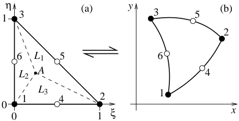
The algebraic finite element equations are derived in terms of a right-angled ‘master’ element, which has local coordinates (ξ, η) as shown in Fig. 7(a). Within this ele-ment the velocity and pressure are expressed in terms of their nodal values,ui,pj, by means of biquadratic (Qi)

and bilinear (Lj) interpolation functions:

u(ξ, η) =

6

X

i=1

uiQi(ξ, η); p(ξ, η) =

3

X

j=1

pjLj(ξ, η).

(A3) With reference to Fig. 7(a) it is easy to see that the three linear functions are given by

L1= 1−ξ−η, L2=ξ, and L3=η,

A L1

L2

ξ x

y

4 6

1

(b) (a)

1 4

6

3 ₅

2

L

1

0

0 1

2 5

3 3 η

FIG. 7: (a) The ‘master’ element, with local coordinates

(ξ, η), which is used to derive the finite element equations.

The numbered black circles represent nodes at which velocity and pressure values are to be found, while the white circles are velocity-only nodes. The areas of the subtriangles formed

by connecting pointA to the vertices give, when divided by

the total area of the element, the values of the linear

inter-polation functions Lj at point A. (b) A general element in

physical space; the master element is mapped into each phys-ical element by means of the quadratic transformation (A4).

property with respect to the six velocity nodes. The Qi

are also used to map the master element in local space into each general curved element in global (x, y) = x

space (Fig. 7b) via the transformation

x(ξ, η) =

6

X

i=1

xiQi(ξ, η), (A4)

wherexi= (xi, yi) are the global coordinates of the

ele-ment’s nodes. The formulation of the weighted residual equations is completed by substituting Eqs. (A3) into Eqs. (A1) and (A2), weighting these by Qi and Lj re-spectively, integrating over the entire domain, Ω, and requiring the resulting expressions to vanish. After some manipulation using vector identities and the divergence theorem, the equations to be solved become

Z

Ω

[QiReu.∇u + ∇Qi.T−Qi(Bo/Ca)ˆg]dΩ

−

Z

∂Ω

Qinˆ.Tds= 0 (A5)

and

Z

Ω

Lj∇.udΩ = 0, (A6)

where dΩ =dxdy, nˆ is a unit normal to the boundary,

∂Ω, of the domain, andsis arc length along the bound-ary.

The boundary conditions for the problem are as fol-lows. On the (stationary) walls of the slot feeding the curtain (Fig. 1), the no-slip condition is applied. On the substrate being coated, either the Navier condition, Eq. (4), or an exponential velocity distribution, Eq. (2), is applied (see Sec. II) along with the impermeability con-ditionv= 0. On the free surfaces we have the kinematic

condition,

ˆ

n.u = 0, (A7)

together with (a) the condition of zero tangential stress (the viscosity of the ambient gas being negligible) and (b) the balance of normal stress with capillary pressure. Mathematically, conditions (a) and (b) are encapsulated in the form [31]

ˆ

n.T = 1

Ca

dˆ_t

ds, (A8)

whereˆ_{t is the unit tangent to the free surface. This can}

be inserted directly into Eq. (A5) and, after integrating by parts, the boundary integral becomes

Qi

Ca[ˆtE−ˆtB]−

1

Ca

Z

∂ΩF S

ˆ_tdQi

ds ds, (A9)

whereˆ_{tB and}ˆ_{tE are the unit tangents to the beginning}

and end of the free surface respectively, and∂ΩF S

repre-sents the free surface part of the domain boundary. The remaining boundary conditions are a parabolic velocity profile imposed at the top of the feed slot, a uniform ve-locity profile imposed where the film leaves the domain, and the condition that the upstream free surface meets the substrate at an angle equal toθd.

The free surface parametrization is based on the ‘spine’ approach developed by Kistler and Scriven [31, 32]. The essence of the method is that each node on a free surface is constrained to lie along one of a set of conveniently de-fined lines or curves (known as ‘spines’) which intersect the free surface. For example, a simple linear spine (num-beredi, say) is defined by its base point, bi, which may

be fixed or may lie on another spine, and its unit direc-tion vector,ˆei. The free-surface node lying on this spine

is then located atx =bi+hiˆei, i.e. a distancehi along

the spine from its base point. Between the free-surface nodes the shape of the free surface is given via the curved edges of the elements which lie along the surface, i.e. by Eq. (A4). Hence the free surface is represented by a piece-wise quadratic curve. Nodes in the interior of the domain are positioned along the spines according to some suit-able (often uniform) distribution, e.g.xj =bi+wjhiˆei.

The set of allhi then forms a set of parameters which completely describes the free surfacesand allows the in-terior mesh to deform in response to deformations of the free surfaces. The unknownhiare determined by forming a weighted residual from Eq. (A7), i.e. by solving

Z

∂ΩF S

Qiˆn.uds= 0. (A10)

9

E

B

R

h

h

A

D

C

fixed

fixed

O

O

d

feed slot

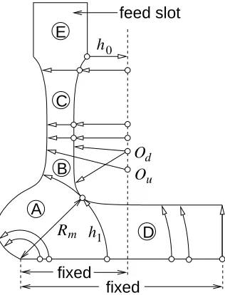
FIG. 8: The system of linear and circular spines used to parametrize the free surfaces. Spine base points are shown as circles. Regions A and D feature circular spines centered on the contact line; region B is represented in terms of linear

spines based at two polar origins, Ou andOd, with circular

arcs constructed between the free surfaces; region C’s spines are linear and horizontal; and region E is the feed slot, where the mesh is fixed.

complete spine system is illustrated in Fig. 8. The cir-cular spines are defined by a centre point (in most cases the contact line), a radius, and a base point; the pa-rameter hi for these spines is then the angle subtended at the centre point by the base point and the relevant free surface node. The most important spine in Fig. 8 is

h0, which tethers the contact line (and indeed the entire free-surface mesh) to the fixed wall of the feed slot by defining the location of the vertical baseline shown in the diagram. The value of h0 (i.e. the length of the spine) is determined from the condition that the upstream free-surface must meet the solid substrate at an angle ofθd. Other important quantities upon which mesh regions A, B and D depend are the angle of the circular spineh1and the associated radial distanceRm which together locate the point on the downstream free surface which is closest to the contact line. The radii of the circular spines in regions A and D are given as fractions or multiples of

Rm.

The spine system in Fig. 8 enabled the same mesh structure to be used under both low and high flow rate conditions, see Fig. 9. For high flow rates, additional strips of elements were simply inserted to maintain mesh quality. Close to the dynamic contact line, the density of the mesh was chosen so that the large velocity gradients on the solid surface were sufficiently well-represented. Hence the size of the elements in the slip region was at least an order of magnitude smaller than the slip length scale. Near the contact line the mesh must also be suit-ably fine in the aziumthal direction in order to capture

(b)

(c)

(a)

FIG. 9: Part of the computational mesh showing the node dis-tribution for (a) the low flow rate limit, (b) a typical medium flow rate, and (c) the high flow rate limit. Note that the meshes are not shown on the same scale.

-5 -4 -3 -2 -1 0 1 2 3 4 5

(×10-5) 0

1 2 3 4 5

(

×

10

-5 )

FIG. 10: A close-up view of the mesh near the contact line,

formed by magnifying Fig. 9(b) by a factor of 105_{. The}

co-ordinates on the axes are in units of coating film thickness,

which in this case is 428µm.

the velocity field with sufficient accuracy. A close-up of the mesh near the contact line is given in Fig. 10. The density of the rest of the mesh was adequate for further refinements to produce only negligible changes to the so-lution. As an illustration of the effect of mesh density, Fig. 6 includes (as black circles) the results from a re-peat of the β = 10 kg cm−2_s−1 _{(curve 3) calculations}

made using meshes with approximately twice the node density of those used to generate curve 3. The results are indistinguishable on the scale of the graph.

to zero, one has

p= βU

θd lnr+. . . , (A11)

whereas the stream function in local polar coordinates has the formψ=U r2_{F(θ), where}

F(θ) =B1+B2θ+B3sin 2θ+B4cos 2θ,

with

B1=−B4=−βl

4µ, B2=−

1

θdB1, B3=B1cot(2θd),

and this generates a regular flow field. (Herer is scaled as above by Q/U.) Since the pressure singularity in Eq. (A11) is integrable, it has been ignored in the compu-tations reported in the literature, and the pressure over the elements comprising the contact line was approxi-mated in the same way as in the bulk (described above). However, the computational mesh necessarily includes a pressure node located at the contact line. Since the so-lution cannot return the correct (i.e. negatively infinite) value of pressure at this node, it is desirable to redefine the pressure interpolation on the elements touching the contact line so as to avoid having a finite pressure at this point and hence to obtain a uniformly valid solution.

Following Suckling [33], to cope with the singular pres-sure field at the contact line, the linear prespres-sure interpola-tion funcinterpola-tions in the elements adjacent to the contact line were augmented with logarithmic functions correspond-ing to Eq. (A11). Consider Fig. 7(a) in the context of an element adjacent to the contact line. The numbering system employed in the computational mesh is chosen so that local node 1 corresponds to the contact line. Using Eq. (A4), we therefore have

r(ξ, η) =|x −x1| =



 Ã ₆

X

i=1

{xiQi(ξ, η)} −x1

!2

−

à 6

X

i=1

{yiQi(ξ, η)} −y1

!2



1/2

(A12)

and the logarithmic singularity can be incorporated by replacing interpolation functionL1by

L∗1=L1lnr= (1−ξ−η) lnr. (A13)

The pressure is then given by

p(ξ, η) =p1L∗1+p2L2+p3L3.

Note that L∗

1 vanishes along the element edge opposite

the contact line (between nodes 2 and 3), and therefore the augmented elements are completely compatible with the regular elements used in the bulk of the domain. As node 1 is approached, i.e. as ξ, η → 0 and hence

r→0, however,L∗

1 provides the correct functional form

(x 10 )

(x 10 )

−5

−5

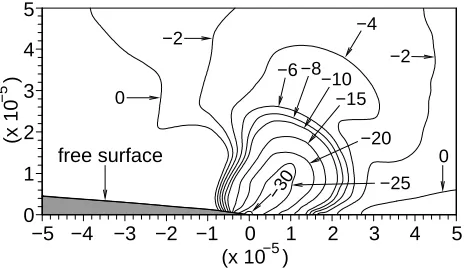
−5 −4 −3 −2 −1 0 1 2 3 4 5 0 1 2 3 4 5 −2 −15 −20 −25 −8 −10 −6 −30 free surface −4 0 0 −2

FIG. 11: Typical dimensionless pressure contours in the vicin-ity of the dynamic contact line. The field of view covers

the same area as Fig. 10. In this caseQ = 3 cm2_s−1 _and

θd = 169◦. Note that the contour labels show multiples of

1000.

to match Eq. (A11). Importantly, using this approach,

p1 no longer represents a finite (and therefore incorrect) value of pressure at the contact line, but instead provides the coefficient multiplying lnr.

The integration of the residual equations (A5), (A6) and (A10) is achieved on an element-by-element basis using the master element and transformation (A4), and the pressure gradient terms in the Navier-Stokes equa-tions give rise to integrals over the master element of the form

Z Z

pjLj(ξ, η) µ_∂Qi ∂ξ ∂y ∂η − ∂Qi ∂η ∂y ∂ξ ¶ dξdη (A14) and Z Z

pjLj(ξ, η) µ_∂Qi ∂η ∂x ∂ξ − ∂Qi ∂ξ ∂x ∂η ¶ dξdη, (A15)

where∂y/∂η etc. are found from Eq. (A4). Away from the contact line, the integrands are polynomials inξand

η(as are those arising from the other terms in the Navier-Stokes equations) and the integration of all terms is per-formed numerically by means of Gaussian quadrature. However, insertion of Eq. (A13) into integrals (A14) and (A15) — and indeed the continuity equation, where it also appears — produces integrands which are not regular polynomials, and therefore standard Gaussian quadra-ture is not appropriate for calculating these integrals. Another issue is that Eq. (A13) of course cannot be eval-uated at the contact line itself. To enable the calcula-tion of these integrals, a small region of radiusǫaround node 1 is excluded from the master element, and a re-cursive adaptive Simpson’s rule quadrature is used to in-tegrate over the remainder of the element. Suckling [33] showed that the error in excluding the contact line region isO(ǫ2_{lnǫ) asǫ →0, and tested the quadrature}

gener-11

ating the results presented in this paper. A plot of the pressure field close to the contact line is given in Fig. 11. Note that the singularity in the pressure field also gives rise to a corresponding integrable singularity in the free-surface curvature at the contact line, though the con-tact angle remains well-defined. Unlike the pressure field, however, the singularity in curvature does not require any special treatment since the normal and tangential stress conditions are imposed in integral form, see Eq. (A8), and therefore the only requirement for a uniformly convergent

solution is that the curvature should be integrable, which it is. The fact that the free-surface discretization is suf-ficient is demonstrated by the mesh-independence of the results (see Fig. 6).

Finally, the residual equations were solved using New-ton iteration in which the Jacobian at each iteration was inverted by the frontal method [34]. The iterative pro-cess was terminated when theL2 norm of the residuals fell below 10−8_{; typically 4–8 iterations were needed to}

satisfy this criterion.

[1] T. D. Blake, M. Bracke, and Y. D. Shikhmurzaev, Phys.

Fluids 11, 1995 (1999).

[2] T. D. Blake, A. Clarke, and K. J. Ruschak, AIChE J.40,

229 (1994).

[3] R. J. Hansen and T. Y. Toong, J. Colloid Interf. Sci.36_,

410 (1971).

[4] Y. D. Shikhmurzaev, J. Fluid Mech.334, 211 (1997).

[5] M. Y. Zhou and P. Sheng, Phys. Rev. Lett. 64_{, 882}

(1990).

[6] P. Sheng and M. Zhou, Phys. Rev. A45, 5694 (1992).

[7] D. E. Finlow, P. R. Kota, and A. Bose, Phys. Fluids 8_,

302 (1996).

[8] E. B. Dussan V., J. Fluid Mech.77, 665 (1976).

[9] M. Navier, Mem. Acad. Sci. Inst. Fr. pp. 389–440 (1823).

[10] H. Lamb,Hydrodynamics(Dover, New York, 1932).

[11] Y. D. Shikhmurzaev, Int. J. Multiphase Flow 19, 589

(1993).

[12] R. A. Hayes and J. Ralston, J. Colloid Interf. Sci. 159_,

429 (1993).

[13] R. L. Hoffman, J. Colloid Interf. Sci.50, 228 (1975).

[14] C. G. Ngan and E. B. Dussan V., J. Fluid Mech.118_{, 27}

(1982).

[15] P. Bach and O. Hassager, J. Fluid Mech.152, 173 (1985).

[16] R. G. Cox, J. Fluid Mech.168_{, 169 (1986).}

[17] M. Fermigier and P. Jenffer, J. Colloid Interf. Sci. 146,

226 (1991).

[18] L. M. Hocking and A. D. Rivers, J. Fluid Mech.121_{, 425}

(1982).

[19] C. Huh and S. G. Mason, J. Fluid Mech.81, 401 (1977).

[20] L. M. Hocking, J. Fluid Mech.79_{, 209 (1977).}

[21] L. M. Hocking, Q. J. Mech. App. Math.34, 37 (1981).

[22] L. M. Hocking, J. Fluid Mech.239_{, 671 (1992).}

[23] P. A. Durbin, J. Fluid Mech.197, 157 (1988).

[24] V. V. Pukhnachev and V. A. Solonnikov, PMM — App.

Math. & Mech.46, 961 (1982).

[25] C. Baiocchi and V. V. Pukhnachev, J. Appl. Mech. Techn. Phys. (USSR) pp. 27–40 (1990).

[26] A. Clarke and E. Stattersfield, Phys. Fluids, submitted (2006).

[27] ˇS. ˇSikalo, H.-D. Wilhelm, I. V. Roisman, S. Jakirli´c, and

C. Tropea, Phys. Fluids17, 062103 (2005).

[28] I. Babuska and A. K. Aziz, inMathematical Foundations

of the Finite Element Method with Applications to Partial Differential Equations, edited by A. K. Aziz (Academic Press, New York, 1972), pp. 1–135.

[29] T. J. R. Hughes, The Finite Element Method: Linear

Static and Dynamic Finite Element Analysis (Prentice-Hall, 1987).

[30] S. F. Kistler and P. M. Schweizer,Liquid Film Coating:

scientific principles and their technological implications (Chapman and Hall, 1997).

[31] S. F. Kistler and L. E. Scriven, inComputational Analysis

of Polymer Processing, edited by J. R. A. Pearson and S. M. Richardson (London & New York: Applied Science, 1983), pp. 243–299.

[32] S. F. Kistler and L. E. Scriven, Int. J. Num. Meth. Fluids

4, 207 (1984).

[33] P. M. Suckling, Ph.D. thesis, University of Birmingham (2003).