Application of a portable FTIR for measuring on-road emissions

This is a repository copy of Application of a portable FTIR for measuring on-road

emissions.

White Rose Research Online URL for this paper:

http://eprints.whiterose.ac.uk/2043/

Book Section:

Daham, Basil, Andrews, Gordon E., Li, Hu et al. (4 more authors) (2005) Application of a

portable FTIR for measuring on-road emissions. In: SAE Book SP-1941: Emissions

Measurement and Testing 2005. Society of Automotive Engineers , USA , pp. 171-192.

ISBN 0-7680-1586-32005

SAE Paper # 2005-01-0676

[email protected] https://eprints.whiterose.ac.uk/

Reuse

See Attached

Takedown

If you consider content in White Rose Research Online to be in breach of UK law, please notify us by

400 Commonwealth Drive, Warrendale, PA 15096-0001 U.S.A. Tel: (724) 776-4841 Fax: (724) 776-5760 Web: www.sae.org

2005-01-0676

Application of a Portable FTIR for

Measuring On-road Emissions

Basil Daham, Gordon E. Andrews, Hu Li, Rosario Ballesteros,

Margaret C. Bell, James Tate and Karl Ropkins

University of Leeds, UK

Reprinted From: Emissions Measurement and Testing 2005

(SP-1941)

2005 SAE World Congress

Detroit, Michigan

April 11-14, 2005

SAE TECHNICAL

The Engineering Meetings Board has approved this paper for publication. It has successfully completed SAE’s peer review process under the supervision of the session organizer. This process requires a minimum of three (3) reviews by industry experts.

All rights reserved. No part of this publication may be reproduced, stored in a retrieval system, or transmitted, in any form or by any means, electronic, mechanical, photocopying, recording, or otherwise, without the prior written permission of SAE.

For permission and licensing requests contact:

SAE Permissions

400 Commonwealth Drive

Warrendale, PA 15096-0001-USA Email: [email protected] Tel: 724-772-4028

Fax: 724-772-4891

For multiple print copies contact:

SAE Customer Service

Tel: 877-606-7323 (inside USA and Canada) Tel: 724-776-4970 (outside USA)

Fax: 724-776-1615

Email: [email protected]

ISSN 0148-7191

Copyright © 2005 SAE International

Positions and opinions advanced in this paper are those of the author(s) and not necessarily those of SAE. The author is solely responsible for the content of the paper. A process is available by which discussions will be printed with the paper if it is published in SAE Transactions.

Persons wishing to submit papers to be considered for presentation or publication by SAE should send the manuscript or a 300 word abstract to Secretary, Engineering Meetings Board, SAE.

ABSTRACT

The objective of this work was the development of an on-road in-vehicle emissions measurement technique utilizing a relatively new, commercial, portable Fourier Transform Infra-Red (FTIR) Spectrometer capable of identifying and measuring (at approximately 3 second intervals) up to 51 different compounds. The FTIR was installed in a medium class EURO1 spark ignition passenger vehicle in order to measure on-road emissions. The vehicle was also instrumented to allow the logging of engine speed, road speed, global position, throttle position, air-fuel ratio, air flow and fuel flow in addition to engine, exhaust and catalyst temperatures. This instrumentation allowed the calculation of mass-based emissions from the volume-mass-based concentrations measured by the FTIR. To validate the FTIR data, the instrument was used to measure emissions from an engine subjected to a real-world drive cycle using an AC dynamometer. Standard analyzers were operated simultaneously for comparison with the FTIR and the standard analyzer results showed that most pollutants (NOx, CO2, CO) were within ~10% of a standard analyzer during steady state conditions and within 20% during transients. The exception to this was total HC which was generally 50% or less than actual total HC, but this was due to the limited number of hydrocarbons measured by the FTIR. In addition to the regulated emissions, five toxic hydrocarbon species were analyzed and found to be sensitive to cold starts in varying proportions. Finally, FTIR data was compared to results from a commercially available on-road measurement system (Horiba OBS-1000), and there was good agreement.

INTRODUCTION

In Europe there is a requirement for all cities to monitor and model their urban air quality. If European air quality

targets are not met then action must be taken and in virtually every case of non-compliance, traffic-related pollution is responsible, especially in urban or industrialized areas [1-4]. To model urban air pollution, the mass emissions of road transport have to be modeled together with their dispersion. Traffic movement and emissions needs to be modeled on a second-by-second basis for incorporation in an air dispersion model that calculates the amount of pollutants present based on actual meteorological factors. To provide the dispersion model with emission data, the traffic model needs accurate information on the emissions of cars under different driving conditions. Normally this data is derived from legislated test cycle emissions data by applying various correction factors for speed. To improve the accuracy of these air pollution models, it is preferable to measure on-road vehicle emissions instead of deriving them from the legislated drive cycle data which may not be representative of real traffic conditions. Car manufacturers are continuously improving the emissions of their vehicles, especially with the latest EURO4 legislation in Europe. On-road testing is not part of the legislative process and therefore a vehicle is only subjected to the mild ECE15 drive cycle in Europe, and the slightly more aggressive FTP75 in the USA. It is not a legal requirement for the vehicle to maintain clean exhaust emissions outside the operating conditions needed to negotiate these standard drive cycles. Therefore a vehicle driven in real-world conditions where situations might require hard acceleration might not meet the legislated standards. Real-world on-road testing helps to ascertain this possibility.

It is widely accepted that legislated drive cycles such as the FTP75 and ECE15 underestimate emissions from cars under real-world conditions [5-9]. This is especially true for CO and HC but less so for NOx [10,11]. Vogel et al. [10] found that CO emission factors were increased by a factor of two in real life. De Vlieger’s [11] results

2005-01-0676

Application of a Portable FTIR for

Measuring On-road Emissions

Basil Daham, Gordon E. Andrews, Hu Li, Rosario Ballesteros

Margaret C. Bell, James Tate and Karl Ropkins

Copyright © 2005 SAE International

were more extreme having determined CO to be four times, and HC+NOx to be twice, the legislated levels for a EURO1 vehicle in real-world driving. Real-world emissions depend on many factors such as driving behavior, traffic conditions, weather and ambient temperature conditions, vehicle model, fuel used, traffic conditions and network geometry [6]. Hence it is unrealistic to predict atmospheric pollution from emission factors obtained from the standardized legislated drive cycles. Correction factors may be applied for various parameters but in the end it is much better to measure actual real-world emissions in real traffic flow conditions Also, if a city is to reduce emissions from traffic in order to control the air quality, it needs to know how emissions will be reduced as a result of traffic management measures. In-vehicle emissions measurement in real traffic conditions allows the impact of different traffic management measures on emissions to be directly determined.

The techniques developed in this study aim to address the shortcomings of rolling road dynamometer testing as conducted by most laboratories and emissions legislation bodies. The main limitations imposed by the use of a rolling road dynamometer are the limited acceleration rates possible (due to tire slippage) and the limited air flow rate around the car. In addition to the advantage of measuring exhaust emissions under real-world driving conditions, the technique also potentially permits the partial speciation of the emitted hydrocarbons so that toxic hydrocarbons such as benzene and 1,3-butadiene can be determined. The ability to measure individual HC components allows the calculation of the ozone forming potential (OFP) of the vehicle’s emissions as well as indicating if any of the individual hydrocarbons are above any allowable health and safety limits.

PREVIOUS DESIGNS

The following is a literature review of the systems that have been proposed and used in the past for measuring real-world emissions.

REMOTE SENSING

Remote sensing was once considered by the EPA as the solution to the transport pollution problem. The plan was to install remote sensors across the US highways together with number plate recognition cameras and then issue fines to the polluting vehicles based on the amount of pollutants being produced. This was all too ambitious since this technique simply provides a ‘snapshot’ of the emissions of the vehicle in question as it passes through the remote sensor. This is obviously not an indication of the average level of emissions being produced by the vehicle and therefore it would be unfair to issue any fine based on this one ‘snapshot’ of emissions. The driver of an offending vehicle could simply let off the throttle as they passed through the sensor in order to avoid detection.

For determining emissions factors from road traffic in a Switzerland tunnel, Staehelin et al. [12] measured NOx, CO and THC’s at 5-minute intervals at the tunnel entrance and exit simultaneously. They also measured semi-volatile hydrocarbons using a GC-type Airmotec HC 1010 at 15-minute intervals. Air flow rate through the tunnel was measured with a Flowsic 400. Tracer SF6 gas was injected at the tunnel entrance and then used to evaluate tunnel ventilation as well as the level of turbulent mixing at the tunnel exit using six sampling points on the periphery. Vehicle speed was also monitored in addition to the license plates. This tunnel study was one week long and provided information on tunnel ventilation as well as the necessary emissions factors to be used in air pollution prediction models.

In another 20-day remote sensing experiment, Vogel et al. [10] carried out a study on a stretch of German motorway to determine real-life emissions and compare those to data calculated from pollution models. VOC (Volatile Organic Compound) measurements were done by GC-MS at 55-minute intervals while NO, NOx, CO and O3 were averaged over 10 minutes. These measurements were done at various positions perpendicular to the highway (25m, 50m, 75m, 100m, 150m and 400m) and at various heights above the ground. It was found that pollution models correlated well (within error bars) with real-world measurements once the real traffic data (as opposed to modeled traffic data) was input into the models. The exception to this was CO where a discrepancy factor of two was found between real-world and predicted values.

ON-BOARD MEASUREMENTS

Hands et al. later modified this CO2 [15] sensor to make a fast response (7ms response time) CO sensor. Under rich cold-start conditions the CO sensor allows a faster estimate of stoichiometry than the UEGO sensor. It can also be used to monitor air-fuel ratio on the rich side. Using this CO sensor, differences in cylinder to cylinder air-fuel ratios were also identified. However these ultra-fast response instruments are not required for real-world measurement, where a 1-second response would be adequate.

De Vlieger [11] developed an on-board system that was used in a Belgium investigation of 6 cars, 3 road types and 3 driving behaviors. The system consisted of NDIR for CO and CO2, FID for THC’s, and CLD for NOx. These techniques are the measuring methods approved for legislation. Fuel consumption was accurately (1% within 0.5-60L/hr) measured. Exhaust flow rate was measured using the fuel consumption and calculated lambda value. Emission factor errors were within 10% for emissions compared to stationary equipment on a chassis dynamometer.

Honda and Nicolet also developed a system [16] that they used for measuring on-road emissions from a ZLEV (Zero Level Emissions Vehicle) car, which produces 1/10th the emissions levels of a ULEV (Ultra Low Emissions Vehicle) car. The system consists of two Nicolet FTIR detectors placed on the back seat of the car. One was used to sample intake air and the other sampled exhaust gases. It was shown in field tests [17] that the car was producing exhaust gases that were cleaner than the ambient intake air for some pollutants. The FTIR in this case was limited to measuring the gases of interest which were NMHC (Non-Methane HydroCarbons), NOx and CO. Another challenge was the development of techniques that allow a 0.1ppm limit of detection (LOD). Multi-tube Nafion dryers were used to remove the water from the exhaust since it was decided that spectral corrections for the water cross-interference necessitated a tedious calibration procedure and the accuracy would suffer if water was allowed to stay in the analysis. A cell with a 10m path length was chosen to attain the 0.1ppm LOD. Spectral resolution was 0.5cm-1 and CO2 cross interference was avoided by careful selection of analytical regions. The Mercury Cadmium Telluride (MCT) detector was cooled with liquid nitrogen for faster response. Cell pressure was kept constant at 700mmHg. It was found that the calculation of exhaust mass flow rate from the engine speed and fuel injection data was adequately accurate for the work [17]. Laboratory calibration was done in the ranges 0-2ppm Carbon, 0-20ppm CO and 0-2ppm NO. Excellent correlation was found between the FTIR-measured and actual propane, CO and NO. On the rolling road dynamometer, there was excellent agreement for CO and NO but not for NMHC since FID measures real THC’s. The project probably has little practical applicability outside Honda’s ZLEV since the measuring range is designed for a car producing ultra-low emissions.

Weaver et al. [18] developed the RAVEM (Ride-Along Vehicle Emission Measurement) system in order to accurately and repeatability measure NOx, CO2 and PM (Particulate Matter) on the road. The system is very much like the CVS (Constant Volume Sampling) system employed on rolling road dynamometers but it only samples a small fixed fraction of the total exhaust. To achieve proportionality, a stepper motor controls the throttle of the dilution air inlet based on pressure feedback signal from the exhaust probe thus making volume flow rate linearly proportional to the exhaust pipe flow rate. This is called isokinetic sampling and avoids the need for expensive equipment that measures the exhaust mass low rate. A FID was not used to measure THC’s since that would have required heated sample lines. Therefore the system is limited to measuring CO and CO2 by NDIR and NOx by heated CLD. PM was gravimetrically measured on pre-weighed 37mm Teflon-coated borosilicate glass fiber filter papers. This system was tested on a refuse truck and found to correlate well with a rolling road dynamometer for CO2, NOx and PM. However this equipment will not fit in a passenger car.

Kihara et al. [19] developed an on-board system that measures and logs NOx, fuel consumption and various other engine and vehicle parameters. Of note were the fast response ZrO2 sensors used to measure NOx (0-1000ppm) and air-fuel ratio (1-10λ). Fuel consumption was calculated from the inlet air mass flow meter and the inlet air conditions as well as the ZrO2 lambda sensor. The other sensors were conventional pressure transducers and thermocouples. This set-up was installed on the passenger seat of a diesel vehicle and was monitored for over a year. NOx emission patterns were found to correlate negatively with fuel economy. Seasonal influences on NOx emissions were noted, with NOx increasing during the lower humidity winter months. Compared to the standard CVS-bag method, the on-board system was found to be within 4% for NOx mass emission and 3% for fuel consumption. This same NOx sensor was used in the Horiba OBS-1000 system.

deemed too dangerous to install on-board due to the He/H2 bottle it requires. NOx was measured with a zirconium oxide (ZrO2) sensor and also verified with an electrochemical cell. Prior to drying the sample with a thermoelectric chiller, the sample gas was passed over a NOx converter. This was done since a large portion of the diesel NOx emissions is NO2 and the sensor only measures NO. A GPS system was used to record vehicle speed and verify it against the ECU output. Based on standard FTP tests, the MEMS was found to be within 5% of laboratory measurements when measuring brake-specific emissions.

Vojtisek-Lom et al. [21] developed a portable on-board system to be utilized in heavy duty vehicles. They used NDIR for CO and CO2, electrochemical cells for NOx and O2 and laser scattering detectors for PM. HC’s were not considered since it was believed that only a fraction of the exhaust HC’s reach the sample cell in gaseous form. Exhaust flow was calculated from engine operating data. Power consumption of the system was up to 15 Amperes and a backup battery capable of 1-minute power provision was also installed for cold starts. The sample line was 6m long, 6mm in diameter and unheated to avoid complexity and cost. Repeatability of the on-board system was found to be less than the bench equipment but fair correlation was established between on-board and bench measured NOx and CO2. Contrary to expectations, there were no problems with the response time of the electrochemical cells. PM measured on-board was validated against TEOM (Tapered Element Oscillating Mass) and gravimetric methods and the results were less than acceptable. More validation was recommended for the PM measurements. This system has been improved with HC analysis using NDIR [22].

PREVIEW (Portable Real-Time Emissions Vehicle Integrated Engineering Workstation) is an on-board emissions measuring system developed in-house by Ford and used by Nam et al. to calibrate an emissions model that provided output for use in a microscopic traffic model [23]. PREVIEW uses an NDIR for HC, CO and CO2, and a UV (UltraViolet) analyzer for NO. Wet sample gas is used, therefore necessitating heated cells, sample lines and a separate power supply. Engine and vehicle data were obtained directly from the PCM (Powertrain Control Module). The detection limits were 38ppm for CO, 10ppm for HC (as propane), 10ppm for NO and 200ppm for CO2, which means it would not be suitable for measuring low load conditions on a low emissions modern vehicle. The whole system weighed ~70kg and could be fitted on the back seat or in the trunk of a vehicle. Correlation with standard equipment on a dynamometer, using a 1997 sport utility vehicle driven over a US06 drive cycle, was very good.

Sensors Inc.’s previous experience helping Ford develop the PREVIEW system allowed it to develop the SEMTECH [24]. The SEMTECH-G (gasoline) and SEMTECH-D (diesel) were used by the EPA to generate data for facilitating the development and validation of a new generation of mobile emissions model called MOVES. The 36kg SEMTECH-D uses a heated

sampling system where the lines, filter and pump are kept at 195°C to avoid HC condensation. NDIR is used for CO and CO2, while a NDUV (Non Dispersive Ultraviolet) is used for NO and NO2. Engine and vehicle data is obtained from the vehicle data port directly and a GPS is used to track position and speed. The 20kg SEMTECH-G is similar to the diesel model but it uses NDIR for THC measurements, with the heated FID being optional. The reasoning behind this is that gasoline produces a lot of hexane which has strong infra-red absorbing properties and does not condense at ambient temperatures, A heated sampling system is not used in order to reduce power consumption. NDUV is used to only measure NO since NO2 is negligible in gasoline vehicles. Engine and vehicle data is obtained using the OBDII connector and a GPS is also used. Both systems are said to have a detection limit and uncertainty of 50ppm [24]. Correlation with rolling road dynamometer CVS is excellent.

Hawirko et al. developed an on-board emissions measurement system using a Vetronix PXA-1100 5-gas analyzer with a built-in sample handling system, a wide-band lambda sensor, a hot-wire Siemens mass air flow meter, and temperature probes for coolant, ambient and inlet temperatures [25], All parameters were logged on a laptop computer at an average of 1.5Hz along with engine and road speed. The analyzer used NDIR for HC, CO and CO2, and electro-chemical cells for NOx and O2. The system was later used to investigate the relationship between ambient temperature and emissions [26]. In this later study, 2- and 3-factor emission models were developed and compared to other one-factor emission models currently in use.

North et al. have developed an on-board emissions system called VPEMS (Vehicle Performance and Emissions Monitoring System) [27]. This uses a Nafion impregnated tube to dry the exhaust sample before introducing it into a commercially available 5-gas analyzer. This analyzer uses NDIR for CO, CO2 and HC, and electro-chemical cells for O2 and NOx. Engine and vehicle performance data is obtained from the CAN bus. On post-2001 European market cars this is possible via the standardized OBDII link, but on older cars it can be much harder. This data was then used to convert the concentration data from the analyzer into mass-based emissions. A GPS was incorporated and all sampling was done at about 1Hz. The VPEMS was referenced against a rolling road dynamometer CVS measure, and compensation factors were derived for all pollutants. Compared to bag results, the VPEMS aggregate mass emissions were off by 11% for CO, 8% for CO2 and 17% for NOx for the standard European drive cycle.

APPARATUS DESIGN

DESIGN REQUIREMENTS

• Low energy consumption, which limits the power supply options

• Robustness for vibration, which limits analyzer principle

• Fast response needed for modal analysis

• Wet measurement (hot sample gas) must be used otherwise condensable hydrocarbons would be lost. Condensation and removal of water could slow the response time and consume energy.

The US EPA also have their own set of guidelines outlined in US EPA Title 40 CFR part 1065 subpart J regarding on-road measurements. Subpart J is specific to field testing of vehicle emissions. It specifies requirements for the various analyzers and equipment needed to calculate brake-specific emissions from engines while they remain installed in vehicles.

EXHAUST FLOW MEASUREMENT

One of the more critical measurements to be made for the conversion of volumetric emissions measurements into mass is the exhaust mass flow rate. It is not much use measuring the emissions from a car only on a volumetric basis. To make any meaningful comparison between different cars of different weights and engine sizes, the emissions on a mass basis must be calculated. Emission Index (EI) is often used (g emission/ kg of fuel) which can be calculated from the volumetric measurements and the air-fuel mass ratio (computed by carbon balance from the exhaust gas analysis or measured directly) [6]. The equation used is:

EI = K * C * (1+ A/F) * 1000 g/kg fuel

• K is the ratio of molecular weight of the component to the molecular weight of the whole sample gas. The molecular weight of the sample gas is close to that of air and does not vary more than 1% for H/C ratios of about 2 (i.e. gasoline), irrespective of the air-fuel ratio. For this reason, K is a constant and is 0.554 for THC (methane equivalent), 0.968 for CO, 1.590 for NOx (taken as NO2) and 1.521 for CO2.

• C is concentration of the component. If this is measured in ppm or % then the equation has to be multiplied by 10-6 or 10-2 respectively

• A/F is the air fuel ratio on a mass basis determined by wet based carbon balance or measured using lambda sensor

Another unit used in legislation is (g emission/km). The g/km and EI units are related by the fuel consumption of the car and this was directly measured in the present work.

SOURCE OF POWER

The power needed for the on-board measuring system is around 1200 Watts and this would necessitate drawing up to 100 A at 12V from the car’s electrical system. That would have required an upgraded alternator and increased the load on the engine, therefore affecting the emissions characteristics. Another possibility was to use a small dedicated generator but that option is only possible in large heavy duty vehicles. The only feasible option was to use two battery packs providing a total of 24V which is then converted to 240V AC via an on-board DC-AC converter. The two batteries used weighed a total of 90kg and were installed where the front passenger seat would normally be. They provided approximately 2-3 hours of operation before needing recharging.

SAMPLE CONDITIONING

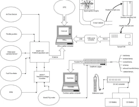
In order to measure wet concentration, the raw undiluted sample gas extracted from the exhaust system had to be maintained at about 190°C otherwise some pollutants would drop out due to condensation. Furthermore, the extracted exhaust sample must be hot filtered so that the sample cell remains free of particulates which would contaminate it and shorten its lifetime. A sample handling unit was acquired to perform these functions. The sample handling unit uses a pump to continuously extract sample from the vehicle’s exhaust system at a constant flow rate (~2L/min) via a heated line. This is then filtered using a 2 µm filter and introduced via another heated line into the sample cell of the FTIR. Both heated lines were controlled to 190°C by the sample handling unit. The sample handling unit consumes the most power since it performs heating and pumping functions. It was installed in the boot of the car along with the FTIR. The gas sample was taken downstream of the catalyst and the heated sample line was passed through a small hole in the car’s floorpan. There was no possibility of dilution of the sample by pressure pulsations from the tailpipe.

MEASURING POLLUTANTS USING FTIR

Figure 1: Block diagram of on-board system

An FTIR was chosen because of its ability to speciate hydrocarbons and NOx. With lean-burn engines, the output of NO2 increases relative to NOx, and most of the current on-board systems cannot measure NO2 and NO simultaneously. Another reason for the FTIR is the need to measure certain toxic hydrocarbons that are of interest to health-related studies.

The FTIR measuring principle is as follows: An infrared (IR) source produces a broad band IR radiation which is modulated by an interferometer. The interferometer performs an optical inverse Fourier transform. The modulated IR radiation passes through the sample cell, where sample gas absorbs certain wavelengths of the IR radiation. The detector detects the transmitted radiation and the signal is digitized. A computer then performs a mathematical Fourier transform on the digitized modulated signal and an absorbance spectrum is obtained. This spectrum is then compared to a background spectrum made initially before the measuring commenced. The Calcmet software then determines the concentrations of the components present based on absorption data from previous

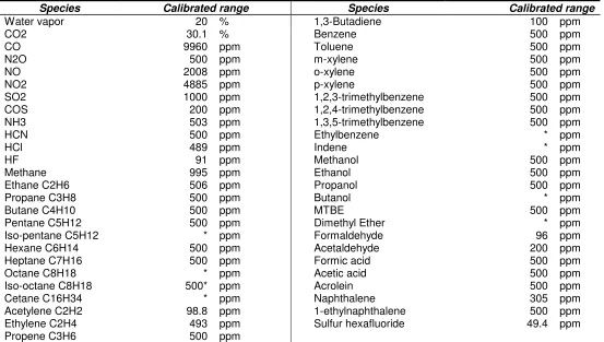
factory-performed gas calibrations. All the major species in the engine exhaust were included in the unique 51-species calibration performed by Temet for the particular instrument used in this work. A table of the measurement components and their ranges are included in the appendix. The Temet FTIR gives a warning if the calibrated compounds do not account for the observed infrared absorption in the spectra, indicating that a significant species was present that had not been calibrated for. This was not a significant problem in the present work.

signal-to-noise ratio while providing enough resolution to distinguish most compounds using the Calcmet software.

The software uses a modified CLS (Classical Least Squares) algorithm for the multi-component analysis [29]. This algorithm is adequate provided that the number of data points in the spectral region used for the analysis is twice the number of analysis components. This means that for 50 components at 8 cm-1 wavenumber resolution, a minimum 800cm-1 of spectrum is required for the analysis. This condition is satisfied as the recorded spectrum in this instrument covers 900-4250cm-1.

The detector is a liquid nitrogen cooled MCT (Mercury Cadmium Telluride) detector that scans 10 spectra per second. To enhance signal-to-noise ratio (SNR), several scans are co-added to produce a time–averaged spectrum. The SNR increases proportionally to the square root of the number of scans. Due to this averaging of spectra, the actual output interval is only 2-3 seconds. The multi-pass, gold-coated sample cell has a path length of 2m, a volume of 0.22 L and is maintained at ambient pressure and 190°C. The choice of path length and volume represents a compromise between a long path length for increased accuracy and a short path length for shorter response time. Whilst 2-3 seconds is not ideal for detailed modal emissions studies, it does provide adequate resolution for most applications. The response time will be improved in future with the shortening of the heated sample lines and the increase in the flow rate of the sample. New software will also be developed by the manufacturer in order to improve output time interval.

The Calcmet software has the additional capability of accepting analog inputs which can be logged together with the emissions spectra and analysis data. Some of these analog inputs were used to log road speed, fuel mass flow, air mass flow, throttle position, air-fuel ratio and engine speed. This then allowed the FTIR volumetric output to be converted to EI (g/kg) and g/km. The total hydrocarbons were not measured, but calculated by summing the 30 HC’s identified in the analysis.

OTHER EQUIPMENT

Fuel flow

In addition to the FTIR and the sample handling unit, in the boot of the car is a fuel flow measuring device from Max Machinery Inc. This measures the fuel mass flow rate using a level controlled recirculation tank, transfer pump and a high-resolution flow meter. The pump maintains a constant pressure to the recirculation tank which feeds fuel to the engine. This recirculation tank collects return fuel from the engine and recirculates this fuel back to the engine instead of returning it to the fuel tank. This recirculation loop allows the use of a single meter to measure make-up fuel as it replaces the fuel consumed by the engine. Total fuel consumption was determined to better than 1% accuracy and the rate of

fuel consumption was determined with a 1-second resolution. The device has an analog output which is logged on the same laptop computer used for the FTIR.

Temperatures

A DaqBook data acquisition unit was installed in the car in order to measure and log the output of the 27 K-type thermocouples attached to the various points along the exhaust and the vehicle. These outputs are recorded along with road speed on a separate laptop computer to the one being used for the FTIR. More details about the probe locations are reported by Andrews et al. [6].

Although the Temet FTIR instrument itself weighs only 21kg, the entire system as described in this paper weighs a total of ~180kg. The heaviest items are the batteries at 45kg each and the MAX fuel flow meter at 32kg. This weight is probably causing an increase in emissions as it is equivalent to carrying at least two passengers.

CALCULATIONS

Since the FTIR only measures gaseous emissions on a volumetric basis (concentration in ppm or %vol) some calculations must be performed to report the results in the requisite g/km unit. This is done by using the fuel flow rate and the air-fuel ratio. Using the equations described by Andrews et al. [6], the emission index (EI) can be calculated for each of the components under consideration. The unit of EI is (g pollutant/kg fuel). After the EI for each compound has been calculated, then the fuel flow rate is plugged into below equation giving the resulting g/s:

• Emission (g/s) = Emission EI (g/kg fuel) x Fuel flow rate (kg/hr) /3600

After calculating the emissions in g/s, the results were integrated using the trapezoidal method in order to obtain the total grams for the drive cycle. Finally, these results were divided by the drive cycle distance in order to obtain g/km for each pollutant. The instantaneous emissions could be displayed as g/kg or g/s.

VALIDATION DATA

installation in a vehicle [30]. The OBS uses hot NDIR capable of measuring CO and CO2 under wet-based conditions (sample cell kept at 120°C) by correcting interference from co-existing gases with a specially developed algorithm. This system has been validated against CVS tests and found to be within 7% for fuel consumption, 5% for CO mass emission and 6% for CO2 mass emission [30]. Exhaust flow is measured using a pitot tube attached to the tailpipe of the vehicle. THC’s are also measured using the hot NDIR, but a correction factor of 1.66 is applied since NDIR uses the absorption intensity of infrared, which is not always proportional to the number of carbon atoms in hydrocarbons. NOx and air-fuel ratio are measured using a heated ZrO2 type sensor attached on the tailpipe. Velocity and position are obtained using a GPS.

STEADY STATE VALIDATION

Steady state validation involved measuring the concentrations of various calibration bottles with CO/CH4/NO/CO2/N2 mixtures at exhaust concentration levels. Table 1 lists the results obtained from the FTIR alongside those from the MEXA-7100D and the actual certified values. The MEXA-7100D results are for an instrument calibrated on a different calibration bottle. The Temet FTIR calibration only involves zeroing the instrument using nitrogen gas. The species calibration was undertaken by Temet for 51 species and recalibration is not necessary unless any of the instrument’s hardware is changed.

Table 1: Calibration bottle #1

Certified values

MEXA-7100D

Temet FTIR

CO (ppm) 4900 4990 5324

CO2 (%) 14.50 14.00 13.86

Methane (ppm) 1509 1594 1432

NO (ppm) 1451 1403 1456

Compared to the certified values, the FTIR is within 9% for CO, 6% for CO2, 5% for methane and 0.5 % for NO. With the exception of methane, these results were deemed acceptable as they are close to the 2% of measuring range error claimed by the manufacturer. The measuring ranges are listed in the appendix. CO was within 3.3% of measuring range, CO2 within 0.5%, methane 16% and NO 2.6%. One possible reason for the excessive methane deviation is that the measurement being made exceeded the maximum methane calibration (995ppm) of the instrument.

A different bottle containing only two species was also tested and the results shown in table 2 were also acceptable, with CO being off by 0.5% and CO2 by 5.5%. In this case, CO was within 1% of measuring range and CO2 within 2.1%.

Table 2: Calibration bottle #2

Nominal values

MEXA-7100D

Temet FTIR

CO (%) 1.50 1.50 1.51

CO2 (%) 10.0 10.1 9.46

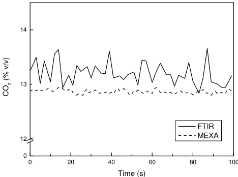
Another steady state test condition was an actual sample of exhaust gas obtained by running an engine at a steady state load of 8 kW and 2500rpm on an engine dynamometer. Figure 2 shows good agreement for CO2 except that the FTIR readings are more noisy. The MEXA results were corrected to wet because the MEXA removes water before introducing the sample to the NDIR analyzer while the FTIR samples wet exhaust. The FTIR reading is oscillating around the 13.2% mark while the MEXA is steady at 12.8%. All sampling was done immediately downstream of the catalyst.

0 20 40 60 80 100

0 12 13 14

FTIR MEXA

C

O2

(

%

v

/v

)

Time (s)

Figure 2: Steady state CO2 comparison

0 20 40 60 80 100 0

500 1000 1500 2000 2500 3000 3500

FTIR MEXA

C

O

(

p

p

m

)

Time (s)

Figure 3: Steady state CO comparison

Figure 4 shows that the NOx measured by the FTIR is higher than that measured by the MEXA. It can also be seen that the FTIR has a slower response time and cannot detect the fast changes in NOx.

0 20 40 60 80 100

0 40 50 60 70 80 90 100

FTIR MEXA

N

Ox

(

pp

m

)

Time (s)

Figure 4: Steady state NOx comparison

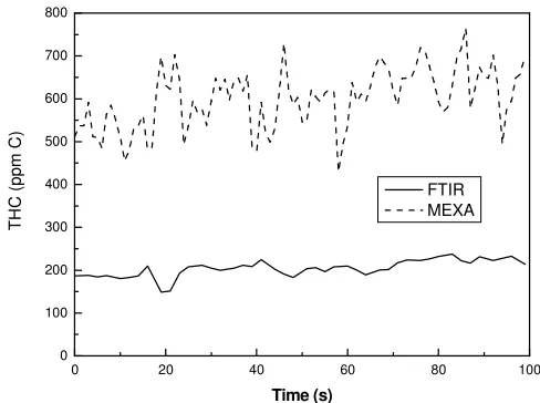
As expected, Figure 5 shows that the FTIR measured THC does not agree with the MEXA measurements. This is because the MEXA is a true total hydrocarbon analyzer and counts the number of carbon atoms using the FID technique, while the FTIR simply sums all the hydrocarbons it has identified in its analysis. This FTIR is calibrated for only 30 hydrocarbons, whereas there are typically ~160 present in exhaust gas [31]. It appears that a correction factor of approximately three needs to be applied to the FTIR readings if they are to agree with MEXA’s total HC measurements. However, this factor may vary with the level and characteristics of the THC’s and therefore no correction was applied to any data reported in the present work. The key advantage of the

FTIR is to determine individual toxic HC’s online, as will be demonstrated later.

0 20 40 60 80 100

0 100 200 300 400 500 600 700 800

FTIR MEXA

T

H

C

(

ppm

C

)

Time (s)

Figure 5: Steady state THC comparison

Table 3 summarizes the results from the steady state engine experiments and calculates the resulting error. The results reported in this table are the average readings taken over the 100 second sampling time. The error is substantial for the THC but the other components are well within the accepted limits of 20%. Possible causes of the discrepancy are the slow response time of the FTIR in addition to potential interference from other co-existing components including water. Error in the factory gas calibrations of the instrument is possible but unlikely.

Table 3: Steady state engine MEXA vs FTIR

MEXA-7100D

Temet FTIR % Error

CO (ppm) 2568 2260 -12

CO2 (%v/v) 12.8 13.2 +3

THC (ppm) 599 205 -66

NOx (ppm) 72 81 +13

TRANSIENT VALIDATION

runs using the AC dynamometer. This is to show that the repeatability of the dynamometer is excellent. The three lines in Figure 6 overlap most of the time, and that is why only one solid is visible. Consequently, this means that emissions data can be compared from different experiments as long as the initial engine conditions are the same.

0 50 100 150 200 250 300 350 400

0 1000 2000 3000 4000 5000

0 50 100 150 200 250 300 350 400

-50 -25 0 25 50 75 100 125 150

0 50 100 150 200 250 300 350 400

0 20 40 60 80 100

0 50 100 150 200 250 300 350 400

0 20 40 60 80 100 E n g in e s p e e d ( rp m )

T i m e ( s )

T o rq u e ( N m ) T h ro tt le p o s it io n ( % )

R u n 1 R u n 2 R u n 3

R o a d s p e e d ( k m /h )

Figure 6: AC dyno repeatability

Figure 7 shows the CO2 concentration from the FTIR and the MEXA overlaid. It appears reasonable to conclude that the FTIR follows the MEXA trend well but tends to slightly underestimate. The dry CO2 readings from the MEXA were corrected to wet assuming a 12% water concentration in the exhaust, which is reasonable for stoichiometric operation [32]. It must be noted that this stage of the validation was done upstream of the catalyst in order to subject the FTIR to the worst possible conditions that can be experienced on the road.

0 50 100 150 200 250 300 350 0 2 4 6 8 10 12 14 16 C O2 ( % v /v ) Time (s) FTIR MEXA

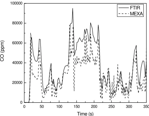
Figure 7: FTIR vs. MEXA for CO2

Figure 8 shows the CO results from the FTIR are close to the MEXA. Figures 7 and 8 show that the FTIR has a slightly lower response than the MEXA-7100D, both readings having been corrected for the sample dead time due to the sample line length (as these were different for the two instruments). There are transients which are measured by the MEXA but not by the FTIR. To study these in detail, Figure 9 enlarges a 20-second section of Figures 7, 8, 10 and 11 in order to show the differences in response time for the MEXA and the FTIR. It can be seen from Figure 9 that the MEXA will respond in as little as 1 second whereas the FTIR needs at least 2 seconds and usually up to 4 seconds in order to measure a sudden change in emissions. This causes the FTIR to miss transients that last for less than 2 seconds. Also noticeable is the longer time required by the FTIR to recover from measuring a peak. This causes the total emissions to be slightly higher than they would be when the integral is calculated.

0 50 100 150 200 250 300 350 0 20000 40000 60000 80000 100000 C O ( p p m ) Time (s) FTIR MEXA

210 212 214 216 218 220 222 224 226 228 230 0 4 8 12 16

210 212 214 216 218 220 222 224 226 228 230

0 1000 2000 3000 4000

210 212 214 216 218 220 222 224 226 228 230

0 20000 40000 60000 80000 100000

210 212 214 216 218 220 222 224 226 228 230

0 10000 20000 30000 40000 50000 C O2 ( % v /v )

T i m e (s)

N Ox ( p p m ) C O ( p p m ) T H C ( p p m ) FTIR MEXA

Figure 9: Detail of MEXA-FTIR response

Figures 10 and 11 plot NOx and THC respectively. The MEXA-measured NOx peaks are slightly higher than the FTIR readings, but this is probably a result of the FTIR’s slower response time preventing it from measuring these momentary spikes in NOx.

0 50 100 150 200 250 300 350 0 500 1000 1500 2000 2500 3000 3500 4000 N O ( p p m ) Time (s) FTIR MEXA

Figure 10: FTIR vs. MEXA for NOx

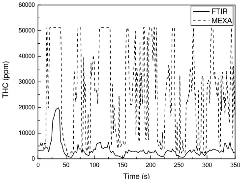
THC measured by the MEXA counts every C atom in the sample, whereas the FTIR sums all of the hydrocarbons being analyzed to derive the THC (as methane equivalent). For this reason, the FTIR reading was expected to be a gross underestimation and Figure 11 confirms this. Had more HC components been analyzed for, then the FTIR reading might have been closer to the MEXA reading.

0 50 100 150 200 250 300 350 0 10000 20000 30000 40000 50000 60000 T H C ( p p m ) Time (s) FTIR MEXA

Figure 11: FTIR vs. MEXA for THC

The results from this transient validation were not as good as for steady state validation but they were still within acceptable limits (20%) apart from THC.

REPEATABILITY

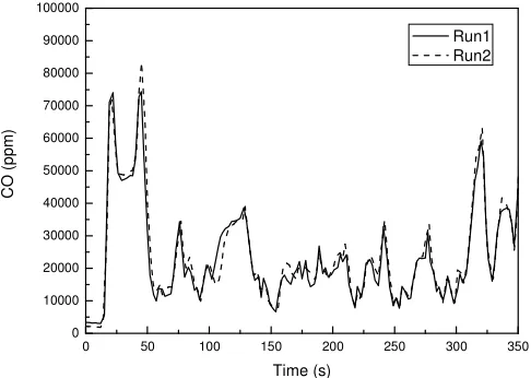
To test the repeatability of the FTIR, two separate runs were made using the AC dynamometer (which had proven to be very repeatable). These two plots were overlaid for each of the four components measured. Figure 12 shows the CO2 results and it can be seen that the repeatability is very good.

0 50 100 150 200 250 300 350 0 2 4 6 8 10 12 14 C O2 ( % v /v ) Time (s) Run1 Run2

Figure 12: FTIR CO2 repeatability

0 50 100 150 200 250 300 350 0

10000 20000 30000 40000 50000 60000 70000 80000 90000 100000

C

O

(

p

p

m

)

Time (s)

Run1 Run2

Figure 13: FTIR CO repeatability

0 50 100 150 200 250 300 350 0

5000 10000 15000 20000

T

H

C

(

p

p

m

C

)

Time (s)

Run1 Run2

Figure 14: FTIR THC repeatability

0 50 100 150 200 250 300 350 0

500 1000 1500 2000 2500

N

Ox

(

p

p

m

)

Time (s) Run1

Run2

Figure 15: FTIR NOx repeatability

ADVANTAGES OF FTIR

One of the major factors why an FTIR analyzer was chosen for use in this system was its ability to differentiate between various hydrocarbon species in a gaseous mixture. The US EPA has identified 21 mobile source air toxics, including toluene, benzene, formaldehyde, 1,3-butadiene, acetaldehyde, and diesel particulate matter, all of which can cause cancer or other serious health problems [33]. Figure 16 plots the more important hydrocarbon species that are measured by the US EPA when assessing air quality. This is simply to demonstrate that the FTIR has the potential to be a very useful instrument in any work involving toxic emissions. The drive cycle used for these graphs was a cold start Leeds LU-UDTC [6], and it must be noted that the magnitude of the results should not be considered accurate because validation of the instrument’s speciated hydrocarbon components has not been done yet. Future work will involve comparing the output of the FTIR to a standard GC-MS and a CI-MS (Chemical Ionization Mass Spectrometer).

All the hydrocarbons in Figure 16 show a dramatic drop after the first 200 seconds of the drive cycle. This is typical of a cold start. Formaldehyde seems to be less affected by the cold start than the others since it is dependent on oxygen availability, which is not present under the rich cold start conditions. After 200 seconds a combination of the catalyst lighting off and the ECU leaning the mixture to stoichiometric brings the emissions down to reasonable levels.

Another useful application of the FTIR is the speciation of nitrogen-containing compounds such as NH3, NO2, NO and N2O. This is shown in Figure 17. N2O concentration peaks at around the 180s mark because catalyst temperature at that point is just under 300°C, which is a temperature conducive to N2O production. NO and NO2 have very similar trends but the NO2 scale is approximately 2% of the NO scale. This is typical for spark ignition engines which do not produce as much NO2 as diesel engines. The ammonia peaks seem to correspond to the NOx peaks which correlate with high power situations. A rich excursion would normally result in some NH3.

OBS-1000 VS. FTIR

As a final validation, the FTIR was installed simultaneously with a commercially available on-board measuring system, the Horiba OBS-1000 [30]. Although data from various drive cycles was obtained, the only data reported in this paper will be from a cold start Leeds LU-UDTC. This drive cycle is an urban 1.5km loop described by Andrews et al. [6]. There are two right hand turns and four left hand turns in the cycle. There is also a 300-meter long steep downhill section followed immediately by a similar uphill section. This is where the highest engine loads are experienced. There are at least three first gear starts from a complete stop and sometimes more depending on the traffic conditions. Figure 18 shows the CO2, CO, NOx, THC and exhaust flow results from the OBS and FTIR plotted on the same graph. The CO2 measured with the OBS is lower in places due to the exhaust sampling point at the tailpipe entraining ambient air so that dilution takes place. This mainly occurs at idle speeds when the air mass flow is measured too high by the OBS. There also appears to be some dilution of the CO2 at idle. The THC, CO and NOx measurements are very close between the OBS and FTIR and for this reason the two lines plotted in Figure 18 appear to be one solid line.

Figure 19 plots the cumulative mass emissions for the various gases measured by the FTIR and the OBS. There is very good agreement for CO and CO2. Total THC measured by the FTIR was not expected to agree with the OBS, with the plot showing that the OBS measures higher than the FTIR by almost a factor of three. The large discrepancy in total NOx is not due to any inaccuracies in the FTIR measurements, but rather the longer sampling interval of the FTIR (2-3s) compared to the 1 second interval of the OBS. The larger time interval of the FTIR means NOx peaks are not as high as those detected by the OBS, and therefore when the instantaneous NOx emissions are numerically integrated, some accuracy is lost. This time factor did not affect total CO and CO2 as much as NOx because the fluctuations in the instantaneous mass emissions for those gases were not as high as for NOx. Once the FTIR software is modified to sample at shorter time intervals then the total NOx will be closer to the value measured by the OBS. In order to study the step throttle changes, Figure 20 zooms in on a 20-second section (210-230s) of the drive cycle. What is most noticeable is that the OBS detects the spikes in the sample whereas the FTIR tends to smooth out these spikes.

The main discrepancy between the OBS and the FTIR was the THC, as expected. This is because the FTIR simply sums all the hydrocarbons that it has identified in order to come up with a value for THC. The OBS on the other hand uses a NDIR cell to measure the infrared absorption of the THC. A correction factor of 1.66 is then applied in the OBS software in order to obtain true THC values. A similar correction factor is needed for the FTIR’s THC readings, but one was not applied in the

present work. Both THC’s are based on a hot wet sample.

Comparison of exhaust flow measurements obtained from the OBS and the FTIR were made. The OBS uses a pitot tube at the tailpipe while the FTIR setup uses an air flow sensor and a wide-band lambda sensor to calculate the exhaust flow. Figure 18 shows the two exhaust flows plotted side by side. The trend is very similar but the only major discrepancy is that the OBS measured a higher exhaust flow rate at idle. Once again the reason for this is strong engine pulsations at idle. This does not affect the total emission results because of the low magnitude of emissions at idle and the low exhaust flow at idle. It was found that to reduce this erroneous exhaust flow reading, a small extension tube should be installed after the pitot tube. Adding a small 100mm extension to the tailpipe reduced exhaust flow rate at idle from ~430 L/min to ~280 L/min as measured by the OBS on the same vehicle used in this work, under similar ambient conditions. This was not discovered until after the present work had been completed.

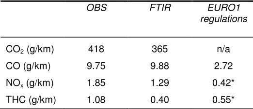
Since the exhaust flows match up well, then it is expected that the total emissions will also agree. This is shown in Table 4 where the total emissions from the OBS and the FTIR are compared for this particular LU-UDTC drive cycle. Also listed in this table are the EURO1 (1992) emissions standards for passenger vehicles. Agreement is not too good because the EURO1 drive cycle allows a 40-second warm-up period before emissions are measured and also includes the EUDC (Extra Urban Drive Cycle). Emissions for this work were measured from the moment the engine started. Furthermore, the real-world drive cycle has more transients than the legislated test cycle. Another contributing factor is probably the well-aged catalyst being used in the current study, whereas the EURO1 data is for a fresh catalyst. The OBS is higher than the FTIR for CO2 and NOx. This could be due to the overestimation of the total exhaust flow at idle, so total idle emissions are overestimated. Also the difference in time responses will contribute to higher values for the OBS. The agreement on CO was very good. Both instruments clearly show that the real-world urban drive cycle had substantially higher CO, NOx and THC emissions than the legislated drive cycle. These need to be taken into account in urban air quality modeling.

Table 4: Total emissions, FTIR vs. OBS

OBS FTIR EURO1 regulations

CO2 (g/km) 418 365 n/a

CO (g/km) 9.75 9.88 2.72

NOx (g/km) 1.85 1.29 0.42*

THC (g/km) 1.08 0.40 0.55*

*EURO1 specifies a total NOx+THC of 0.97g/km, but the EURO3

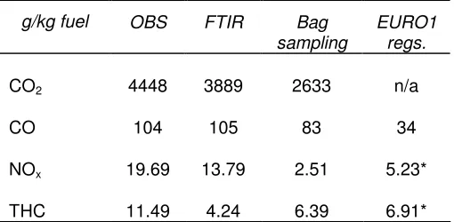
Table 5 lists the average EI results of the FTIR, OBS and bag sampling accumulated over a cold start LU-UDTC drive cycle. This bag sampling work was done by Andrews et al. [6] using the same vehicle driven over the same drive cycle. In these bag sampling tests, g/km were not reported since the fuel consumption measurement was not accurate enough to be used. There were some discrepancies in the speed-time profile since the traffic conditions during the FTIR/OBS testing were not as favourable as during the bag sampling. In addition, FTIR/OBS testing was done at 18°C ambient temperature while the bag sampling data was only available for -2°C and 32°C. The results shown in table 5 were corrected to 18°C using graphs produced by Andrews et al. [6].

Table 5: EI for FTIR vs. OBS vs. Bag sample

g/kg fuel OBS FTIR Bag sampling

EURO1 regs.

CO2 4448 3889 2633 n/a

CO 104 105 83 34

NOx 19.69 13.79 2.51 5.23*

THC 11.49 4.24 6.39 6.91*

*EURO1 specifies a total NOx+THC of 12.14g/kg, but the EURO3

HC/NOx ratio is listed for comparison

The on-board bag sampling system operates with water and higher boiling point hydrocarbons removed from the sample prior to the bag. This explains why the THC value of the bag sample is low. The bag sampling was not proportional and this will bias the sample towards low power conditions such as idle. Low power conditions produce less NOx and therefore this explains the significantly lower NOx collected in the bag. The same reasoning can be applied to CO2. On the other hand, CO and THC are more complicated since the engine would be producing higher CO and THC at idle, but the catalyst might be less efficient at idle and low power conditions due to its lower temperatures compared to high loads. Overall, the results from comparing bag sampling to the OBS and FTIR appear reasonable, and reveal the deficiencies of the bag sampling technique.

CONCLUSION

A system was developed to measure on-road emissions (CO2, CO, NOx and 30 hydrocarbon species) in-vehicle using a portable FTIR. Validation work proved that the FTIR is robust enough to be used in the harsh in-vehicle conditions. Repeatability of the FTIR was proved to be good, while accuracy was acceptable when compared to the standard analyzers. When compared to a commercial on-board system (OBS-1000) the FTIR was very close for all emissions except for THC. The FTIR is a relatively compact instrument that is considered suitable for in-vehicle real-world emissions investigation,

particularly when information on toxic hydrocarbon emissions is also required. The poor correlation between the FID and the FTIR must not be taken as poor THC performance from the FTIR. The FTIR was not intended to be a direct replacement for a FID, but rather it is an instrument that can speciate a large number of hydrocarbons. In future, the FTIR data can be further analyzed to obtain hydrocarbon speciation data for use in calculating ozone forming potentials.

ACKNOWLEDGMENTS

The authors would like to thank the UK EPSRC for a research grant, GR/M88167/01, for a JIF (Joint Infrastructure Fund) award for the LANTERN project (Leeds health, Air quality, Noise, Traffic, Emissions Research Network). We would also like to thank the EPSRC for the research grant, GR/S31136/01, for the RETEMM (REal-world Traffic Emissions Measurement and Modeling) project award in support of this work. Basil Daham would like to thank the University of Leeds for a research scholarship. Thanks must also be extended to Bob Boreham for his technical expertise during this work. The help of Prof. Joe Beebe and Antti Heikkilä is also much appreciated.

REFERENCES

1. Mayer, H., Air pollution in cities, Atmospheric Environment, Vol.33, pp.4029-4037, (1999).

2. UK DETR (Department of the Environment, Transport and the Regions), The Air Quality Strategy for England, Scotland, Wales and Northern Ireland, HM Stationery Office, (2000).

3. US EPA (Environmental Protection Agency), National air quality and emissions trends 1998. EPA-454/R-00-003, Research Triangle Park, NC 27711, (2000).

4. UK DEFRA (Department for Environment, Food & Rural Affairs), Review and assessment: Draft Technical Guidance, Report LAQM.TG(02), HM Stationery Office, (2002).

5. Peter Eastwood, Critical Topics in Exhaust Gas Aftertreatment, Research Studies Press, (2000). 6. Andrews et al, The Effect of Ambient Temperature

on Cold Start Urban Traffic Emissions for a Real World SI Car, SAE technical paper 2004-01-2903. 7. Joumard R., Jost P., Hickman J., Hassel D., Hot

passenger car emissions modelling as a function of instantaneous speed and acceleration, Science of the Total Environment, Vol. 169, pp.167-174, (1995). 8. Joumard R., Andre M., Vidon R., Tassel P., Pruvost

C., Influence of driving cycles on unit emissions from passenger cars, Atmospheric Environment, Vol. 34, pp.4621-4628,(2000).

10. B. Vogel et al., Comparison of Measured And Calculated Motorway Emission Data, Atmospheric Environment 34 (2000), pp. 2437-2450, 2000. 11. I. De Vlieger, On-Board Emission and Fuel

Consumption Measurement Campaign on Petrol-Driven Passenger Cars, Atmospheric Environment Vol.31 No.22 pp.3753-3761,1997.

12. Johannes Staehelin et al., Emission Factors From Road and Traffic From a Tunnel Study (Gubrist Tunnel, Switzrland). Part I: Concept and First Results, The Science of the Environment 169 (1995) 141-147, 1995.

13. Cory Sutela and Nick Collings, Fast Response CO2 Sensor for Automotive Exhaust Gas Analysis, SAE technical paper 1999-01-3477.

14. Cory Sutela, Nick Collings and Tim Hands, Real Time CO2 Measurement to Determine Transient Intake Gas Composition under EGR conditions, SAE technical paper 2000-01-2953.

15. Tim Hands et al., Transient SI Engine Emissions Measurement on the FTP75 Drive Cycle with a Fast Response CO Instrument, SAE technical paper 2001-01-3540.

16. Jetter J., Maeshiro S., Hatcho S. and Klebba R., Development of an On-Board Analyzer for Use on Advanced Low Emission Vehicles, SAE technical paper 2000-11-1140.

17. Timothy J.Truex et al., Measurement of Ambient Roadway and Vehicle Exhaust Emissions – An Assessment of Instrument Capability and Initial On-Road Test Results with an Advanced Low Emissions Vehicle, SAE technical paper 2000-01-1142.

18. Christopher S. Weaver and Marco V. Balam-Almanza, Development of the ‘RAVEM’ Ride-Along Vehicle Emissions Measurement System for Gaseous and Particulate Emissions, SAE technical paper 2001-01-3644.

19. Nobutaka Kihara et al., Real-Time On-Board Measurement of Mass Emission of NOx, Fuel Consumption, Road Load, and Engine Output for Diesel Vehicles, SAE technical paper 2000-11-1141. 20. Mridul Gautam et al, Measurement of In-Use, On-Board Emissions from Heavy-Duty Diesel Vehicles: Mobile Emissions Measurement System, SAE technical paper 2001-01-3643.

21. Michal Vojtisek-Lom and Joseph E. Allsop, Development of Heavy Duty Diesel Portable, On-Board Mass Exhaust Emissions Monitoring System with NOx, CO2 and Qualitative PM Capabilities, SAE technical paper 2001-01-3641.

22. http://www.cleanairt.com.

23. Nam et al., A Comparison Of Real-World and Modeled Emissions Under Conditions of Variable Driver Aggressiveness, TRB 2003 Annual Meeting. 24. Sensors, Inc, On-Road Emissions Testing of 18 Tier

1 Passenger Cars and 17 Diesel Powered Public Transportation Buses, EPA420-R-02-030, October 22, 2002.

25. Hawirko and Checkel, Real-Time, On-Road Measurement of Driving Behavior, Engine

Parameters and Exhaust Emissions, SAE technical paper, 2002-01-1714

26. Hawirko and Checkel, Quantifying Vehicle Emission Factors for Various Ambient Conditions using an On-Road, Real-Time Emissions System, SAE technical paper, 2003-01-0301

27. North et al., On-board measurements of exhaust emissions from a low-cost analyzer, Presented at Internal Combustion Engines: Performance and Emissions Conference, Institution of Mechanical Engineers, December 7-8 2004

28. J. K. Kauppinen et al., Carousel Interferometer, Applied Optics, Vol.34 No.27, pp.6081-6085, 20 Sept 1995

29. Pekka Saarinen and Jyrki Kauppinen, Multicomponent analysis of FT-IR Spectra, Applied Spectroscopy, Vol.45 No.6, pp.953-963, 1991 30. Nakamura et al., Development of a wet-based NDIR

and Its Application to On-board Emissions Measurement System, SAE technical paper 2002-01-0612.

31. Villinger et al., Dynamic monitoring of differentiated hydrocarbons in direct engine exhaust: a versatile tool in engine development, SAE Technical paper 960063.

32. Charles E. Baukal et al., John Zink Combustion Handbook, CRC Press, 2001

33. Anon, Control of Emissions of Hazardous Air pollutants from Mobile Sources, EPA Federal Register vol. 66 no.61 pp1720, March 29 2001. 34. Heeb N.V. et al., Methane, benzene and alkyl

benzene cold start emission data of gasoline-driven passenger cars representing the vehicle technology of the last two decades, Atmospheric Environment 37 (2003), pp. 5185–5195.

35. Gorse, R.A. et al., Toxic Air Pollutant Vehicle Exhaust Emissions with Reformulated Gasolines, SAE technical paper 912324.

36. Cheng W.K. et al., Auto-oil Program Phase II Heavy Hydrocarbon Study: Analysis of Engine-Out Hydrocarbon Emissions Data, SAE technical paper 941966.

CONTACT

Please direct all correspondence to Basil Daham, Energy & Resources Research Institute, University of Leeds, Leeds LS2 9JT, UK. [email protected]

ACRONYMS

LU-UDTC: Leeds Univ. Urban Drive Test Cycle HPL: Hyde Park Loop

FTIR: Fourier Transform InfraRed NDIR: Non-Dispersive InfraRed

ECE: Economic Commission for Europe FTP: Federal Test Procedure

EI: Emission index SI: Spark Ignition

CLD: ChemiLuminescence Detector ADC: Analog Digital Converter THC: Total HydroCarbons AC: Alternating Current LOD: Limit of Detection ECU: Electronic Control Unit OFP: Ozone Forming Potential CVS: Constant Volume Sampling NMHC: Non-Methane HydroCarbons VOC: Volatile Organic Compound EUDC: Extra Urban Drive Cycle

HEGO: Heated Exhaust Gas Oxygen [sensor] UEGO: Universal Exhaust Gas Oxygen [sensor] PM: Particulate Matter

APPENDIX

Table 6: FTIR measurement components and their ranges

Species Calibrated range Species Calibrated range

Water vapor 20 % 1,3-Butadiene 100 ppm

CO2 30.1 % Benzene 500 ppm

CO 9960 ppm Toluene 500 ppm

N2O 500 ppm m-xylene 500 ppm

NO 2008 ppm o-xylene 500 ppm

NO2 4885 ppm p-xylene 500 ppm

SO2 1000 ppm 1,2,3-trimethylbenzene 500 ppm

COS 200 ppm 1,2,4-trimethylbenzene 500 ppm

NH3 503 ppm 1,3,5-trimethylbenzene 500 ppm

HCN 500 ppm Ethylbenzene * ppm

HCl 489 ppm Indene * ppm

HF 91 ppm Methanol 500 ppm

Methane 995 ppm Ethanol 500 ppm

Ethane C2H6 506 ppm Propanol 500 ppm

Propane C3H8 500 ppm Butanol * ppm

Butane C4H10 500 ppm MTBE 500 ppm

Pentane C5H12 500 ppm Dimethyl Ether * ppm

Iso-pentane C5H12 * ppm Formaldehyde 96 ppm

Hexane C6H14 500 ppm Acetaldehyde 200 ppm

Heptane C7H16 500 ppm Formic acid 500 ppm

Octane C8H18 * ppm Acetic acid 500 ppm

Iso-octane C8H18 500* ppm Acrolein 500 ppm

Cetane C16H34 * ppm Naphthalene 305 ppm

Acetylene C2H2 98.8 ppm 1-ethylnaphthalene 500 ppm

Ethylene C2H4 493 ppm Sulfur hexafluoride 49.4 ppm

Propene C3H6 500 ppm

0

200

400

600

800

1000

25 50 75 100 0 25 50 75 100 0 10 20 30 0 20 40 60 80

Time (s)

20 40 60 80 100

Benzene (ppm)

1,3-Butadiene (ppm)

Acetaldehyde (ppm)

Formaldehyde (ppm)

A

/F

r

a

ti

o

Toluene (ppm)

12 14 16 18 20

S

p

e

e

d

(

k

m

/h

)

STOICH.

10 20 30 40 50

0

200

400

600

800

1000

0

20

40

60

80

100

0

5

10

15

20

0

500

1000

1500

2000

0

50

100

150

10

12

14

16

18

20

Time (s)

NH

(ppm)

NO

(ppm)

NO (ppm)

N

₂

O (ppm)

S

p

e

e

d

(

k

m

/h

)

STOICH.

10 20 30 40 50

A

/F

r

a

ti

o

0 200 400 600 800 1000 0

2000 4000 6000 0 25 50 75 100 125 150 10 12 14 16 18 20 0 10 20 30 40 50

Time (s)

FTIR

OBS

THC (ppm C)

Exhaust flow (kg/h)

A

/F

r

a

ti

o

STOICH.

S

pe

ed (

k

m

/h

)

0 200 400 600 800 1000 0

5 10 15 20 0 20000 40000 60000 0 1000 2000 3000 0 10 20 30 40 50

Time (s)

FTIR

OBS

CO

2

(%v/v)

S

p

e

e

d

(

k

m

/h

)

NO

(ppm)

CO (ppm)

0 200 400 600 800 1000 0

10 20 30 40 50 60

0 200 400 600 800 1000

0 500 1000 1500 2000 2500

0 200 400 600 800 1000

0.0 0.5 1.0 1.5 2.0 2.5 3.0 3.5 4.0 4.5 5.0 5.5 6.0

0 200 400 600 800 1000

-1 0 1 2 3 4 5 6 7 8 9 10 11

T

o

ta

l

C

O

(

g

ra

m

s

)

Time (s)

FTIR

OBS

T

o

ta

l

C

O

(

g

ra

m

s

)

Time (s)

T

o

ta

l

T

H

C

(

g

ra

m

s

)

Time (s)

T

o

ta

l

N

O

(

g

ra

m

s

)

Time (s)