Instability in the molecular dynamics step of a hybrid Monte Carlo algorithm
in dynamical fermion lattice QCD simulations
Ba´lint Joo´*and Brian Pendleton
Department of Physics and Astronomy, The University of Edinburgh, The King’s Buildings, Edinburgh EH9 3JZ, Scotland, United Kingdom
Anthony D. Kennedy
The Maxwell Institute and Department of Physics and Astronomy, The University of Edinburgh, The King’s Buildings, Edinburgh EH9 3JZ, Scotland, United Kingdom
Alan C. Irving
Theoretical Physics Division, Department of Mathematical Sciences, University of Liverpool, P.O. Box 147, Liverpool L69 3BX, United Kingdom
James C. Sexton
School of Mathematics, Trinity College, Hitachi Dublin Laboratory and Center for Supercomputing in Ireland (CSI), Dublin 2, Ireland
Stephen M. Pickles
Computer Services for Academic Research (CSAR), The University of Manchester, Oxford Road, Manchester M13 9FL, United Kingdom
Stephen P. Booth
Edinburgh Parallel Computing Centre (EPCC), The University of Edinburgh, Edinburgh EH9 3JZ, Scotland, United Kingdom 共UKQCD Collaboration兲
共Received 26 May 2000; published 17 October 2000兲
We investigate instability and reversibility within hybrid Monte Carlo simulations using a nonperturbatively improved Wilson action. We demonstrate the onset of instability as tolerance parameters and molecular dy-namics step sizes are varied. We compare these findings with theoretical expectations and present limits on simulation parameters within which a stable and reversible algorithm is obtained for physically relevant simulations. Results of optimization experiments with respect to tolerance parameters are also presented.
PACS number共s兲: 12.38.Gc, 02.70.Lq, 11.15.Ha
I. INTRODUCTION
Hybrid Monte Carlo共HMC兲 关1兴remains the most widely used algorithm for lattice QCD computations with dynamical fermions. In such computations, trial configurations are pro-duced by integrating the Hamiltonian equations of motion from an initial configuration for some fictitious molecular dynamics 共MD兲time. Configurations are then accepted or rejected by subjecting the energy change␦H along a trajec-tory to a Metropolis关2兴acceptance test.
It has been observed关3,4兴that the equations of motion in the MD evolution of such an algorithm are chaotic in the case of QCD. This implies that rounding errors induced by the use of finite precision in a digital computer may grow exponentially. Such growth can be characterized in terms of the leading Liapunov exponent of the system. Furthermore, it has been shown 关4兴that the most commonly used MD inte-gration scheme—the leapfrog method—has the potential to become unstable. Instability is a problem for lattice QCD simulations since it results in large energy changes along
MD trajectories and hence negligible acceptance rates in the HMC algorithm.
The instability in the leapfrog method has been illustrated in Ref. 关4兴for the case of free field theory where a mecha-nism has been proposed which could explain the onset of such an instability in lattice QCD. Numerical studies of the latter were carried out on small lattices at a variety of cou-plings and quark masses. The onset of instability was found to be at smaller step sizes for lighter quark masses.
Edwards, Horva´th, and Kennedy关4兴also investigated an optimization strategy in which reduced work共and hence ac-curacy兲 in the MD calculation was balanced against the re-sulting reduced acceptance in the Metropolis step. Each MD step requires the iterative solution of a system of linear equa-tions. Since dynamical fermion HMC codes spend a substan-tial fraction of their execution time performing such solu-tions, it it clearly important to investigate whether substantial efficiency gains can be made without introducing undesirable effects such as the loss of reversibility in the MD. The in-vestigation 关4兴 was quite preliminary and the errors quoted were quite large. This issue was also investigated on small lattices in Ref. 关5兴. The present paper investigates many of the issues raised in Ref. 关4兴and extends the numerical stud-ies to production-scale lattices.
*Current address: Department of Physics and Astronomy, Univer-sity of Kentucky, Lexington, KY 40506-0055.
The paper is organized as follows. In Sec. II we summa-rize the hybrid Monte Carlo algorithm and give details of the component algorithms used. Section III contains a discussion of the effects of numerical roundoff errors on reversibility. In Sec. IV we present results and discussion of our analysis of instability in the MD step. In Sec. V we present the results of an optimization analysis involving reduced accuracy in the MD step. Finally, in Sec. VI we summarize our results and conclusions.
II. HYBRID MONTE CARLO ALGORITHM AND LATTICE QCD
A. HMC algorithm
Consider a system with canonical coordinates q and ac-tion S(q). One wishes to generate configuraac-tions q with an equilibrium probability distribution in which the statistical weight of configuration q is proportional to e⫺S(q). In the hybrid Monte Carlo algorithm, we introduce fictitious mo-menta p conjugate to q and define a Hamiltonian function H(q, p)⫽p2/2⫹S(q).
One may then generate configurations (q, p) distributed according to
P共q, p兲dq d p⫽1 Z e
⫺H(q, p)dq d p
where
Z⫽
冕
dq d p e⫺H(q, p). 共1兲After the integration over the momenta, we obtain the de-sired distribution for the coordinates. Given an initial con-figuration (q, p), a sequence of concon-figurations is generated by repeated iteration of the following steps.
共1兲Momentum refreshment. Draw new fictitious momenta p from a Gaussian distribution with zero mean and unit vari-ance.
共2兲Molecular dynamics. Integrate the Hamiltonian equa-tions of motion for some fictitious time trajectory of length, from the initial configuration„q(0), p(0)…⫽(q, p) to obtain the trial configuration „q(), p()…⫽(q
⬘
, p⬘
).共3兲 Accept/reject step. The trial configuration (q
⬘
, p⬘
) is accepted with probabilityPacc共q
⬘
, p⬘
←q, p兲⫽min共1,e⫺␦H兲, 共2兲where
␦H⫽H共q
⬘
, p⬘
兲⫺H共q, p兲. 共3兲If the trial configuration is rejected the new configuration is (q, p).
B. Leap-frog integration
For the HMC algorithm to satisfy detailed balance, the MD is required to be reversible and measure preserving. This can be achieved through the use of symmetric symplectic integration schemes, such as the leapfrog algorithm. In this
algorithm, one constructs an approximation U3(␦) to the time evolution operator U(␦) for advancing a phase space vector (q, p) through a step of length ␦ in molecular dy-namics time. The approximate operatorU3(␦) is itself com-posed of a symmetric combination of the symplectic partial coordinate and momentum update operators Uq(␦) and
Up(␦), respectively, for example as
U3共␦兲⫽Up
冉
␦2
冊
Uq共␦兲Up冉
␦2
冊
. 共4兲The partial update operators are themselves defined as
Uq共␦兲共q, p兲⫽共q⫹p␦, p兲, 共5兲
Up共␦兲共q, p兲⫽共q, p⫹F␦兲, 共6兲
where F⫽⫺S/q is the MD force. Because of its symmet-ric construction, U3(␦) is reversible and, due to the sym-plectic nature of its component updates, it is area preserving. The process of iteratively acting on an initial phase space vector with U3(␦) is called leapfrog integration. The method is accurate to O(␦3) per time step.
C. Higher order integration schemes
The construction of higher order integration schemes共see, for example, Refs. 关6,7兴兲 is recursive, proceeding from the leapfrog scheme. Given an approximate time evolution op-erator Un⫹1(␦) accurate to O(␦n⫹1) for some even n, one can construct the operator
Un⫹3共␦兲⫽Un⫹1共␦1兲iUn⫹1共␦2兲Un⫹1共␦1兲i 共7兲
with
␦1⫽ ␦
2i⫺s, 共8兲
␦2⫽ ␦
1⫺共2i兲/s, 共9兲
where i is an arbitrary positive integer and s⫽(2i)1/(n⫹2). The step sizes ␦1 and␦2 are chosen to cancel truncation errors of O(␦n⫹1) and symmetry with respect to time en-sures that there are no truncation errors of O(␦n⫹2). Hence such a scheme is accurate to O(␦n⫹3).
D. Formulation of MD for lattice QCD
The canonical coordinate variables for lattice QCD are the SU共3兲link matrices U(x) associated with the link emanat-ing from site x of the lattice and endemanat-ing on neighboremanat-ing site x⫹ˆ , where ˆ is a unit vector in one of the Euclidean space-time directions. The conjugate momentum fields (x) are members of the Lie algebra su共3兲.
In general, one can write the fictitious Hamiltonian for a lattice QCD system with two degenerate flavors of Sheikholeslami-Wohlert 共clover兲 improved 关9,10兴 fermions as
H˜⫽1 2
兺
x, 2⫹
Sg共;U兲⫹†Q˜⫺1共,c;U兲, 共10兲
where
Q
˜共,c;U兲⫽M†共,c;U兲M共,c;U兲. 共11兲
Here M (,c;U) is the clover improved fermion matrix with improvement coefficient c, are pseudofermions and Sg(;U) is the standard Wilson gauge action
Sg共;U兲⫽⫺
6
兺
䊐 Re Tr U䊐. 共12兲 In Eq.共12兲the sum is over all elementary plaquettes U䊐 on the lattice and⫽6/g2, where g is the bare gauge coupling constant.In our computations we have employed the technique of even-odd preconditioning which changes the form of Q˜ and H˜ somewhat. Each lattice site is labeled with a parity p which is either even or odd so that any one lattice site has an opposite parity from all of its neighbors. This allows the fermion matrix to be block diagonalised and the Hamiltonian to be rewritten as
H⫽1 2
兺
x, 2⫹Sg共;U兲⫺2 Tr ln A
e⫹o
†
Q⫺1共,c;U兲o.
共13兲
Here, A is the so called clover term summed over sites of one parity 共even in the equation above兲 and Q is the precondi-tioned fermion matrix coupling lattice sites of the opposite parity共odd in the equation above兲only. Thus Q has half the rank of Q˜ . This leads to some memory saving at the addi-tional expense of having to evaluate Tr ln A directly on sites of one parity. The precise formulation of the preconditioned matrices can be found in Ref. 关11兴.
We do not expect that splitting the Hamiltonian in this way will change conclusions regarding reversibility and re-lated issues in any significant way. Although there is an extra force term to be computed to integrate the equations of mo-tion, the logarithm of the clover term is computed directly and is independent of the parameters used for the solution of the system of linear equations. Likewise, for the inversion of the clover term, we use a direct method that is not controlled by algorithmic parameters such as a target relative residue.
Hence we regard the effects of preconditioning as a minor technicality and shall disregard them for the rest of this pa-per.
The leapfrog partial update steps for the gauge fields and the momenta are
Uq共␦兲关U共x兲,共x兲兴⫽关exp兵i␦ 共x兲其U共x兲,共x兲兴
共14兲
Up共␦兲关U共x兲,共x兲兴⫽关U共x兲,共x兲⫹␦F共x兲兴,
共15兲 where
F共x兲⫽Fg共x兲⫹Ff共x兲 共16兲
and Fg, Ffare the respective gauge and fermionic force con-tributions
Fg共x兲⫽⫺Sg共U兲
U共x兲, 共17兲
Ff共x兲⫽关Q⫺1兴† Q U共x兲 关Q
⫺1兴. 共18兲
E. Solution of the linear system
Computation of the fermion force requires the quantity
X⫽Q⫺1 共19兲
which is obtained via the solution of the linear system
QX⫽. 共20兲
This is normally carried out with a Krylov subspace solver such as the conjugate gradients 共CG兲 关12兴 or the stabilized biconjugate gradients 共BiCGStab兲 关13兴 algorithm. With the BiCGStab solver, the solution consists of two solves:
M†共,c兲Y⫽, 共21兲
M共,c兲X⫽Y , 共22兲
whereas with CG, one can solve Eq. 共20兲 directly. When using CG with a Hermitean positive definite matrix such as Q, the solution is guaranteed to converge monotonically. With BiCGStab, one has no such guarantee. Since the con-dition number of Q is the square of the concon-dition numbers of either M or M†, we expect the two stage solution using BiCGStab to be faster on the whole than using one CG solve. As the convergence of BiCGStab can be erratic, it is prudent to restart the solution process for X with CG using, as an initial guess, the solution for X from the previous BiCGStab solve.
The solver residual ri at the ith iteration of a CG solve is defined as
rireal⫽储⫺QXi储, 共23兲
where Xi is the approximate solution at iteration i. The
i
real⫽ri real
储储. 共24兲
In solver algorithms, riis not usually computed using Eq.
共23兲. Instead, riis generally defined through some three term
or coupled two term recurrence relation. We will refer to this latter definition of the residual as racc, the accumulated re-sidual. The corresponding definition of the relative residual is
i
acc⫽ri
acc
储储. 共25兲
These two definitions are equivalent in exact arithmetic. However, computation of the accumulated residual needs only vector additions and scalar multiplications whereas computation of the real residual needs a matrix multiplica-tion and so the two can differ in finite arithmetic. In our computations we use the accumulated residual. We will de-note by r our target relative residual. Hence the iterative process terminates when iacc⬍r. In the remainder of this paper we refer to r as the solver target residual, or just sim-ply the solver residual.
III. REVERSIBILITY
Reversibility and area preservation of the Molecular Dy-namics step are required for a correct HMC algorithm. The leapfrog algorithm described in Sec. II, is reversible and area preserving in exact arithmetic. Computations are of necessity carried out in finite precision and exact reversibility is lost. It is therefore important to verify that implementation of the fundamental steps of the algorithm are as close to reversible as it is possible to make them.
Ideally, one would like to establish the least level of pre-cision required such that the accumulation of rounding errors does not introduce a significant bias into the end results of a calculation. At present, it is not possible to give a fully quan-titative answer to this question. The accumulation of round-ing errors is a complex phenomenon and, since the underly-ing equations of motion are known to be chaotic, the potential for introducing large uncontrolled errors is great 关3,4兴. The best one can do is to ensure that the implementa-tion of each algorithmic component is as close to reversible as practical and that the accumulation of errors grow in the expected way and so remain under control. We study the reversibility of gauge and momentum update components separately.
A. Gauge update
The gauge update involves the process of exponentiating the conjugate momenta on all lattice links 关14,15兴. One wishes to verify here that the exponentiation of the momenta does produces a suitable unitary matrix, and the exponentia-tion of the momenta is reversible in the sense that
exp关i共x兲␦兴⫽exp关⫺i共x兲␦兴†. 共26兲
To check these properties, we studied
⌬unit⫽ max
x,,a,b兩兵exp关i共x兲␦兴exp关i共x兲␦兴 †⫺1其
ab兩
共27兲 ⌬rev⫽ max
x,,a,b兩兵exp关i共x兲␦兴⫺exp关⫺i共x兲␦兴 †其
ab兩,
共28兲
where x, , a, and b are site, direction, and color indices, respectively. These observables measure the maximum vio-lations of unitarity and hermiticity on a given lattice.
In tests of the gauge field update reversibility, we used quenched lattices with V⫽44 sites at ⫽5.4. For the MD evolution we used ⫽1 and ␦⫽ 1
10. The maximum values
of both ⌬unit and ⌬rev along a molecular dynamics trajec-tory were found to be
max
traj ⌬unit⫽maxtraj ⌬rev⫽0.59604635⫻10
⫺7⬇1 2⑀SP,
共29兲
where⑀SPis the single precision unit of least precision. The fact that the maxima of the metrics agree to eight decimal places may seem surprising at first, but becomes less myste-rious when we recall that we are working at the limits of single precision, where the discrete nature of floating point numbers on a computer becomes apparent. Hence, there is only a discrete set of values available that the metrics can take of which the figure quoted above is one.
B. Momentum update
In the momentum update there are two possible sources of reversibility violation. The first is a lack of associativity in the addition p(⫹␦)⫽p()⫹F(U)␦ required in the up-date step. The second arises in the computation of the force F. However, when performing a momentum update forward in time for a step ␦ followed immediately by a momentum step backwards in time for␦ 共with no gauge field update in between兲 the gauge fields, and hence the force, should re-main unchanged. Thus, reversibility due to lack of associa-tivity in the addition can be isolated.
Consider a test where one starts with a set of fields (U,,). First the momentum fields are updated forward in time for a timestep␦ to produce fields (U,
⬘
,) and then a momentum update is performed backwards in time1to pro-duce fields (U,⬙
,). We use the same value of the force F for both of the updates. One can then define the quantity⌬i共x兲⫽i共x兲
⬙⫺
i共x兲 共30兲as a measure of the reversibility violation incurred by the momentum update step. To improve statistics, one may re-peat this several times, in each case using a new set of initial momenta drawn from a Gaussian distribution.
In the numerical tests, we started from some initial gauge field configuration and performed MD in the ordinary sense. Before every momentum update, we performed 100
forward-1In practice this is done by flipping the signs of all the momenta,
backward steps with newly drawn momenta in each case. After the test was completed, we restored the original mo-menta from the end of the last gauge update step and allowed the MD to continue. Thus we obtained an estimate of
具
⌬i(x)典
, the average reversibility violation due to lack ofassociativity in the addition. At the end of the complete tra-jectory, the resulting data was split into eight sets, one cor-responding to each of the Lie algebra indices i. The data in each set was histogrammed to obtain the distribution of the average reversibility violation for each momentum compo-nent.
[image:5.612.53.296.56.274.2]The results of these momentum update tests are shown in Fig. 1. We show the histograms of all eight momentum com-ponents. The errors on the data points are small and, to aid clarity, are not displayed. The lattice volume used for these tests was V⫽43⫻8 sites and physical parameters were  ⫽5.2, c⫽0 and⫽0.1360. We performed the tests follow-ing each gauge field update along a trajectory consistfollow-ing of 10 timesteps, each of length␦⫽0.1. We used 500 bins for each momentum component in the histograms. The histo-gramming process itself was carried out in double precision, allowing us to resolve reversibility violations of O(10⫺1⑀SP).
Figure 1 shows that the distribution of reversibility viola-tions forms a very narrow, apparently symmetric, distribu-tion around 0 with a width that is of O(10⫺1⑀SP). We con-clude that the momentum update step in itself is as reversible as it is possible to attain. The apparent symmetry of the distribution may possibly be used to make more general statements about reversibility and area preservation holding stochastically 关16兴.
C. Reversibility of the force computation
Since gauge fields are unchanged along a momentum up-date and computation of the force due to gauge fields is an
entirely deterministic process, one expects that the force computation will be reversible. However, the pseudofermion contribution to the force requires the solution of linear equa-tions, so further scrutiny is required.
It has been pointed out 关17兴 that the solution process should be reversible, provided that a time symmetric initial guess vector共such as a zero vector or a vector with random components兲is used to start the solution process. This makes it tempting to carry out such solves with a large target resi-due r, and hence save on the computational workload. We discuss this further in Secs. III G and V.
Another commonly used solver strategy is to use the so-lution from the force computation of the previous momen-tum update as an initial guess. This, and variants which use a more elaborate extrapolation of previous solutions, may re-duce the computational workload but are inherently non-reversible unless the solutions are effectively exact.
D. Global reversibility violations
Having discussed the sources of reversibility violation at a microscopic level, we now turn to the problem of their global accumulation. Consider an MD trajectory with initial fields (U,) and a set of pseudofermion fields. The latter remain unchanged along an MD trajectory. Suppose we perform an MD trajectory forward to obtain fields (U
⬘
,⬘
), then having reversed the momenta, perform a second 共backward兲 trajec-tory and a momentum flip to obtain fields (U⬙
,⬙
). One may define the following global reversibility violation metrics:储⌬␦U储⫽
冑
兺
x,,a,b 兩
Uab共x兲
⬙⫺
Uab共x兲兩2, 共31兲储⌬␦储⫽
冑
兺
x,,i 关
i共
x兲
⬙⫺
i共x兲兴2, 共32兲兩⌬␦H兩⫽兩H共U
⬙
,⬙
,兲⫺H共U,,兲兩. 共33兲It is also useful to consider these quantities suitably normal-ized by their respective degrees of freedom
储⌬␦U储d.o.f⫽储⌬␦U储
冑
Nd.o.fU , 储⌬␦储d.o.f⫽ 储⌬␦储冑
Nd.o.f , and兩⌬␦H兩d.o.f⫽ 兩⌬␦H兩
冑
Nd.o.fH . 共34兲Here Nd.o.fU ⫽Nd.o.f ⫽4⫻8⫻V are the respective number of the gauge and momentum degrees of freedom 关4 links per site and 8 SU共3兲 generators兴and Nd.o.fH is the number of de-grees of freedom involved in computing the Hamiltonian H. In the quenched approximation Nd.o.fH ⫽Nd.o.fU ⫹Nd.o.f . When dynamical fermions are included, there is an additional factor from the fermions of Nd.o.ff ⫽24⫻V 共three color and four Di-rac complex components per site兲. In the even–odd precon-ditioned systems, half of the Nd.o.ff degrees of freedom are FIG. 1. Distribution of momentum update reversibility
viola-tions obtained by histogramming具⌬典. Each plot corresponds to a separate momentum component and⑀SPis the single precision unit
represented in the pseudofermion vectors and the remainder absorbed into computing Tr lnA on sites of the opposite parity.
We also study兩⌬␦H兩/兩␦H兩, where
␦H⫽H共U
⬘
,⬘
兲⫺H共U,兲. 共35兲This is a measure of the relative error in our energy calcula-tions and is related to the accuracy of the acceptance prob-ability. One would like this relative error to be quite small, certainly no more than a few percent.
E. Volume scaling of global reversibility metrics
According to their definitions,储⌬␦U储 and储⌬␦储 should scale as O(
冑
V), since the metrics require the summation of O(V) positive definite quantities. We therefore expect that the corresponding normalized 共per degree of freedom兲 met-rics should volume independent. For兩⌬␦H兩, the summation involves numbers which are not positive-definite, and one might expect some cancellation. If the numbers are truly ran-dom, the cancellations between the terms can be modelled as a random walk and one would expect the sum to scale as O(冑
V). Hence one would expect 兩⌬␦H兩d.o.f to be indepen-dent of the system volume in a manner similar to the 储⌬␦U储d.o.fand储⌬␦储 metrics.To satisfy ourselves further that our simulation code is performing as well as can be expected, we carried out re-versed trajectories共as described in the definition of the met-rics兲in the quenched approximation with lattices of different volumes. In each case, we used a single configuration as the starting gauge field for the test and the momentum field was drawn randomly from a heat bath. The trajectory length was
⫽1 and the length of the timestep was␦⫽ 1
180. We used
⫽5.4 and lattices of volume
V苸兵44,84,103⫻16,163⫻32其. 共36兲
Results of these tests are shown in Fig. 2 where the vol-umes have been normalized by the smallest one (V0⫽44). We note that the degree of freedom normalized metrics– 储⌬␦U储d.o.f, 储⌬␦储d.o.f, and 储⌬␦H储d.o.f–are all independent of the volume as expected. We also note that the relative error 兩⌬␦H兩/兩␦H兩 is less than of order 0.1%, showing that error in computing the acceptance probability is small.
F. Accumulation of rounding errors in MD time
It has been noted by several authors that the MD equa-tions of motion are chaotic 关3,4兴and so effects of roundoff error are expected to grow exponentially with MD time along a trajectory. In particular, if one were to carry out reversed trajectory tests, as described in the definition of the metrics 储⌬␦U储 and储⌬␦储, these would be expected to ex-hibit the leading behavior
储⌬␦U储⬀eU and 储⌬␦储⬀e 共37兲
as a function of the MD trajectory length. We use this as an operational definition of the effective leading Liapunov ex-ponentsUand. In our computations we measured only
U and, hence, in future discussion we shall drop the
sub-script U and refer to it simply as. We shall also refer to simply as the Liapunov exponent.
[image:6.612.51.424.56.332.2]The authors of Refs. 关3–5兴 all found positive values for the Liapunov exponents in their studies. In particular it was shown in Ref. 关4兴that as the solver target residue r and MD FIG. 2. Volume scaling of re-versibility metrics, 储⌬␦U储d.o.f,
储⌬␦储d.o.f, 兩⌬␦H兩d.o.f, and
兩⌬␦H兩/兩␦H兩. The volumes are normalized by the smallest vol-ume used: V0⫽4
4
step-size␦ were made smaller, the Liapunov exponents ap-peared to plateau, indicating that chaos was present in the underlying continuum equations of motion for the system and not just a feature of the numerical integration scheme.
For the leading Liapunov exponent, the authors of Ref. 关4兴found that this plateau came to an end at␦⬇0.6 in the quenched approximation and in the case of dynamical fer-mion simulations with sufficiently heavy quarks. Beyond this step size, the effective exponent exhibited growth. However, in the case of light quarks, this growth was found to set in significantly earlier, at␦⬇0.08. This sudden growth in Lia-punov exponents could signal the onset of instability in the MD. The subject of integrator instabilities will be taken up in Sec. IV.
The authors of Ref. 关4兴 also studied the behavior of the Liapunov exponents as a function of the MD solver target residue r. They investigated the effects of increasing r共using a time symmetric start兲 as a possible means of improving computational efficiency. Their data indicated a sudden growth in Liapunov exponent as r is increased beyond a critical value. The data covered a limited range of r, and had large statistical errors. However, the sudden apparent growth of the Liapunov exponent coincides with a dramatic drop in acceptance rate, suggesting again that the integrator has be-come unstable.
G. Tuning the solver target residual
The results of Ref.关4兴motivated us to measure the Lia-punov exponents of our simulations while varying the target residue of a comparatively large volume system, with com-paratively light quarks such as those in current production runs. For the determination of Liapunov exponents, we used 10 configurations taken from one of our large data sets. The lattice volume used was V⫽163⫻32 and the physical param-eters were⫽5.2, c⫽2.0171, and⫽0.1355. The value of the clover coefficient was calculated using the formula
deter-mined by the Alpha Collaboration 关10兴. These parameters correspond to pseudoscalar to vector mass ratio of m/m ⬇0.6关18兴 and a lattice spacing of a⫽0.097 fm关18兴where the physical lattice spacing has been determined using the observable r0 关19兴. By current standards, the dynamical fer-mions are relatively light.
Using the 10 starting configurations, for a given value of r we carried out reversed MD trajectories of varying length with a constant step-size of ␦⫽ 1
180. This value for ␦ was
the one used in the production of the dataset from which our ten sample configurations were taken. Our MD solver strat-egy was to employ a two stage BiCGStab solution to com-pute the quantity X of Eq. 共19兲followed by a restarted CG solution. Hence the target residue used was the accumulated target residue for the CG solver as described in Sec. II E. The target residues used ranged from r⫽10⫺7 to r⫽10⫺4. The smallest of these is near the limit of what may be achieved in a single precision 共32bit兲computation.
In each test we measured储⌬␦U储,兩␦H兩and Niters, where Niterswas the total number of solver iterations carried out in both the BiCGStab and CG solves averaged over the forward and reverse trajectories. For each combination of parameters, we also calculated the Metropolis acceptance probability Pacc.
To evaluate the savings 共or losses兲in computational cost we defined the cost metric
cost⫽Niters Pacc
. 共38兲
[image:7.612.49.353.54.306.2]This heuristic measure reflects the fact that a large number of iterations along an MD trajectory implies high computational cost, as does a low Metropolis acceptance rate. We note that an absolute measure of cost should also take into account the autocorrelation time of the ensemble produced by an HMC computation. Since we are unable to control or measure this
quantity on a sample of ten configurations, we disregard au-tocorrelation effects in this study where we are interested in the relative cost with different choices of simulation param-eters.
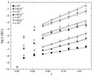
Figure 3 shows fits used to extract the 共effective兲 Lia-punov exponents. The system is clearly chaotic as ln储⌬␦U储 has a significant positive slope as a function of. Even with only ten configurations, the signal for the Liapunov expo-nents is good except for the cases when r⫽5⫻10⫺6 and when r⫽10⫺5. The data for these latter parameter values seem to show a marked break at ⬇0.6 and indeed, it was not possible to establish a consistent value of the Liapunov exponent for these two values of r.
In Fig. 4 we show
具
␦H典
, the energy change along an MDtrajectory averaged over ten configurations as a function of trajectory length . One can clearly distinguish three differ-ent types of behavior for
具
␦H典
depending on the target MD residual r. For values of r⬍5⫻10⫺6,具
␦H典
shows an oscil-latory behavior with , whereas for r⬎10⫺5具
␦H典
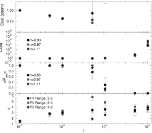
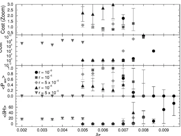
diverges with increasing , resulting in a corresponding exponential drop in acceptance probability. It is interesting to note that this change in the behavior of ␦H occurs at the value of r where the data in Fig. 3 also show a change. [image:8.612.54.353.475.736.2]A summary of results for tuning the solver residue is shown in Fig. 5. The bottom panel shows the Liapunov ex-ponents. For each value of r we made several determina-tions of by fitting to different ranges of in Fig. 3. We note that the results of these different fits are consistent with FIG. 4. 具␦H典as a function of␦ for various values of r.
each other except for the values of r⫽5⫻10⫺6 and r ⫽10⫺5 corresponding to the ‘‘break’’ evident in Fig. 3.
We note that, overall, the Liapunov exponents appear to show a slow growth with r. There is no evidence of a plateau as r is reduced to r⫽10⫺7. This implies that this manifesta-tion of chaos in the system is not due to the underlying equations of motion, but to the integrator. The behavior of the exponents near r⫽10⫺5 may perhaps be interpreted as the effect of the integrator changing from being stable to being unstable.
The second panel in Fig. 5 shows the average acceptance rate
具
Pacc典
for trajectories of length ⬇1. The acceptance shows a rapid drop for r⬎10⫺5, which is due to the diver-gent behavior of␦H for values of r in this region. The rapid drop in acceptance rate results in a huge growth in the cost of the algorithm as shown in the third panel of Fig. 5 where we display the cost metric 共38兲 normalized by its value for the simulation with r⫽10⫺7.In the top panel of Fig. 5 we show an enlarged view of the cost function for values of r⬍10⫺5. The cost metrics for values of r⭓10⫺5are too large to fit onto this enlarged plot. We note that the normalized cost has a shallow minimum when r⫽5⫻10⫺6, however, at this minimum value the nor-malized cost has a value of about 0.75 implying a saving of only about 25%.
IV. INSTABILITY IN THE MD INTEGRATION
The behavior of the energy change ␦H, from oscillatory to divergent, is reminiscent of a known instability in the leapfrog algorithm when applied to the integration of the equations of motion for the simple harmonic oscillator. In this section, we review the simple harmonic oscillator analy-sis of Ref.关4兴and compare expectations for interacting theo-ries with our numerical results.
A. Harmonic oscillator
In what follows we use the notation of Ref.关4兴. Consider a single oscillator with coordinate . The corresponding Hamiltonian function is
H⫽1 2共
2⫹22兲, 共39兲
where is the angular frequency of the oscillator and is the corresponding fictitious momentum.
The leapfrog update for the coordinate and momentum may be written in the form of a matrixU3(␦) acting on the phase space vector (,)
U3共␦兲⫽
冉
1⫺1 2
2␦2 ␦
⫺2␦⫹1 4
4␦3 1⫺1 2
2␦2
冊
. 共40兲The update matrix U3 can be parameterized as
U3共␦兲⫽
冉
cos关共␦兲␦兴sin关共␦兲␦兴 共␦兲 ⫺共␦兲sin关共␦兲␦兴 cos关共␦兲␦兴
冊
,
共41兲
where
共␦兲⫽cos⫺
1关1⫺共1/2兲2␦2兴
␦ , 共42兲
共␦兲⫽
冑
1⫺共1/4兲2␦2. 共43兲Evolution over a whole trajectory of length is then given by
U3共兲⫽
冉
cos关共␦兲兴sin关共␦兲兴 共␦兲 ⫺共␦兲sin关共␦兲兴 cos关共␦兲兴
冊
. 共44兲
The nature of the instability in the leapfrog scheme may be illustrated by examining the phase space trajectories in this system. The initial phase space vector for an oscillator released from amplitude A is 关(0),(0)兴⫽(A,0). From Eq. 共44兲, the phase space vector at time is then given by
冉
共兲 共兲冊
⫽冉
Acos关共␦兲兴
⫺A共␦兲sin关共␦兲兴
冊
. 共45兲The phase space orbits therefore satisfy
2共兲 A2 ⫹
2共兲
A22共␦兲⫽1. 共46兲
It can then be seen from Eqs. 共43兲 and 共46兲 that for ␦⬍2 the phase space trajectories are elliptical,2 whereas for␦⬎2 they are hyperbolic. The instability at␦⫽2 is the abrupt transition from one class of phase space trajecto-ries to another.
The change in energy
␦H⫽H关共兲,共兲兴⫺H关共0兲,共0兲兴 共47兲
may also be computed. Using the same initial conditions
␦H⫽⫺1 8
4A2␦2sin2关共␦兲兴. 共48兲
When␦⬍2, (␦) is real and so␦H oscillates with in-creasing, in a manner similar to that observed in the bottom panel of Fig. 4. However, when ␦⬎2, (␦) becomes purely imaginary causing␦H to diverge as sinh2关(␦)兴in a manner similar to that seen in the top panel of Fig. 4.
2In the exact solution the orbits are circular, the deformation to an
B. Generalized treatment of instabilities
We now present a more general method of finding insta-bilities in the leapfrog algorithm and in higher order schemes of the type discussed in Refs. 关6,7兴 共see Sec. II C兲 when applied to the case of a harmonic oscillator.
Consider an initial phase space vector (,) of the har-monic oscillator. This is to be evolved through phase space by the leapfrog matrix U3(␦) of Eq.共40兲. The area preser-vation property of the integrator implies that det关U3(␦)兴 ⫽1. All components ofU3(␦) are real, implying that TrU3 is also real.
If
1⫽u1⫹iv1 and 2⫽u2⫹iv2 共49兲
are the two eigenvalues of U3(␦), the previous conditions on the trace and the determinant共area preservation兲can then be shown to imply that
v1⫽⫺v2 and u1v2⫹u2v1⫽0. 共50兲
We conclude that either,共1兲u1⫽u2 or,共2兲v1⫽v2⫽0. In case共1兲, the determinant condition (12⫽1) implies that u12⫹v1
2⫽1. The eigenvalues have magnitude unity: 1,2⫽e⫾
i with real, and the update matricesU
3(␦) and
U3() 关⫽U3
NMD
(␦)兴 give stable elliptical trajectories in phase space.
In case共2兲, by the same condition on the determinant, we have that1⫽and2⫽1/ for some real⭓1. On raising 1or2 to the power NMD, one of the eigenvalues ofU3() will show an exponential divergence with NMD. This implies unstable behavior in the integrator.
The condition for the onset of instability is that the eigen-values change from being complex to real. This information can be deduced from the discriminant of the characteristic polynomial of the update matrixU3(␦). The onset of insta-bility occurs as the discriminant changes sign from negative to positive.
For the leapfrog method, the discriminant is given by
D3⫽共␦兲2共␦⫺2兲共␦⫹2兲. 共51兲
We note that for 0⬍␦⬍2, the discriminant is negative indicating a stable integrator, whereas for ␦⬎2 the dis-criminant is positive implying an unstable integrator in line with the previous discussion.
C. Instability in higher order schemes
Consider the fifth order scheme of Campostrini and Rossi 关6兴. This can be constructed from three leapfrog integration steps as
U5共␦兲⫽U3共␦1兲U3共␦2兲U3共␦1兲 共52兲
with ␦1⫽␦/(2⫺21/3) and ␦2⫽⫺21/3␦/(2⫺21/3). This corresponds to n⫽3 and i⫽1 in Eqs.共8兲and共9兲.
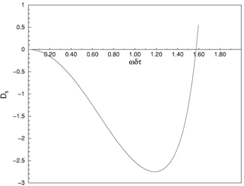
The discriminant D5is a twelfth order polynomial in␦ which can easily be found using an algebraic package such
as Maple. It is not reproduced here but plotted in Fig. 6. The nonnegative roots of the D5⫽0 are found to be
␦苸兵0,
冑
12⫺6冑
3 4其. 共53兲 To three decimal places, the positive root is at 1.573. The discriminant is negative for 0⬍␦⬍1.573 indicating stable behavior and is positive for␦⬎1.573 for the region where the integrator is unstable.It is interesting to note that, for the central leapfrog update matrixU3(␦2) in the fifth order scheme to become unstable on its own, requires that ␦2⫽2. This implies that this central step should go unstable when
␦⫽2共2⫺2 1/3兲
21/3 ⬇1.175. 共54兲
This suggests that, although the central update itself becomes unstable at ␦⫽1.175, the other two updates in the scheme stabilize the system until ␦⬇1.57.
Following a similar calculation, it can be shown that the discriminant D7 of the characteristic polynomial for the up-date matrix of the seventh order scheme (n⫽5, i⫽1) has roots at
␦苸兵0,1.595,1.822,1.869其 共55兲
with D7 being negative in the intervals D7苸(0,1.595) and D7苸(1.822,1.869) indicating two domains of stability. The discriminant is positive for D7苸(1.592,1.822) and for D7 ⬎1.869. For the longest constituent fifth order update to go unstable in this scheme requires that␦⬎1.166.
[image:10.612.317.560.56.241.2]Hence we see that, for the case of the simple harmonic oscillator at least, higher order integration schemes do not help cure the problem of instabilities. Indeed, they become unstable at even smaller values of ␦ than the simplest leapfrog method.
FIG. 6. The discriminant D5of characteristic polynomial of the
D. Hypothesis for interacting field theories
Edwards, Horva´th, and Kennedy关4兴advanced the hypoth-esis that, since the high frequency modes of an asymptoti-cally free field theory can be considered as a collection of weakly coupled oscillator modes, the instability just de-scribed in the harmonic oscillator system will also be present for interacting field theories. The onset of the instability will be caused by the mode with highest frequencymax, when max␦⫽2. For a single oscillator mode, the onset of insta-bility is abrupt. In the case of an interacting theory, one would expect the effects of the interactions to smooth out this transition.
It is argued in Ref.关4兴that the instability in lattice QCD with dynamical fermions can be likened to that of a collec-tion of oscillator modes of the sort just described. When applying leapfrog integration to this system, the role of2 in the harmonic oscillator example is played by the MD force F(x). This force can be written as a sum of contribu-tions from the gauge and fermionic pieces of the action as F(x)⫽Fg(x)⫹Ff(x), where the labels g and f indicate the gauge and fermionic components of the force, respectively.
The fermion force is expected to be proportional to m␣f , where mf is the mass of the lightest species of dynamical
fermion and ␣ is some negative parameter. In the case of Wilson 共and Clover兲 fermions the mass in lattice units is defined as
amf⫽
1 2
冉
1 ⫺
1 c
冊
, 共56兲
where now stands for the Wilson hopping parameter, and cis the critical value corresponding to mf⫽0. It is argued
that the highest frequency mode 共with frequency max) is proportional to the fermion force which, in turn, is expected to be proportional to m␣f, and thus as →c (mf→0), the
fermion force will diverge and hence the critical value of␦ will decrease. In the following, we evaluate numerical evi-dence for the validity of this hypothesis.
E. Studies of the force
The forces used in the momentum update belong to the Lie algebra su共3兲. We define the 2-norm 储F储 in the same manner as for储⌬␦储:
储F储⫽
冑
兺
x,,i 关
Fi共x兲兴2. 共57兲
Again, we can define the 2-norm suitably normalized by the relevant degrees of freedom:
储Fg储d.o.f⫽ 储Fg储
冑
Nd.o.fU and 储Ff储d.o.f⫽ 储Ff储冑
Nd.o.ff 共58兲 where the subscripts g and f indicate gauge and fermionic forces, respectively. We can also define an ⬁–norm for the forces储F储⬁⫽max
x,,i
兩Fi共x兲兩. 共59兲
The ⬁-norm then is the force component with the maxi-mum magnitude over the lattice and so can be likened to the force mode with the highest frequency, proportional tomax2 , in the analogous collection of weakly coupled harmonic os-cillators. The 共degree of freedom兲 averaged 2-norm on the other hand can be likened to the average frequency-squared of the analogous set of harmonic oscillators.
In our studies we computed the magnitude of the forces at all timesteps of an MD trajectory starting from a single gauge configuration chosen from the same ten configurations described in Sec. III G 共with volume lattice V⫽163⫻32 sites, and production parameters ⫽5.2, c⫽2.0171, ⫽0.1355).
In the first set of tests, we attempted to investigate how the fermion force behaves with the quark mass. We per-formed MD trajectories consisting of NMD⫽175 steps of length ␦⫽1801 for several values of the hopping parameter
. We measured the norms of the gauge and fermion forces on each timestep. The MD solver target residue was set at r⫽10⫺6. Error bars for the average value of the force were computed by bootstrapping the 175 samples.
It could be argued that a configuration that has been pro-duced in an ensemble equilibrated at some value of , will have very small statistical weight at a different value of . However, our aim was not to study equilibrium properties of the ensemble, but to test the properties of algorithm compo-nents as a function of the external parameter .
The average value of c, the critical value of
corre-sponding to massless fermions, is known from separate spec-troscopy studies for the ensemble from which the configura-tions were drawn. It is approximately 0.1363关18兴. Thus, we were able to associate a value of the lattice fermion mass amf with every value of used in our tests through the
formula
amf⫽
1 2
冉
1 ⫺
1 c
冊
. 共60兲
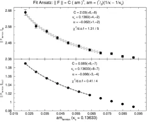
Since we expect the fermion mass to vary in some inverse relation to the norm of the force 关4兴, we attempted to fit the results of our tests with the form
F⫽A共amf兲␣⫽A
冉
1 2⫺
1 2c
冊
␣
, 共61兲
where the parameters of the fit were A,cand␣.
Results of this test are shown in Fig. 7. We show both the fits made to the ⬁-norm and the 共degree of freedom兲 aver-aged 2-norm of the force. We can see that good fits can be made, which reproduce c from the spectroscopic studies
F. Dependence on␦ and
To investigate further the onset of instability, we com-puted the averaged forces and ␦H along an MD trajectory using the same starting configurations as before. However, this time we varied the MD step size ␦. The number of steps taken along the trajectory was adjusted to keep the trajectory length constant at ⫽175/180. The results are plotted in Fig. 8. From the growth of␦H evident in the plot, one can see that the instability sets in between ␦⫽0.0105 and ␦⫽0.0110. We can also see that the rapid growth of ␦H is accompanied by a growth in the fermionic forces in the system共in both norms兲and that the⬁-norm of the force
appears to grow more rapidly than the degree of freedom averaged 2-norm. This latter behavior suggests that the onset of instability is driven by a few unstable fermion modes, again in line with the previous hypothesis.
In a further investigation of the MD forces, we carried out MD trajectories using the same initial gauge configuration as before, this time varying for two separate values of the step size. The values of the step size were ␦⫽0.010 and ␦⫽0.012 corresponding to stable and unstable MD at ⫽0.1355 respectively, as discussed above.
[image:12.612.52.355.59.309.2]We show the⬁-norms of the gauge and fermion forces in Fig. 9. This shows that the simulation which was unstable at FIG. 7. Fits to the fermion force as a function of amf using the fitting hypothesis of Eq.共61兲.
⫽0.1355 has become stable as is reduced. Once again this seems in line with the hypothesis that the onset of the instability is a function of the combination of the fermionic forces共controlled by) and the stepsize␦. Recall that the relevant parameter for the SHO was␦.
Overall, our studies of the MD forces lend support to the hypothesis that the instability is driven by the F␦ term in the momentum update step of the leapfrog algorithm. Since the fermionic force diverges in some inverse relation with the fermion mass, we expect the maximum safe stepsize␦ to decrease as the fermion mass is decreased ( is in-creased兲. Also, having observed a faster rise in the ⬁-norm of the fermionic force than in the degree of freedom aver-aged 2-norm, we infer that the instability is driven by a com-paratively small number of unstable fermionic modes.
V. TUNING THE STEPSIZE AND THE SOLVER RESIDUE
The above conjecture, if correct, can serve to explain the tuning results described in Sec. III G. By increasing the solver residue r, we are modifying the fermionic force which could then drive the MD integrator unstable. In order to in-vestigate these possibilities, we have carried out a second tuning exercise this, time varying both the step size␦ and the solver target residue r.
We used the ten configurations used when tuning r alone in Sec. III G. Since at this point we were not computing Liapunov exponents, our tests consisted of single MD trajec-tories in one direction only. For each value of␦, we chose the number of steps along the trajectory so as to maintain a constant trajectory length of⫽175/180. We also carried out a test with a target residue of r⫽10⫺9using double precision 共64bit兲 floating point numbers, whereas all other tests used single precision. For each combination of algorithmic param-eters, we measured the energy change␦H, the corresponding acceptance probability Paccand the cost function of Eq.共38兲. The results of this tuning exercise are shown in Fig. 10. First we see in the bottom panel (r⫽10⫺9 symbols兲 that using double precision does not alleviate the problem of
in-stability. The calculation in double precision appears to become unstable at a similar value of the step size as does that in single precision. Second, we see from the data for r ⫽5⫻10⫺5 that, if the solver target residue is too large, one cannot achieve values of ␦H of O(1), even if ␦ is made very small.
For our simulations, we are able to achieve non-zero ac-ceptance rates when␦⬍0.0075 and when r⭐10⫺5. For pa-rameter values smaller than these, we can attempt to tune our simulation for maximum performance. The top two panels of Fig. 10 show the variation of the cost function. In this case, the cost function is normalized by its value when r⫽10⫺6 and␦⫽0.0055. These were the parameters used in the pro-duction of the dataset from which the configurations were taken. We see that either by tuning the solver residue r or the MD step size ␦, the maximum gain we could make in the cost function is about 25%.
VI. CONCLUSIONS AND DISCUSSION
A. Stability
We have shown that, for the physical parameters used in our production simulations, the molecular dynamics integra-tor used becomes unstable at␦⬇0.01 for all studied values of r, and also for any realistic value of ␦ when r was in-creased above r⬇O(10⫺5). We identify this instability with the one studied in free field theory for the frequency–step-size combination max␦⫽2. We have studied numerically the fermion force and found that its behavior is not inconsis-tent with the hypothesis of Ref. 关4兴 共motivated by free field theory兲that the force should grow large as→c. We
sup-pose that a critical value exists for F␦ when the leapfrog integrator becomes unstable.
[image:13.612.53.348.57.278.2]parameters, one would need a step-size much smaller than ␦⫽0.001共see Fig. 10兲.
On the safe side of these limits, one may attempt to tune the algorithm. However, our studies show that on this vol-ume and with these physical parameters, tuning␦ and/or r is unlikely to produce significant performance gains. We note that it appears entirely safe to carry out computations in single precision in the safer region of parameter space. How-ever, as→c, it may be that the upper limit on r decreases
beyond the limit of single precision. Alternatively, as the condition number of the fermion matrix increases with in-creasing, the number of iterations in the solver for fixed r will increase. This may cause rounding errors to accumulate so that the target residual r may not be reached. However, in this latter case, it is only the solve itself that needs to be done in double precision, or restarted in single precision.
B. Higher order integration schemes
We have demonstrated that, at least for the case of a simple harmonic oscillator, the fifth and seventh order schemes of Refs. 关6,7兴 are not immune to instabilities. We expect that this situation will persist for even higher order schemes of this sort. The source of the problem is that, at the bottom level, these schemes are constructed out of simple leapfrog updates. For any given step-size␦in an integration scheme of order n⫹3, there will always be a subupdate of order n⫹1 which will have a step-size ␦2⬎␦. This sub-update, or one of its constituent subupdates, may eventually drive the whole integration scheme unstable, although the other subupdates may act as a stabilizing factor at first. We note that, in our harmonic oscillator examples, the smallest positive critical value of ␦ was always smaller for the higher order integrators than for the leapfrog, indicating that the instability problem is actually worse for the higher order methods.
As the source of the instability appears to come from the fermionic part of the force, we anticipate that a scheme of the type advocated in Ref.关8兴would not assist avoiding the
in-stability either, as it attempts to improve the truncation error by performing more gauge updates. While this may drive down the truncation error, it does nothing about the problem in the fermionic update.
C. Reversibility
Reversibility itself seems not to be strongly affected by changing r. The Liapunov exponents of the system seem to show a slow rise before the instability sets in. In the region of transition from stability to instability, the Liapunov expo-nents are difficult to determine. One might speculate that this behavior reflects a transition from the Liapunov exponent characterizing the underlying continuous equations of mo-tion to that characterizing the unstable numerical integrator.
D. Summary
We have investigated the stability and reversibility of the HMC algorithm with two flavors of light dynamical fermions on large lattices as a function of the MD step size␦ and the MD target solver residue r. We have found upper limits on both of these for a fixed set of physical parameters. Beyond these limits, the leapfrog integrator becomes unstable and one cannot carry out a simulation program, irrespective of the precision of the floating point numbers which one uses. On the safe side of the limits, one can carry out simulations safely in both single and double precision. Parameter tuning seems to give no major performance gains. Reversibility does not seem to be dangerously affected.
ACKNOWLEDGMENTS
[image:14.612.55.353.54.279.2]We gratefully acknowledge financial support from PPARC under Grant No. GR/L22744. James Sexton would like to thank Hitachi Dublin Laboratory for support. We also wish to thank Z. Sroczynski for helpful discussions and for his assistance in the preparation of this paper.
FIG. 10. The average energy change 具␦H典, acceptance probability 具Pacc典, and cost function
关1兴S. Duane, A. D. Kennedy, B. J. Pendleton, and D. Roweth, Phys. Lett. B 195, 216共1987兲.
关2兴N. Metropolis, A. W. Rosenbluth, M. N. Rosenbluth, A. H. Teller, and E. Teller, J. Chem. Phys. 21, 1087共1953兲. 关3兴C. Liu, A. Jaster, and K. Jansen, Nucl. Phys. B524, 603
共1998兲.
关4兴R. G. Edwards, I. Horva´th, and A. D. Kennedy, Nucl. Phys.
B484, 375共1997兲.
关5兴Z. Sroczynski, Ph.D. thesis, Edinburgh University, 1998. 关6兴M. Campostrini and P. Rossi, Nucl. Phys. B329, 753共1990兲. 关7兴M. Creutz and A. Gocksch, Phys. Rev. Lett. 63, 9共1989兲. 关8兴J. C. Sexton and D. H. Weingarten, Nucl. Phys. B380, 665
共1992兲.
关9兴B. Sheikholeslami and R. Wohlert, Nucl. Phys. B259, 572 共1985兲.
关10兴K. Jansen and R. Sommer, Nucl. Phys. B 共Proc. Suppl.兲
63A-C, 853共1998兲.
关11兴UKQCD Collaboration, Z. Sroczynski, S. M. Pickles, and S. P. Booth, Nucl. Phys. B共Proc. Suppl.兲63A-C, 949共1998兲. 关12兴M. R. Hestenes and E. Stiefel, J. Res. Natl. Bur. Stand. 49, 409
共1952兲.
关13兴H. van der Vorst, SIAM共Soc. Ind. Appl. Math.兲J. Sci. Stat. Comput. 12, 613共1992兲.
关14兴A. D. Kennedy, Parallel Computing 25, 1311共1999兲. 关15兴C. Moler and C. van Loan, SIAM Rev. 20, 801共1978兲. 关16兴J. C. Sexton et al.共in preparation兲.
关17兴R. Gupta, G. W. Kilcup, and S. R. Sharpe, Phys. Rev. D 38, 1278共1988兲.