Stated choice valuation of traffic related noise

(1)

White Rose Research Online URL for this paper: http://eprints.whiterose.ac.uk/2463/

Article:

Arsenio, A., Bristow, A.L. and Wardman, M.R. (2006) Stated choice valuation of traffic related noise. Transportation Research D, 11 (1). pp. 15-31. ISSN 1361-9209

https://doi.org/10.1016/j.trd.2005.07.001

eprints@whiterose.ac.uk https://eprints.whiterose.ac.uk/ Reuse

See Attached

Takedown

If you consider content in White Rose Research Online to be in breach of UK law, please notify us by

(2)

White Rose Research Online

http://eprints.whiterose.ac.uk/

Institute of Transport Studies University of Leeds

This is an author produced version of a paper published in Transportation Research D. It has been uploaded with the permission of the publisher. It has been refereed but does not include the publisher’s final formatting or pagination.

White Rose Repository URL for this paper: http://eprints.whiterose.ac.uk/2436/

Published paper

Arsenio, A., Bristow, A.L., Wardman, M. R. (2006) Stated Choice Valuation of Traffic Related Noise._{Transportation Research D: Transport & Environment,}

11(1), pp.15-31.

(3)

Stated Choice Valuations of Traffic Related Noise

Elisabete Arsenio

LNEC, Department of Transportation, Lisbon, Portugal

Abigail L. Bristow

Transport Studies Group, Department of Civil and Building Engineering, Loughborough University

Mark Wardman

Institute for Transport Studies, University of Leeds

Corresponding Author: Mark Wardman, Institute for Transport Studies, University of Leeds, Leeds, LS2 9JT, UK.

(4)

Abstract

This paper reports a novel application of the stated choice method to the valuation of road traffic noise. The innovative context used is that of choice between apartments with different levels of traffic noise, view, sunlight and cost with which respondents would be familiar. Stated choice models were developed on both perceived and objective measures of traffic noise, with the former statistically superior, and an extensive econometric analysis has been conducted to assess the nature and extent of householders’ heterogeneity of preferences for noise. This found that random taste variation is appreciable but also identified considerable systematic variation in valuations according to income level, household composition and exposure to noise. Self-selectivity is apparent, whereby those with higher marginal values of noise tend to live in quieter apartments. Sign and reference effects were apparent in the relationship between ratings and objective noise measures, presumably reflecting the non-linear nature of the latter. However, there was no strong support for sign, size or reference effects in the valuations of perceived noise levels.

(5)

1. INTRODUCTION

A recent overview of the state-of-the-art with respect to the economic valuation of noise undertaken for the European Commission (Navrud, 2002) points to the increasing interest in exploring the advantages of stated preference methods to value the environmental externalities of transport. The research reported here provides, alongside other recent papers (Eliasson et al., 2002; Galilea and Ortúzar, 2005; Wardman and Bristow, 2004), a contribution to developments in this area.

Whilst hedonic pricing has been the dominant method in the valuation of transport noise and has the key advantage of being based on actual market choices, it nevertheless suffers from well documented shortcomings (Day 2001; Navrud 2002). Additionally, the method cannot: examine the link between perceived noise levels, objective noise levels and values; identify sign or size effects; explore variations in preferences according to the characteristics of individuals or the response to changes in noise levels; all of which may be important in informing policy choices. These issues are explored here using stated choice.

This paper reports the results of a novel computer based Stated Choice (SC) survey to value traffic noise externalities in Lisbon and is the first attempt to place a value on traffic noise in Portugal. It uses an innovative means of presenting traffic noise to respondents in an SC experiment, building upon research in Edinburgh where a similar approach was used but in the context of air pollution (Wardman and Bristow, 2004). It explores the relationship between measures of perceived noise, which will underpin individuals’ valuations, and the objective noise measures which have to be used in practical appraisals, and reports valuation models estimated to both noise metrics.

The paper is organised as follows. Section 2 discusses issues surrounding the measurement and presentation of traffic noise to respondents and outlines the SC choice context, survey design and data collection process. Section 3 explores the relationship between perceived and measured levels of noise. Section 4 presents the econometric analysis of the SC data and the marginal valuations of noise obtained. This includes: models estimated to both perceived and objective measures of noise; an examination of size, sign and reference effects; the identification of influential variables on marginal valuations; and the estimation of values per unit change in Leq dB(A). Concluding remarks are provided in section 5.

2. SURVEY DESIGN AND DATA COLLECTION

2.1 Presenting Noise Levels in Stated Choice Experiments

The physical units in which noise is normally measured will be meaningless to most people. The issue of presentation therefore becomes more challenging than in more conventional choice contexts and there are several approaches that can be adopted.

(6)

potential problem whilst the scales need to be related to an objective measure of noise. Specifying proportionate changes in noise has been used in valuation studies but respondents have difficulty understanding them and they need to be related to changes to an objective measure. Pictures, photographs and verbal description can be used to describe the environmental good (bad) in question, although this is less suitable for noise than some other forms of externality, and again there will be a problem in linking to an objective measure. Respondents can be exposed to simulated noise in controlled conditions. This is, however, an expensive approach and there is the issue of whether respondents are affected by the artificial and usually limited exposure and how the stimuli relate to respondents’ actual experiences at home. The proxy method presents a variable that respondents can readily relate to and which correlates highly with the externality in question. A suitable variable in this context could be the amount of passing road traffic, although it is questionable whether individuals can correctly interpret the noise levels of different volumes of traffic if they do not actually experience them. What was termed the location method can take a spatial dimension, whereby the respondent is asked to compare different locations with different exposures to environmental impacts, or a temporal dimension, where at the same location there is variation over time.

The location method is an attractive approach provided that suitable contexts can be identified where respondents will be familiar with the noise in the different situations, and the different noise levels are unambiguous and can be measured. In a study of air quality and noise valuations in Edinburgh, Wardman and Bristow (2004) compared the location and proportionate change methods of presenting air pollution within the SC exercise and concluded that the former was preferable. However, they were unable to identify a suitable context in which to apply the method to noise valuation since respondents could not be expected to be familiar with indoor noise levels at different residential locations. The research reported in this paper builds upon that work in using the location method in an SC experiment since the housing market in Lisbon provides a suitable context.

A characteristic feature of the housing market in Lisbon is the presence of apartment buildings located close to major roads but with appreciable variations in noise levels within the same building and lot according to elevation and orientation to the road. Respondents were then presented with traffic related noise levels as experienced and perceived in their own apartments and in other selected apartment situations with which they would generally be familiar. Not only does this context provide a large amount of intrinsically realistic variation, which supports more precise estimates of noise valuations, it avoids extraneous influences by controlling for the quality of the residential area and most apartment characteristics.

It is important that we obtain measures of how noise levels are perceived and how these relate to the objective noise levels. The metrics used in this research were a subjective rating of noise levels on a 0 to 100 scale, with 0 as “very noisy” and 100 as “very quiet”, and Leq dB(A) as the objective measure.

(7)

The context that we identified was that of households’ choices between apartments located within the same building or lot. We offered respondents choices between two different apartment options abstractly composed in terms of the levels of noise, view, sunlight and housing service charge associated with existing apartment locations familiar to respondents. The inclusion of view and exposure to sunlight makes the choice experiment realistic, since these will vary between apartments, and they feature as attributes in information published by estate agents in Lisbon who regard them as decision making variables. They also serve an important role in masking the purpose of the exercise so that respondents do not focus exclusively on noise since it appears as only one of three environmental attributes. Other features of the apartments can reasonably be taken to be the same and indeed this was specified in the experiment.

Some form of payment vehicle needs to be included to allow monetary valuations to be derived. The monthly housing service charge, which covers cleaning and maintenance, was selected since this is a familiar monetary measure whilst typical values are such that sensible variations can be offered consistent with the likely range in which the willingness to pay for the environmental attributes might lie. Reasons for not using the price of the apartment were that the issue of discounting would be involved and the range of sensible monetary valuations would be a very small proportion of the house price. Rent was inappropriate since most apartments were owner occupied. The local property tax in Lisbon is not paid by everyone and it was expected to attract protest responses whilst utility payments reflect use expenditures and are therefore inappropriate.

Respondents were offered a random set of 12 comparisons of apartments A and B from a fractional factorial set of 16 situations. The environmental variables could take four levels relating to:

• The household’s current apartment;

• An apartment on the same floor but on the opposite façade;

• An apartment on a floor either above or below on the same façade; • An apartment on a floor either above or below but on the opposite façade.

The alternative floor was selected to maximise the difference in elevation. This, along with the appreciable differences in noise between the apartments facing the road and those at the back, provides a considerable amount of variation in noise levels which contributes to the precision with which noise valuations can be estimated. Respondents’ perceptions of sunlight and view as well as noise were reported on a rating scale from 0 (very bad) to 100 (very good) for each of the four apartments.

Alternative B was always more expensive and, according to respondents’ ratings, quieter whilst its view and the exposure to sunlight were better than or the same as alternative A. The housing service charge for alternative A was the current charge whilst for alternative B there were four levels which increased the current charge by 15%, 20%, 25% and 35%.

(8)

the current apartment was the quietest then the three other levels appear in alternative A. Where the current apartment was neither noisiest nor quietest, the three largest differences in noise levels were identified and presented.

TABLE 1 ABOUT HERE

2.3 Data Collection

The pilot survey, carried out in April 1999, demonstrated that although respondents did not find the SC choice experiment straightforward, they could relate to comparisons of alternatives composed of features of different apartments, and indicated that the range of cost variations needed to be increased to induce a more satisfactory degree of trading between options. It also revealed that various aspects of wording, presentation and sequencing required amendment.

The main survey took place between June and November 1999 and comprised face-to-face computer assisted interviews at respondents’ homes that yielded 412 valid household responses for modelling purposes. Each respondent was an adult who was asked to represent the household since this is the unit of decision making in the case of residential choice and the environmental attributes would impact on all household members. In the majority of cases, all household members wanted to be present during the interview.

A wide range of background information was also collected to support analysis of variations in noise valuations according to socio-economic, attitudinal, behavioural and locational characteristics whilst physical noise measures were taken indoors and outdoors. The selection of variables was based on review studies of the variables influencing community reactions to traffic noise (Fields, 2001).

The residential area of Telheiras within the Lisbon Metropolitan Area was selected because of the homogeneity of buildings and apartments and the absence of significant confounding noise sources yet variations in exposure to traffic noise and social mix. The main roads nearby have almost continuous traffic levels during the day-time noise reference period (7am-10pm) and traffic noise is the dominant noise source.

The households and apartments surveyed provided rich variation in terms of most attributes. An apartment is classified as ‘Front’ if the bedroom or sitting room is facing the main road. An apartment is classified as ‘Back’ only if both the bedroom and sitting room of the respondent do not face the main road. ‘Lateral’ refers to where no rooms face the front and at least one room is lateral to the main road. The objective of interviewing sufficient numbers of respondents exposed to contrasting noise levels at the front and back and on upper and lower floors was achieved as can be seen in Table 2. The buildings surveyed had between 5 and 11 floors. Further details of the survey design and data collection process are contained in Arsenio (2002).

(9)

The noise data collection comprised indoor and outdoor physical measures at the apartment façade for the upper and lower floors and followed the International Organization for Standardisation Procedures on Acoustics that correspond with the equivalent Portuguese Standard NP 1730 (ISO, 1996).

Table 3 shows the levels of noise rated by the respondents and the corresponding physical noise measures for each apartment exposure type. As expected perceived and measured noise levels are on average higher for apartments which face the road, and higher floors are both perceived and objectively noisier than lower floors. Outdoor measures exceed indoor levels in all cases, reflecting building insulation factors. It is interesting to note that 59% of the householders surveyed had indoor noise levels greater than 35 dB(A), which is the World Health Organization threshold for moderate annoyance and speech intelligibility during the daytime and evening periods (Berglund et al., 1999).

The research reported in this paper aimed to explore the link between perceptions of noise and the corresponding physical noise measures. Table 4 shows the correlations between the differences in ratings and the differences in indoor noise levels for the three comparisons of apartment positions. There is noticeably higher correlation of the subjective and objective measures in the case of front and back comparisons for the same floor (1) and for different floors at opposite façades (3) compared to the noise changes along the same façade (2). The latter weak relationship may well be because of external factors related to the specific housing context such as elevated road sections and the presence of noise barriers.

A more detailed investigation has involved regression analysis of the relationship between the perceived and objective measures of noise. We first estimated a model of the form:

)

( θ θ

α LeqC Leqi

DR= − (1)

DR is the difference in the rating of perceived noise between the current (c) and some alternative (i) apartment which is regressed on the difference in the measured indoor noise levels. Each household contributes three observations based on the comparisons made.

(10)

It emerged that θ was in the range 2.6 to 3.1, depending upon the set of data to which the model was calibrated. The model exhibits the properties of diminishing marginal effects. These are that: a unit increase in Leq would have a bigger impact on ratings than the same reduction (sign effect); a larger change in Leq has a larger unit effect on ratings (size effect); and a unit change in Leq has a larger impact on ratings at higher current levels of Leq (reference effect). However, these relationships are all simultaneously ‘imposed’ by the functional form adopted. We therefore proceeded to examine the presence of the three effects by estimation of a model of the form:

) ( ) ( ) ( ) ( 2 i C C i C i C I i

C Leq d Leq Leq Leq Leq Leq Leq Leq

Leq

DR=α − +β − +γ − +δ −

(2)

The dummy term dI denotes an increase in noise on the current situation and thus

indicates whether any sign effect is present. The squared term indicates whether there is any support for a size effect whilst the final term specifies an interaction with the noise level at the current apartment and tests for the presence of reference effects.

Two models were estimated. One included all three comparisons of apartments per person whilst the other removed situation 2 of Table 4 given the poor relationship between perceived and measured noise levels when apartments on the same façade were compared. The results are presented in Table 5.

TABLE 5 ABOUT HERE.

As expected, the explanatory power increased substantially when observations in situation 2 were removed. There was no statistical support for a size effect but it emerged that an increase in noise had a larger impact on the ratings than an equivalent reduction and that a given change in Leq implied a larger change in ratings when the current apartment was noisier. We introduced a power term on the LeqC interaction in

the final term in equation 2. This would permit the reference effect to be other than proportionally related to the current level of Leq. However, the power term was found to be insignificantly different from one, implying that a proportional effect is justified. The magnitude of the variation is apparent in Table 9 where we subsequently make use of these results to derive monetary valuations of noise expressed in Leq units.

4. STATED CHOICE ANALYSIS

This section reports the findings of the econometric analysis of the SC data comprising 4944 apartment choice observations. This includes:

• estimation and comparison of the performance of models estimated to perceived and objective measures of noise (4.1);

• tests for the presence of size, sign and reference effects (4.2);

(11)

Binary logit choice models were estimated to noise expressed both as a rating and an objective measure. The utility function used to represent the attractiveness of each alternative j within the logit choice model is, for any household i, initially specified as:

ij ij

ij

V

S

N

C

U

=

β

+

η

+

χ

+

γ

(3)

where V, S, N and C represent the levels of view, sunlight exposure, noise and housing service charge respectively in any choice scenario. A mixed logit specification was used (Train et al., 1999) enabling the noise, view and sunlight parameters to vary randomly across respondents. Table 6 reports the models estimated with the GAUSS software and accounting for the correlation in unobserved utility due to the twelve repeated choices by each individual. The maximum simulated likelihood estimation procedure was based on 125 Halton draws, in line with recommendations contained in Bhat (2001).

TABLE 6 ABOUT HERE.

Sunlight and view are in all cases represented by respondents’ rating of them on a scale of 0-100. This scale is also used to represent noise in Models I to IV. Since a higher rating represents an improvement in the attribute in question, the coefficient estimates associated with these ratings should be positive. Costs are expressed in 1999 prices per household per month and have been converted from the escudos used in the SC presentation to Euros1.

The difference between Models I and II is that the former does not allow for the 12 repeated observations per person but the latter and all subsequent models do. This adjustment reduces the t ratios by around 40% on average compared to the treatment of the SC choices simply as independent observations. This contrasts with a reduction of 71% had the repeated choices been assumed to have contained no more information than a single choice.

Model II’s coefficients are all correct sign and statistically significant even at the 1% level. Whilst the goodness of fit measure (ρ2_{) is low, it is not out of line with the figures}

typically achieved by other choice experiments in more conventional contexts such as travel mode or route choice. This is encouraging given the difficult concepts involved.

Model II implies that a unit change in the rating of exposure to sunlight is valued at €1.12 per household per month whilst the equivalent valuation of view is €1.53. It seems plausible that the value of sunlight is lower than the value of view since there is an adverse effect, at least for some people, of sunlight exposure in terms of increasing indoor temperatures to undesirable levels given that most apartments do not have air conditioning.

The value of noise improvements is €1.96 per household per month for a unit change in the rating. It comes as no surprise that a unit change in the rating of noise is more highly valued than the equivalent change in sunlight or view. However, these average values hide a large degree of preference heterogeneity amongst the sample.

1

(12)

Model III allows for random variation in the sunlight, view and noise parameters, in each case following a normal distribution. The standard deviation terms are all highly significant and there has been an appreciable improvement in the goodness of fit. Given the coefficients of discrete choice models are scaled in inverse proportion to the amount of error in the model, there is a corresponding increase in the magnitude of the coefficients. The mean values for sunlight, view and noise are not greatly different from Model II at €1.17, €1.17 and €2.13 respectively. However, the spread of values is large. For example, 95% of the values for noise are in the range -€3.75 to €8.02 and 23.4% of the values within the distribution are negative. Whilst this is not a desirable feature, it is not uncommon that wrong sign valuations are implied when parameters are allowed to follow a normal distribution (Sillano and Ortúzar, 2005; Hess et al., 2005).

Model IV reports the results of a model where the sensitivity to noise follows a lognormal distribution. As expected, we obtained a lower goodness of fit when constraining the model to produce only positive values. The mean noise parameter estimate and its standard deviation are 0.134 and 0.236 respectively2 which leads to a much higher mean value of noise of €3.33 presumably because negative values are not allowed. The asymptotic t-test proposed by Armstrong et al., (2001) was used to compute the 95% confidence intervals of the noise value which range between € 2.22 and €7.31. The mean values of view and sunlight are both lower and close to €0.88.

We turn now to models based instead on objective measures of noise. Model V is a fixed parameters model with the indoor noise from road traffic measured in Leq dB(A). The goodness of fit is noticeably lower when the indoor physical noise measure replaces the ratings. This is to be expected, since the latter more closely reflects individuals’ perceptions of noise and should therefore provide a better explanation of the stated choices. Nonetheless, the noise coefficient, which is now negative as expected, is highly statistically significant. The cost coefficient however becomes insignificant. This is not the result of a different pattern of co-linearity. It presumably stems from the greater error in the model, although this is not reflected in the t ratio associated with view.

Model VI is also based on the indoor objective noise measures but allows the preferences towards the environmental attributes to follow a normal distribution. There is again a large improvement in fit, although it is still inferior to the equivalent ratings model. However, once again wrong sign valuations of noise would be implied: in this case for 26.0% of the sample. When we tried to specify the noise coefficient as lognormally distributed, model convergence could not be achieved. This result is perhaps unsurprising given that there is no outlet for the apparently wrong sign coefficients.

The outdoor noise measure used in Model VII provides, as expected, a worse account of choices than the indoor noise measures given that the former will be an even poorer approximation to the noise levels experienced by residents in their homes. The cost coefficient is far from statistically significant in this model.

(13)

We here explore whether departures from the linear-additive utility function of equation 3 can be justified, specifically testing whether valuations based on respondents’ ratings are subject to sign, size or reference effects.

It is a simple matter to test whether gains and losses are valued differently by specifying alternative specific noise coefficients since alternative A is always noisier than or the same as the rated household apartment and alternative B is quieter or the same. When such a model was specified, the coefficient for increases in noise was 0.0350 (t=7.6) and for reductions was 0.0318 (t=8.4). The former is only 10% larger than the latter and, with a t ratio of 1.6, the difference is not quite statistically significant.

As far as size effects are concerned, we specified noise in the following form for the two alternatives:

2 )

( _C _A

A

A N N N

U =β +α − (4a)

2 )

( _B _C

B

B N N N

U =β +α − (4b)

where NC is the current level of noise at each household’s apartment. The marginal

utilities are then:

(

C A

)

A

A N N N

U ∂ = + −

∂ / β 2α (5a)

(

B C B

B N N N

U ∂ = + −

)

∂ / β 2α (5b)

Given that alternative A involves increases in noise from the current level experienced by households and alternative B involves reductions, this specification forces the same incremental effect from the size of a change regardless of whether a gain or loss is concerned.

The term was -0.000097 which implies a diminishing sensitivity to larger changes which is consistent with the reference dependent preference theory of Tversky and Kahneman (1991). However, the effect is small and, with a t statistic of 1.55, it was not statistically significant.

We also specified an incremental term to test whether the valuation of noise depended on the level of noise. This took the form:

C A A

A N N N

U =β +α (6a)

C B B

B N N N

U =β +α (6b)

whereupon the marginal utilities are + NC. The coefficient was 0.000119 but with a t

(14)

somewhat worse fit was obtained. We therefore conclude that the unit valuation of noise is independent of the level of noise.

Not only are size and sign effects not present for noise valuations, but we also tested for these analogous effects in the cost coefficients and they were negligible.

4.3 Influential Variables

Although random taste variation is permitted in some of the models in Table 6, we now turn to the issue of systematic taste variation. We have enhanced Models II and III to incorporate systematic variations in preferences according to the socio-economic and contextual characteristics of the respondent and household. This is a standard procedure, involving the specification of dummy variable interaction terms to estimate a range of incremental effects on the weights attached to noise and cost. For example, we could specify dummy variables for whether the apartment was located at the back of the block (d1) or lateral (d2) whereupon the utility function becomes:

ij ij ij ij ij ij

ij V S N C d N d N

U =β +η +χ +γ +α ₁ +λ ₂ (7)

The sensitivity to noise for apartments at the front is χ whilst it is χ+α for apartments at the back and χ+λ for lateral apartments.

The possible sources of systematic preference variation were: household income, size and composition; exposure to noise; current level of annoyance with noise; floor level and position of the apartment relative to the main road; averting noise behaviour; age, gender and educational attainment of the respondent; the degree of familiarity with the alternative apartments used in the SC exercise; awareness of the health impacts of noise; whether the windows were usually open in Spring and Summer; years of residency; the presence of noise barriers; and the class of main road following the functional road hierarchy.

(15)

We expect that as households become wealthier and therefore less sensitive to cost variations, the amount that they are prepared to pay for improvements in noise or indeed any other attribute will increase. When separate cost coefficients were estimated for different income groups, this demonstrated an income effect of the expected form. We therefore proceeded to estimate a continuous function relating the monetary values through the cost coefficient to the level of income. Two measures of income were tested. One was calculated taking the mid-point of each income category. The other was adjusted household income per person, obtained by dividing the estimated monthly household income by a scale factor that considered the effect of household composition using the equivalisation procedure of the UK Department of Social Security (DSS, 1998). The cost term was entered into the utility function as:

λ γ

Y C

U = (8)

The marginal utility of money will fall and monetary values will increase as income increases, and λ denotes the elasticity of the marginal value of noise with respect to income.

It emerged that adjusted household income per person provided a better fit than household income or unweighted household income per person. The search process across different values of λ identified the best fitting model to be for an income elasticity of 0.5, and this is very much in line with other evidence (Wardman and Bristow, 2004).

The only two statistically significant effects on noise in Model VIII relate to whether the household lived at the back of the apartment away from the road (NOISE-BACK) or they lived on an upper floor (NOISE-FLOOR).

Householders located at the back have a much higher sensitivity to noise. This is a self-selectivity effect, whereupon those with higher values choose to live in quieter locations, and the effect is appreciable, an effect also found by Eliasson et al., (2002). For example, ignoring the floor effect, those living at the back have values of noise that are over twice as high as those located at the front, all other things equal.

Householders who live on upper floors have a higher valuation of quiet than those who live on lower floors, ceteris paribus, although a monotonic increasing effect could not be obtained. The best fit was found when upper floors were specified as a dummy variable for households located above the fourth floor. Again the incremental effect is large. Whilst it could not be claimed self selectivity is having an influence here, because as we have seen apartments on higher floors are on average noisier, this might not have been the preconception when the apartment was purchased.

(16)

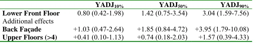
Although we could only discern a few sources of systematic taste variation, there is considerable variation across the sample according to these factors. For example, a household with adjusted income at the 10th percentile and living on a lower floor at the front has a value of noise of €0.80 per unit change in rating per month whereas for those with adjusted income equal to the 90th percentile and living at the back on an upper floor the mean valuation is €8.56.

The absence of more variables having a systematic influence on values could be due to a failure to fully capture the dynamics of household decision making and further exploration of this issue is needed. However, to the extent that different respondents use the rating scales differently, this may lead to more random variation at the expense of detectable systematic variation.

4.4 Values per Decibel

It is useful to express values in terms of Leq for comparison with the results of other studies and for easier practical application in Cost-Benefit Analysis since an objective noise exposure, even indoors, can be estimated for current and future years. We have used the model in the final column of Table 5 which relates changes in ratings (DR) to changes in Leq in the form:

) (

0576 . 0 ) (

8904 .

0 dI LeqC Leqi LeqC LeqC Leqi

DR=− − − − (9)

where dI denotes an increase in noise on the current situation and Leq is the measured

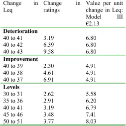
indoor noise level for the current (c) and alternative (i) apartment. Table 9 reports the changes in ratings for a range of Leq variations and levels and demonstrates the sign and reference effects previously estimated. These are then converted into valuations of a unit change in Leq using the mean valuation of €2.13 per unit change in rating from Model III.

For a typical measurement at the current apartment of 35 Leq dB(A), a decrease of one Leq db(A) would be equivalent on average to a change of 2.02 units in perceived noise rating giving a value of €4.30 per household per month per dB(A) or €51.60 per year. The corresponding figure for a unit increase in Leq dB(A) would be €74.30. These figures seem plausible. Note that although we could in principle use models estimated to Leq to derive noise valuations in units of Leq, as with Models V and VI of Table 6, the cost coefficients in those models were not statistically significant and hence the implied monetary values would not be reliable.

5. CONCLUSIONS

(17)

factor will have been the use of a choice context centred around apartments with different noise levels which respondent would generally be familiar with.

Households rated the perceived noise levels associated with different apartments on a 0-100 scale. These ratings were related to objective indoor noise measures based on Leq dB(A) which found that there was reference effect, whereby a given change in objective noise was perceived to be noisier when it occurred at higher levels of Leq, and a sign effect, where deteriorations had a larger impact than improvements. This presumably represents the non-linear nature of the objective measure.

A wide range of possible key influential variables on the valuation of noise was tested and a number of interesting findings emerged. Firstly, there was no strong statistical support for size, sign or reference effects in models calibrated to perceived noise levels as represented by ratings. This is in line with the findings of Wardman and Bristow (2004) who conducted similar analysis of Stated Choice data for noise and air quality but is at odds with findings commonly obtained. Secondly, random taste variation was found to be appreciable, and allowing for it considerably improved the explanatory power of the models. Thirdly, whilst systematic variations in preferences were only detected with regard to income, household composition and exposure to traffic noise, and these provide a lesser explanation of choices than allowing for random variation, they would still imply considerable variation in valuations across the population. The income elasticity was found to be 0.5, in line with other studies of traffic noise. The strong variations in values with exposure imply a self-selectivity effect. This finding suggests that the common use of a cut-off level of noise below which no annoyance or cost is deemed to occur may be inappropriate as it will undervalue the preferences of those in quiet areas who are willing to pay relatively large amounts to preserve that quiet.

The Stated Choice models based on perceived noise are clearly superior to those based on objective measures of noise. The values for a change in noise rating are then converted to a value for a change in Leq through the modelled relationship between perceived and objective noise. These models then have the potential for practical application in transport and environmental policy impact assessment and appraisal. There is clearly scope for further research to refine the Stated Choice methodology and undertake comparative studies of Revealed and Stated Choice techniques.

REFERENCES

Arsenio, E. (2002). The Valuation of Environmental Externalities: a Stated Preference Case Study on Traffic Noise in Lisbon. PhD Thesis, Institute for Transport Studies, University of Leeds, UK.

Armstrong, P. M. Garrido, R. A. Ortuzar, J. de D. (2001) Confidence Intervals to Bound the Value of Time. Transportation Research Part E 37, 143:161.

(18)

Bhat, C. (2001) Quasi-random maximum simulated likelihood estimation of the mixed multinomial logit model, Transportation Research Part B 35: 677-693.

Day B. (2001) The Theory of Hedonic Markets: Obtaining welfare measures for changes in environmental quality using hedonic market data. Economics for the Environment Consultancy.

Department of Social Security (1998) Households Below Average Income 1979-1966/7, A.Grait: Grimsby.

Eliasson J., Lindqvist Dillen J. and Widell J. (2002) Measuring Intrusion Valuations Through Stated Preference and Hedonic Prices: A Comparative Study. Paper Presented to European Transport Conference, PTRC, London.

Fields, J. (2001) An Updated Catalog of 521 Social Surveys of Residents’ Reactions to Environmental Noise (1943-2000). NASA/CR-2001-211257, Washington, D.C.: National Aeronautics and Space Administration.

Galilea, P. and Ortúzar, J. de D. (2005) Valuing Noise Level Reductions in a Residential Location Context. Transportation Research D 10(4) 305-322.

Hess, S. Bierlaire, M. Polak, J. (2005) Estimation of value of travel-time savings using mixed logit models. Transportation Research Part A. 39(2/3), 221:236

ISO-International Organization for Standardization (1996) Acoustics- Description, measurement and assessment of environmental noise: basic quantities and assessment procedures (Part 1) and Acquisition of data pertinent to land use (Part 2), Geneva, Switzerland.

Navrud, S. (2002) The State-of-the-Art on Economic Valuation of Noise. Final report to the European Commission, DG Environment.

Sillano, M. Ortuzar, J. de D. (2005) Willingness-to-pay estimation with mixed logit models: some new evidence. Environment and Planning A.37 525:550

Train, K. Revelt, D. Ruud, P. (1999) Mixed Logit Estimation Routine for Panel Data.

http://emlab.berkeley.edu/softaware/

Tversky, A. and Kahneman, D. (1991) Loss Aversion in Riskless Choice: A Reference-Dependent Model. The Quarterly Journal of Economics106 (4), 1039:1061.

Wardman, M. and Bristow, A.L. (2004) Traffic related noise and air quality valuations: evidence from stated preference residential choice models. Transportation Research

(19)

[image:19.595.85.347.97.219.2]

Table 1: Noise Levels in the SC Experiment

Current Apartment

Alternative A Alternative B

Noisiest Noisiest Quietest 2nd Quietest 2nd Noisiest 2nd Noisiest

2nd Quietest

Noisiest 2nd Noisiest

Quietest 2nd Quietest Quietest Noisiest

2nd Noisiest 2nd Quietest

(20)

Table 2: General Exposure and Apartment Location

(21)

[image:21.595.89.512.126.364.2]

Table 3: Mean Levels of Ratings and Physical Measures of Noise (Standard errors in parentheses)

Exposure and floor number

Mean Rating

Mean Leq dB(A)

Indoors

Mean Leq dB(A) outdoors FRONT to main road (242)

1-3 Barrier (40) 54.65 (2.97) 35.92 (0.55) 64.46 (0.66) 1-3 No Barrier (81) 43.15 (3.00) 36.97 (0.57) 65.30 (0.55) 4-6 (90) 39.80 (2.64) 39.19 (0.40) 67.23 (0.56) 7+ (31) 36.48 (4.35) 40.87 (0.89) 69.17 (0.71) BACK to main road (133)

1-3 Barrier (19) 58.33 (3.62) 35.17 (0.78) 63.60 (0.70) 1-3 No Barrier (41) 63.34 (3.20) 33.17 (0.59) 63.03 (0.77) 4-6 (39) 57.10 (3.02) 35.33 (0.66) 63.80 (0.74) 7+ (34) 60.15 (2.84) 34.24 (0.79) 65.20 (0.72) LATERAL to main road (37)

1-3 Barrier (8) 50.80 (9.67) 34.10 (1.30) 64.40 (2.66) 1-3 No Barrier (12) 43.33 (7.56) 36.70 (1.54) 60.84 (2.97) 4-6 (16)

7+ (1)

54.44 (4.58) 9.00 (0.00)

35.06 (1.13) 41.00 (0.00)

(22)

[image:22.595.87.516.92.255.2]

Table 4: Correlations Between Perceived and Actual Differences in Noise Levels

1

2

3

Front - Back façade, same floor

-0.568, p=0.000 - -

Lower-Upper floor, same façade

- -0.147, p=0.003

Lower-Upper floor, opposite façade

- -0.533, p=0.000

(23)

[image:23.595.80.371.99.189.2]

Table 5 Regression Models of Ratings on Leq dB(A) measures

Parameters All 1 and 3

α 3.2470 (5.26) n.s.

β (Sign Effect) -1.0334 (4.77) -0.8904 (4.88) δ (Reference Effect)) -0.1261 (7.54) -0.0576 (18.35)

Adj R2 0.195 0.460

(24)

Ratings Fixed Parameters

Ratings Random Parameter

Ratings Random Parameters

Indoor Noise Fixed Parameters

Indoor Noise Random Parameters

Outdoor Noise Fixed Parameters

VIEW – Mean 0.0243 (13.7) 0.0243 (9.4) 0.0371 (8.4) 0.0353 (8.7) 0.0278 (10.8) 0.0431 (10.9) 0.0284 (11.1) VIEW – SD - - 0.0417 (6.4) 0.0522 (8.5) - 0.0457 (7.8)

SUN – Mean 0.0178 (10.6) 0.0178 (6.2) 0.0370 (6.5) 0.0351 (7.2) 0.0152 (5.6) 0.0339 (6.5) 0.0152 (5.5) SUN – SD - - 0.0643 (6.7) 0.0563 (8.4) - 0.0538 (6.5)

NOISE – Mean (N) 0.0311 (15.9) 0.0311 (8.4) 0.0674 (9.4) - -0.0585 (6.2) -0.1035 (6.0) -0.0501 (5.5) NOISE – SD (N) - - 0.0930 (8.6) - - 0.2562 (7.7) -

NOISE – Mean (LN) - - - -3.0769* (23.3) - - -

NOISE – SD (LN) - - - 1.4611* (11.2) - - -

COST (€) -0.0159 (5.0) -0.0159 (3.0) -0.0316 (3.8) -0.0402 (4.4) -0.0062 (1.2) -0.0074 (1.1) -0.0039 (0.8) Log Likelihood

ρ2

-2915.3 0.088

-2521.9 0.211

-2550.9 0.202

-3022.0 0.055

-2657.4 0.169

[image:24.842.66.702.96.283.2]

(25)

[image:25.595.90.406.128.317.2]

Table 7: Examination of Systematic Taste Variation

VIII IX

VIEW - Mean 0.0366 (9.3) 0.0432 (9.2) VIEW – SD 0.0439 (7.1) 0.0645 (8.9) SUN – Mean 0.0366 (7.3) 0.0337 (7.0) SUN – SD 0.0603 (8.4) 0.0608 (10.3) NOISE – Mean (N) 0.0450 (6.3) 0.0297 (6.0) NOISE – SD (N) 0.0871 (9.9) - COST/YADJ 0.5 -0.4720 (4.0) -0.3071 (2.9) COST-MISS -0.0357 (2.9) -0.0317 (2.7) NOISE-BACK 0.0583 (4.8) 0.0357 (3.6) NOISE-FLOOR

NOISE-FEMALE NOISE-LENGTH NOISE-LOT

0.0232 (3.1) - - -

0.0155 (2.1) 0.010 (1.6) -0.0135 (2.1) -0.0097 (1.7) Log Likelihood -2502 .3 -2611.4

ρ2 _0.217 _0.183

Note: The units of NOISE, VIEW and SUN are the 0-100 ratings;

(26)

[image:26.595.86.519.114.188.2]

Table 8: Household Monthly Valuations of Noise (€)

YADJ10% YADJ50% YADJ90%

Lower Front Floor 0.80 (0.42-1.98) 1.42 (0.75-3.54) 3.04 (1.59-7.56)

Additional effects

Back Façade +1.03 (0.47-2.64) +1.85 (0.84-4.72) +3.95 (1.79-10.08)