The identification of coupled map lattice models for autonomous cellular neural network patterns

This is a repository copy of The identification of coupled map lattice models for autonomous cellular neural network patterns.

White Rose Research Online URL for this paper: http://eprints.whiterose.ac.uk/74608/

Monograph:

Pan, Y., Billings, S.A. and Zhao, Y. (2007) The identification of coupled map lattice models for autonomous cellular neural network patterns. Research Report. ACSE Research Report no. 949 . Automatic Control and Systems Engineering, University of Sheffield

Reuse

Unless indicated otherwise, fulltext items are protected by copyright with all rights reserved. The copyright exception in section 29 of the Copyright, Designs and Patents Act 1988 allows the making of a single copy solely for the purpose of non-commercial research or private study within the limits of fair dealing. The publisher or other rights-holder may allow further reproduction and re-use of this version - refer to the White Rose Research Online record for this item. Where records identify the publisher as the copyright holder, users can verify any specific terms of use on the publisher’s website.

Takedown

If you consider content in White Rose Research Online to be in breach of UK law, please notify us by

ｔｨ･＠ｉ､･ｮｴｩｦｩ｣｡ｴｩｯｮ＠ｯｦ＠ｃｯｵｰｬ･､＠ｍ｡ｰ＠ｌ｡ｴｴｩ｣･＠ｭｯ､･ｬｳ＠ｦｯｲ

ａｵｴｯｮｯｭｯｵｳ＠ｃ･ｬｬｵｬ｡ｲ＠ｎ･ｵｲ｡ｬ＠ｎ･ｴｷｯｲｫ＠ｐ｡ｴｴ･ｲｮｳ

ｐ｡ｮＬ＠ｙＮＬ＠ｂｩｬｬｩｮｧｳＬ＠ｓＮ＠ａＮ＠｡ｮ､＠ｚｨ｡ｯＬ＠ｙＮ

ｄ･ｰ｡ｲｴｭ･ｮｴ＠ｯｦ＠ａｵｴｯｭ｡ｴｩ｣＠ｃｯｮｴｲｯｬ＠｡ｮ､＠ｓｹｳｴ･ｭｳ＠ｅｮｧｩｮ･･ｲｩｮｧ

ｕｮｩｶ･ｲｳｩｴｹ＠ｯｦ＠ｓｨ･ｦｦｩ･ｬ､

ｓｨ･ｦｦｩ･ｬ､Ｌ＠ｓＱ＠Ｓｊｄ

ｕｋ

The Identification of Coupled Map Lattice

models for Autonomous Cellular Neural

Network Patterns

Pan, Y., Billings, S. A. and Zhao, Y.

Department of Automatic Control & Systems Engineering

Sheffield University,

Sheffield, S1 3JD, UK

March, 2007

Abstract

The identification problem for spatiotemporal patterns which are generated by autonomous Cellular Neural Networks (CNN) is inves-tigated in this paper. The application of traditional identification algorithms to these special spatiotemporal systems can produce poor models due to the inherent piecewise nonlinear structure of CNN. To solve this problem, a new type of Coupled Map Lattice model with output constraints and corresponding identification algorithms are proposed in the present study. Numerical examples show that the identified CML models have good prediction capabilities even over the long term and the main dynamics of the original patterns appears to be well represented.

1

Introduction

have been observed in biological systems [18]. As a consequence of the com-mon occurrence of spatial patterns, the discovery of new pattern formation phenomenon is potentially of great research interest. Several authors have therefore studied the analysis and simulation of a variety of spatiotempo-ral models which produce various interesting spatial patterns. The Partial Differential Equation (PDE) models where the variables evolve continuously over the continuous space and time domain have been used to describe a wide class of spatiotemporal behaviours, including the Gray-Scott model [11], Fitz-Hugh-Nagumo model and Belousov-Zhabotinsky model.

Cellular Neural Networks (CNN) [7] which are defined by the coupling of cells continuously evolving over a discrete spatial lattice have also been widely applied to model complex spatiotemporal patterns. Because of the simplicity and easy implementation in hardware, CNN’s have found numerous applica-tions in image and video signal processing, and in pattern recognition. Apart from providing an alternative paradigm for simulating nonlinear Partial dif-ferential Equations, CNN models have been shown to generate propagating waves, patches, checkerboard patterns, stripes and reaction-diffusion type patterns [2] [23] [13]. Further research on the emergence and complexity of spatiotemporal systems has revealed that CNN can give rise to many inter-esting patterns by tuning the parameters in the CNN templates. Hence, the problem of deriving the corresponding CNN templates for specific spatiotem-poral behaviours has also been recently investigated [13].

The Coupled Map Lattice model which was initially introduced in the 1980s by Kaneko [14][15] has been widely used to model spatiotemporal sys-tems. The CML model is discrete in time and space and has a continuous state value. A CML is a d-dimension lattice where each site evolves in time through a discrete map which describes the influence of the past state and neighboring sites. It has been shown that CML models can exhibit complex spatiotemporal behaviors, including chaos, intermittency, travelling waves and Turing patterns [16]. Compared with PDE models, CML models are computationally more efficient and have been used to study spatiotemporal systems in a wide class of scientific subjects.

coefficients of the identified model are adjusted by using an amended error sequence from the model prediction to enhance the prediction performance of the final model.

The paper is arranged as follows. Section 2 gives a general description of autonomous Cellular Neural Networks and Coupled Map Lattice models for spatiotemporal systems. Section 3 introduces a correlation based method to select the sampling interval for the identification data. Then, the new iden-tification method which is based on a modified OFR algorithm is proposed. Some numerical examples of CNN patterns are included in Section 4 to illus-trate the application of the new identification methods and to demonsillus-trate the performance of the identified CML models to identify these systems.

2

Autonomous Cellular Neural Networks and

Coupled Map Lattice Models

2.1

Coupled Map Lattice models

Consider the input-output CML model for time and spatially invariant spa-tiotemporal systems[8] [9]

yi(k) =f(qnyyi(k), qnuui(k), qnysmyyi(k), qnusmuui(k)) +εi(k) (1)

where i _∈ Id _{is the spatial index of a d-dimensional space and k = 1,2, . . . ,}

is the temporal index; yi(k), ui(k) and εi(k) are the output, input, model

residual sequences respectively, andqn_{(k) is a temporal backward shift}

oper-ator

qn = (q−1_{, q}−2_{, ..., q}−n

) (2)

so that

qny_y

i(k) = (yi(k−1), yi(k−2), ..., yi(k−ny))

qnuu

i(k) = (ui(k−1), ui(k−2), ..., ui(k−nu)) (3)

In (1), sm _{is a multi valued spatial shift operator}

sm= (sp1, sp2, ..., spm) (4)

where pj _∈Id _{is the spatial translation multi index, such that}

smy_y

i = (yi−p1, y_i−p2, ..., y_i−pmy)

smu_u

i = (ui−p1, u_i−p2, ..., ui−pmu) (5)

The parameters my, mu denote the maximum spatial radius associated with

2.2

Autonomous Cellular Neural Networks

A CNN is said to be autonomous if the cells do not have external inputs. The standard form of an autonomous CNN defined over a two dimensional

N _×N array can be expressed by the following equation,

˙

xi,j =−xi,j+zi,j + X

n,l∈Si,j

an,lyn,l (6a)

yi,j =g(xi,j) (6b)

where (i, j) _∈ N _×N denotes the spatial site and xi,j, yi,j are state space

variables and output variables respectively. The output function g(_·) here is defined as the three segment piecewise linear saturation function.

g(xi,j) =

1

2(|xi,j + 1| − |xi,j−1|) (7) The CNN dynamics are usually restricted to be inside the boundary of the array N _×N. Consequently, additional boundary conditions need to be specified for model (6). Three kinds of boundary conditions are most com-monly used, Dirichlet (fixed), Neumann (zero flux) and Toroidal (periodic) boundary conditions. With specific boundary conditions, the dynamics of the standard CNN (6) is then only determined by the CNN template which is composed of the threshold zi,j and the neighbourhood coupling matrix

A =_{an,l}. If the neighbourhood radius of every cell is set to be r = 1, the

feedback template A of a two dimensional CNN can be described as follows.

A=





a−1,−1 a−1,0 a−1,1

a0,−1 a0,0 a0,1

a1,−1 a1,0 a1,1 

 (8)

The behaviours of different pattern formations of standard autonomous CNN models have been extensively studied with various A-templates using state space stability theory. Perturbing the unstable equilibrium state with small and random disturbances, the symmetry of the unstable equilibrium is broken and complex patterns will be formed. As can be seen from the piecewise func-tion g(_·), the output trajectories of all cells can be divided into three regions: a linear region and two saturation regions. Because the output functiong(_·) is continuous and bounded, all trajectories defined by the standard CNN model (6) will converge to an equilibrium state when certain conditions are satisfied [7].

of sampled continuous time CNN patterns. Generally, the form of the CML model f(_·) is unknown, so it is necessary to expand f using a known set of possible candidate model terms. Equation (1) can also be written in a regres-sion format which is constructed as a linear combination of a finite number of model terms.

yi(k) = X

k

θi,mϕi,m(k) +εi(k) (9)

Here, model terms ϕi,m(k) are composed of qnyyi(k), qnuui(k), qnysmyyi(k),

qnusmuu

i(k) which represent the influence of past inputs and outputs from

both the local and neighboring lattices.

3

A CML Identification Algorithm for

Cellu-lar Neural Network Patterns

3.1

The selection of the sampling interval for the

iden-tification data

The selection of the sampling interval of the original continuous data in sys-tem identification could have a great influence on the term structure selection and parameter estimation of the identified model. For example, if the iden-tification data is over-sampled, the regression matrix will become ill-posed due to the high correlation between successive measurements. On the other hand, if the data for identification is under-sampled, important dynamic in-formation will be lost. In these situations, the final derived model is more likely to be ill-posed and sensitive to new training data or to noise.

The sampling time of the identification data from the CNN patterns which are continuously evolving over a discrete lattice needs to be appropriately determined to ensure the regression matrix is well defined. In this section, a correlation function based method [4] [6] [22] will be used to select an appropriate sampling procedure. Compared with other methods which are mostly based on information theoretical tools, the correlation method is quite simple and robust to noise. The main concept behind this method is to select proper time intervals so that the dynamic information in the patterns are retained in the identification data.

The selection procedure for the sampling time is based on the linear and nonlinear functions defined as follows.

Φyy(τ) =

PS(Ns−1)

(i,k)=S(0)(yi(k)−y)(yi(k−τ)−y) PS(Ns−1)

(i,k)=S(0)(yi(k)−y)2

Φy2_y2(τ) =

PS(Ns−1)

(i,k)=S(0)(yi2(k)−y2)(yi2(k−τ)−y2) PS(Ns−1)

(i,k)=S(0)(yi2(k)−y2)2

(10b)

In (10), Ns samples of the original spatiotemporal data is collected from

outputs that are randomly selected over both the space and time domain, and _· denotes the averaging operation over the specific domain defined by the selection vector S. On the basis of the above equations, both the linear and nonlinear correlation relationships of the data can therefore be measured. The minimum time values associated with the correlation functions can be defined.

τm =min{τy, τy2} (11)

where τy and τy2 are time values of the first minimum of φyy(τ) andφy2_y2(τ)

respectively. In practice, the 95% confidence limits which are equal to

±1.96/√Ns are usually used to replace the minimum values of the above

correlation functions

The sampling intervals T for the spatiotemporal data in the time domain [1] can be chosen by following the rule of thumb.

τm

20 ≤T ≤

τm

10 (12)

In practical applications, this simple but effective empirical method appears to work well.

3.2

The identification algorithm

The identification problem for spatiotemporal systems is composed of two parts: model term selection and parameter estimation. The Orthogonal Forward Regression (OFR) algorithm which involves a stepwise orthogonali-sation of the regressors and a forward selection of the significant terms based on the Error Reduction Ratio (ERR) criterion [5] has been successfully ap-plied to identify a wide class of spatiotemporal systems [8] [9] [12]. Using this method, the model structure is selected step by step by comparing the ERRs of all possible model terms from a set of candidate regressors _{ϕm}Mm=1

Functions, Kernel Basis Functions, Polynomials and Wavelets) which are currently widely used in model identification.

In this section, a new identification method for autonomous CNN patterns is proposed to solve this problem. The format of the revised CML model for CNN pattern identification is defined as follows.

yi(k) =g(f′(qnyyi(k), qnysmyyi(k))) +εi(k) (13)

The function g(_·) is the same as defined in (7). The incorporation of the functiong(_·) ensures that the output of the identified CML model will evolve within a certain region. The main aim of identifying the CML model for CNN patterns is then to determine the unknown function f′

(_·) in (13). The two corresponding One-Step-Ahead (OSA) prediction errors associ-ated with function f′₍

·) in (13) can be expressed as

ε(iosa)(k) = yi(k)−yi(osa)(k) = yi(k)−g(f′(qnyyi(k), qnysmyyi(k)))(14)

ε′(osa)

i (k) = yi(k)−y

′(osa)

i (k) = yi(k)−f′(qnyyi(k), qnysmyyi(k)) (15)

where εi(k) is the actual OSA prediction error andε′i(k) is the original OSA

prediction error without considering the impact of the output function g(_·). It is well known that the OFR identification method is a least squares based algorithm and the aim of traditional CML identification algorithm is to obtain a final CML model based on the sum of the squared OSA prediction error P

i,kε2i(k). The ERR can be expressed as

ERRm =

g2

mwTmwm

YT_Y , gm=

wT mY

wT mwm

(16)

where wm is the orthogonalised regressor associated with term ϕm andgm is

the corresponding estimated coefficient. However, when the standard OFR algorithm is applied to obtain the model f′

(_·) in (13), it can be easily seen from (16) that the influence of the nonlinear output functiong(_·) is not taken into account during the ERR computation. For example, when yi(k) = 1

and y′(osa)

i =f

′_(qnyy

i(k), qnysmyyi(k)) > 1, the actual OSA prediction error

εi(k) in (14) should be 0 but ε′i(k) will not be equal to 0 when the output

function g(_·) is not taken into account. In this situation, ERR which is used to measure the proportional contribution of each term to the variance of the overall dependent variables may provide incorrect information for term selection. Similar problems would also arise during the computation of the associated coefficients.

selected step by step by comparing the sum of the squared OSA prediction error P

i,kε

2

i(k) during every orthogonalisation stage. The estimates of the

corresponding coefficients are then adjusted using the updated output vector according to the nonlinear function g(_·).

In summary, the amended OFR algorithm for identifying this class of CNN patterns is outlined as below.

Step j=1: Select the first model term with the smallest prediction error

I1 =IM ={1,2, ..., M}, Y1 =Y (17)

wi(k) = ϕi(k),ˆbi =

[wi, Yi]

[wi, wi]

(18)

Find the term with the smallest prediction error.

l1 =argmin

i∈I1

³

YT

1 Y1−ˆb2iw T i wi

´

(19)

Compute the coefficient of the selected term.

p1 =wl1, c1 =

[p1, Y1]

[p1, p1]

, a1,1 = 1 (20)

Update the output vector Y2 according to the first model prediction.

y1(osa)(k) =c1∗p1(k)

If _|y1(osa)(k)|>1,then

y2(k) = y1(osa)(k),

else

y2(k) = y1(k), k= 1,2, . . . , N

Stepj,j = 2,3, ...: Iteratively orthogonalise the remaining regressors one by one to select the next model term with the smallest prediction error among the remaining candidate terms.

Ij =Ij−1\lj −1 (21)

Orthogonalise the model regressors.

wi(k) = ϕi(k)− j−1

X

m=1

[pm, Yj]pm

[pm, pm]

,ˆbi =

[wi, Yj]

[wi, wi]

(22)

Find the model term with the smallest prediction error.

lj =argmin i∈Ij

Ã

YT j Yj −

j−1

X

m=1

c2mpTmpm−wTi wi !

Compute the coefficient of the selected term.

pj =wlj, cj =

[pj, Yj]

[pj, pj]

, am,j =

[pm, ϕlj]

[pm, pm]

, m = 1,2, ..., j₋1 (24)

Update the output vector Yj+1 according to the model prediction at stage j.

y_j(osa)(k) =

j X

m=1

cm∗pm(k)

If _|y_j(osa)(k)_|>1, then

yj+1(k) =yj(osa)(k),

else if yj(k)>1,

yj+1(k) = 1

else

yj+1(k) = yj(k), k = 1,2, . . . , N

This procedure is terminated at the Ms-th step when a required number

of terms has been selected in the final model. The estimated coefficients Θ = _{θm}mm=1=Ms associated with the selected terms{ϕlm}

m=Ms

m=1 are computed

using

Θ =A−1_{C, (25)}

where A =_{am,j} is an upper-triangular matrix which is defined above and

C = (c1, c2, ..., cMs) is the coefficient vector associated with the

orthogo-nalised terms _{pm}Mm=1s .

In this new model identification algorithm, the summation of squared one-step-ahead prediction errors associated with every term selection is employed as a criterion for model term selection. The values of the one-step-ahead pre-diction error and term coefficients at each step are adjusted by updating the output vector when the output prediction falls within the saturation region associated with the definitions of the CNN models. Using this approach, the prediction performance of the identified model can be greatly improved.

4

Numerical Examples

stable equilibrium state. The proposed CML model (13) and the identifica-tion algorithm described above were then applied. In these examples, the model predicted output was simulated to test the prediction performance and dynamical characteristics of the new identified CML model. The model predicted output y(_i,jmpo)(k) is defined as follows,

yi,j(mpo)(k) =g(f

′

(qny_y(mpo)

i,j (k), q

ny_smy_y(mpo)

i,j (k))) (26)

whereg(_·) is the output function defined in (7) andf′₍

·) is the new identified CML model.

4.1

Example 1: Checkerboard Patterns

In the first example, the checkerboard like patterns which evolve over a two dimensional space are considered. The A-template of the CNN model (13) to generate the checkerboard patterns was set as

A=





0.125 ₋0.25 0.125

−0.25 0 ₋0.25 0.125 ₋0.25 0.125



 (27)

where the radius of the coupling neighborhood was 1. The initial simulation statexi,j(0) for the checkerboard patterns was randomly distributed between

−0.1 and 0.1. The zero-flux conditions where the state-variable is reflected across the boundary was chosen as the boundary conditions. The CNN model with the above settings was then numerically simulated with a time step ∆k = 0.1 over the space domain 100_×100. To determine the appropriate sampling time for the identification data, the correlation tests which were proposed in Section 3.1 were computed. From the results given in Figure (1), it can be seen that the sampling time T should be chosen between τm/10 =

64/10 = 6.4 and τm/20 = 64/20 = 3.2. Following the empirical selection

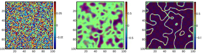
procedure, the sampling time in this example was chosen to be 5. The patterns of the system output at different times are plotted in Figure (2).

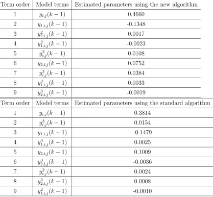
The new identification procedure proposed in Section 3.2 was performed with N = 3600 data randomly sampled from the space and time domain. The traditional CML identification algorithm [8] [9] was applied to provide a comparison with the new methods introduced above. The identified model terms and the corresponding coefficients are given in Table(1), where the terms y1,i,j(k−1) and y2,i,j(k−1) represent the combined output variables

of the neighbouring sites around the lattice (i, j), which are defined below to ensure a symmetric topology of coupling variables.

y1,i,j(k) = yi−1,j(k) +yi+1,j(k) +yi,j−1(k) +yi,j+1(k) (28)

0 10 20 30 40 50 60 70 80 −0.2 0 0.2 0.4 0.6 0.8 1 1.2

10 20 30 40 50 60 70 80 −0.2 0 0.2 0.4 0.6 0.8 1 1.2

Figure 1: Correlation functions φyy(τ) (left) and φy2_y2(τ) (right) from (10)

calculated fromNs = 1000 random data samples of the checkerboard patterns

in Example 1. It can be seen that the minimum time value isτm =τy2 ≈64.

20 40 60 80 100 20 40 60 80 100 −0.05 0 0.05

20 40 60 80 100 20 40 60 80 100 −1 −0.5 0 0.5 1

20 40 60 80 100 20 40 60 80 100 −1 −0.5 0 0.5 1

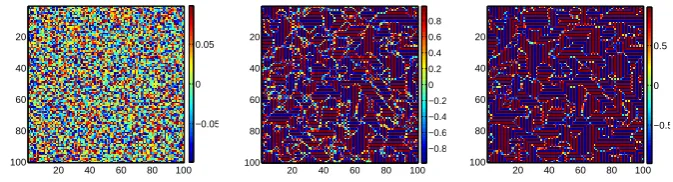
Figure 2: Snap shots of the CNN system simulation output for the checker-board patterns at the times k= 1,20,40 for Example 1, .

20 40 60 80 100 20 40 60 80 100 −0.05 0 0.05

20 40 60 80 100 20 40 60 80 100 −0.5 0 0.5

20 40 60 80 100 20 40 60 80 100 −0.5 0 0.5

Figure 3: Snap shots of the model predicted output of the identified model using the new algorithm at the times k = 1,20,40 for Example 1.

20 40 60 80 100 20

40

60

80

100

−0.05 0 0.05

20 40 60 80 100 20

40

60

80

100

−0.8 −0.6 −0.4 −0.2 0 0.2 0.4 0.6 0.8

20 40 60 80 100 20

40

60

80

100

−0.5 0 0.5

Figure 4: Snap shots of the model predicted output of the identified model using the standard algorithm at the times k = 1,20,40 for Example 1.

(3) that using the new identification algorithm, the dynamics of the original CNN patterns are well approximated by the identified CML model at every time step. However, as can be seen from the simulation results of the model identified using the standard CML method, the model predicted output at time t = 20 is quite different from the system output at that time.

4.2

Example 2: Stripe Patterns

Consider the CNN model with the A-template for the stripe patterns.

A=





−0.2 0 ₋0.2 0 0.8 0

−0.2 0 ₋0.2



 (30)

The initial state xi,j(0) for the stripe patterns was randomly distributed

between ₋0.1 and 0.1. Zero-flux boundary conditions were chosen. The above CNN model was numerically simulated with a time step ∆k = 0.1 over the space domain 100_×100.

The correlation based tests of the original data were applied to determine an appropriate sampling interval for the identification data. According to the simulation results in Figure (5) and the empirical selection method, the sampling time T can be chosen between τm/10 = 44/10 = 4.4 and τm/20 =

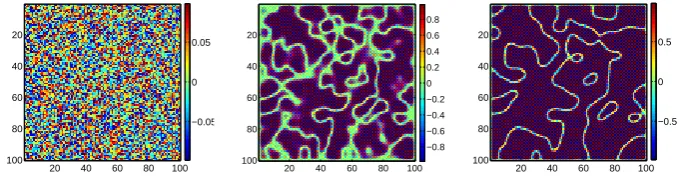
44/20 = 2.2. Here, the sample time for the identification data was chosen to be 3. Figure (6) shows snap shots of the system output at different times.

Table 1: Terms and parameters of the identified CML models for the checker-board pattern in Example 1

Term order Model terms Estimated parameters using the new algorithm

1 yi,j(k−1) 0.4660

2 y1,i,j(k−1) -0.1348

3 y2

2,i,j(k−1) 0.0017

4 y2

1,i,j(k−1) -0.0023

5 y2

i,j(k−1) 0.0108

6 y2,i,j(k−1) 0.0752

7 y3

i,j(k−1) 0.0384

8 y3

1,i,j(k−1) 0.0033

9 y3

2,i,j(k−1) -0.0019

Term order Model terms Estimated parameters using the standard algorithm

1 yi,j(k−1) 0.3814

2 y3

i,j(k−1) 0.0154

3 y1,i,j(k−1) -0.1479

4 y3

1,i,j(k−1) 0.0025

5 y2,i,j(k−1) 0.1009

6 y3

2,i,j(k−1) -0.0036

7 y2

i,j(k−1) 0.0024

8 y2

2,i,j(k−1) 0.0008

9 y2

1,i,j(k−1) -0.0010

10 20 30 40 50 −0.2 0 0.2 0.4 0.6 0.8 1 1.2

10 20 30 40 50 −0.2 0 0.2 0.4 0.6 0.8 1 1.2

Figure 5: Correlation functions φyy(τ) (left) and φy2_y2(τ) (right) from (10)

calculated from Ns = 1000 random data samples of the stripe patterns in

Example 2. It can be seen that the minimum time value is τm =τy2 ≈44.

20 40 60 80 100 20 40 60 80 100 −0.05 0 0.05

20 40 60 80 100 20 40 60 80 100 −1 −0.5 0 0.5 1

20 40 60 80 100 20 40 60 80 100 −1 −0.5 0 0.5 1

Figure 6: Snap shots of the CNN system simulated output for the stripe patterns at the times k = 1,30,60 for Example 2.

20 40 60 80 100 20 40 60 80 100 −0.05 0 0.05

20 40 60 80 100 20 40 60 80 100 −0.5 0 0.5

20 40 60 80 100 20 40 60 80 100 −0.5 0 0.5

Figure 7: Snap shots of the model predicted output of the identified model using the new algorithm at the times k = 1,30,60 for Example 2.

4.3

Example 3: Squiggle Patterns

20 40 60 80 100 20 40 60 80 100 −0.05 0 0.05

20 40 60 80 100 20 40 60 80 100 −0.8 −0.6 −0.4 −0.2 0 0.2 0.4 0.6 0.8

20 40 60 80 100 20 40 60 80 100 −0.5 0 0.5

Figure 8: Snap shots of the model predicted output of the identified model using the standard algorithm at the times k = 1,30,60 for Example 2.

dimensional space. A=      

−0.25 ₋1.0 ₋1.5 ₋1.0 ₋0.25

−1.0 2.5 7.0 2.5 ₋1.0

−1.5 7.0 ₋23.25 7.0 ₋1.5

−1.0 2.5 7.0 2.5 ₋1.0

−0.25 ₋1.0 ₋1.5 ₋1.0 ₋0.25

      (31)

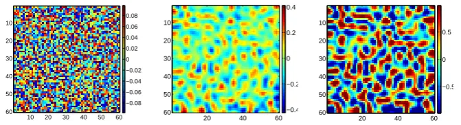
In this example, the radius of the coupling neighborhood was set to be 2. The random initial statexi,j(0) for the squiggle patterns was uniformly distributed

between₋0.1 and 0.1. Zero-flux boundary conditions were chosen. The CNN model with the above settings was numerically simulated with a time step ∆k = 0.1 over the space domain 60_×60.

Initially, the correlation based tests were applied to determine a sampling interval for the identification data. According to the simulation results in Figure (9), the sampling time T can be chosen between τm/10 = 160/10 =

16 and τm/20 = 160/20 = 8. In this example, the sample time for the

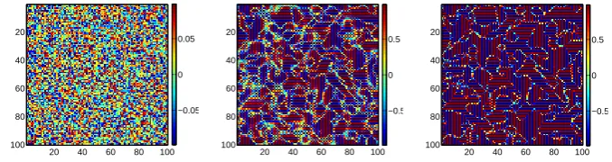
identification data was chosen to be 10. Figure (10) shows some snap shots of the system output of the squiggle patterns at different times.

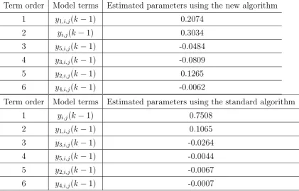
Two CML models were identified using both the new proposed algorithm and the standard algorithm. Table (3) gives the identified results from the two algorithms. The terms y1,i,j(k − 1) and y2,i,j(k −1) denote the same

combined variables as defined in the first example (28). Other terms in Table (3) are defined as follows

y3,i,j(k) = yi,j−2(k) +yi,j+2(k) +yi−2,j(k) +yi+2,j(k)

y4,i,j(k) = yi−1,j−2(k) +yi−1,j+2(k) +yi+1,j−2(k) +

yi+1,j+2(k) +yi−2,j−1(k) +yi−2,j+1(k) +yi+2,j−1(k) +yi+2,j+1(k)

Table 2: Terms and parameters of the identified CML models for the stripe pattern formation in Example 2

Term order Model terms Estimated parameters using the new algorithm

1 yi,j(k−1) 0.9239

2 y3

1,i,j(k−1) -0.0015

3 y2

1,i,j(k−1) -0.0018

4 y1,i,j(k−1) 0.0039

5 y2

2,i,j(k−1) 0.0001

6 y2

i,j(k−1) -0.0010

7 y2,i,j(k−1) -0.0711

8 y3

1,i,j(k−1) -0.0529

9 y3

2,i,j(k−1) 0.0024

Term order Model terms Estimated parameters using the standard algorithm

1 yi,j(k−1) 0.9729

2 y3

i,j(k−1) -0.1123

3 y2,i,j(k−1) -0.0711

4 y3

2,i,j(k−1) 0.0023

5 y2

i,j(k−1) -0.0030

6 y3

1,i,j(k−1) -0.0044

7 y2

2,i,j(k−1) 0.0002

8 y1,i,j(k−1) 0.0023

9 y2

1,i,j(k−1) -0.0014

50 100 150 200 −0.2 0 0.2 0.4 0.6 0.8 1 1.2

50 100 150 200 −0.2 0 0.2 0.4 0.6 0.8 1 1.2

Figure 9: Correlation functions φyy(τ) (left) and φy2_y2(τ) (right) form (10)

calculated from Ns = 1000 random data samples of the squiggle patterns in

Example 3. It can be seen that the minimum time value is τm =τy2 ≈44.

10 20 30 40 50 60 10 20 30 40 50 60 −0.08 −0.06 −0.04 −0.02 0 0.02 0.04 0.06 0.08

20 40 60 10 20 30 40 50 60 −0.2 −0.1 0 0.1 0.2

20 40 60 10 20 30 40 50 60 −0.8 −0.6 −0.4 −0.2 0 0.2 0.4 0.6 0.8

Figure 10: Snap shots of the CNN system simulation output of the squiggle patterns at the times k = 1,12,24 for Example 3.

10 20 30 40 50 60 10 20 30 40 50 60 −0.08 −0.06 −0.04 −0.02 0 0.02 0.04 0.06 0.08

20 40 60 10 20 30 40 50 60 −0.4 −0.2 0 0.2 0.4

20 40 60 10 20 30 40 50 60 −0.5 0 0.5

Figure 11: Snap shots of the model predicted output of the identified model using the new algorithm at the times k = 1,12,24 for Example 3.

5

Conclusions

10 20 30 40 50 60 10

20 30 40 50 60

−0.08 −0.06 −0.04 −0.02 0 0.02 0.04 0.06 0.08

20 40 60 10

20

30

40

50

60 −0.4

−0.2 0 0.2 0.4

20 40 60 10

20

30

40

50

60

−0.5 0 0.5

Figure 12: Snap shots of the model predicted output of the identified model using the standard algorithm at the times k = 1,12,24 for Example 3.

Table 3: Terms and parameters of the identified CML models for the squiggle pattern formation in Example 3

Term order Model terms Estimated parameters using the new algorithm

1 y1,i,j(k−1) 0.2074

2 yi,j(k−1) 0.3034

3 y5,i,j(k−1) -0.0484

4 y3,i,j(k−1) -0.0809

5 y2,i,j(k−1) 0.1265

6 y4,i,j(k−1) -0.0062

Term order Model terms Estimated parameters using the standard algorithm

1 yi,j(k−1) 0.7508

2 y1,i,j(k−1) 0.1065

3 y3,i,j(k−1) -0.0264

4 y5,i,j(k−1) -0.0044

5 y2,i,j(k−1) -0.0067

6 y4,i,j(k−1) -0.0007

dynamics of the CNN patterns over the long term.

6

Acknowledgements

The authors gratefully acknowledge that this work was supported by EP-SRC(UK).

References

[1] H. D. I. Abarbanel, R. Brown, and J. B. Kadtke, Prediction in chaotic nonlinear systems: Methods for time series with broadband fourier spec-tra, Phys. Rev. A41 (1990), 1782–1807.

[2] P. Arena, S. Baglio, L. Fortuna, and G. Manganaro, Self-organization in a two-layer cnn, IEEE Trans. Circuits Sys. I 42 (1998), 157–162.

[3] R. A. Barrio, C. Varea, J. L. Aragon, and P. K. Maini, A two-dimensional numerical study of spatial pattern formation in interacting turing systems, Bull. Math. Bio.61 (1999), 483–505.

[4] S. A. Billings and L. A. Aguirre, Effects of the sampling time of the dynamics and identification of nonlinear models, Int. J. Bifurcation and Chaos 5 (1995), 1541–1556.

[5] S. A. Billings, S. Chen, and M. J. Kronenberg, Identification of mimo non-linear systems using a forward regression orthogonal estimator, Int. J. Control 49 (1988), 2157–2189.

[6] S. A. Billings and Q. H. Tao, Model validity tests for non-linear signal processing applications, Int. J. Control 54 (1991), 157–194.

[7] L. O. Chua,Cnn: A paradigm for complexity, World Scientific Series on Nonlinear science E, 1998.

[8] D. Coca and S. A. Billings, Identification of coupled map lattice models of complex spatiotemporal patterns, Phys. Lett. A 287 (2001), 65–73.

[9] , Identification of finite dimensional models of infinite dimen-sional dynamical systems, Automatica 38 (2003), 1851–1856.

[11] P. Gray and S. K. Scott, Autocatalytic reactions in the isothermal, con-tinuous stirred tank reactor - isolas and other forms of multistability, Chem. Eng. Sci 38 (1983), 29–43.

[12] L. Z. Guo and S. A. Billings,Identification of coupled map lattice models of stochastic spatio-temporal dynamics using wavelets, Dynamical Sys-tem 19 (2004), 265–278.

[13] M. Itoh and L. O. Chua,Image processing and self-organizing cnn, Inter. J. Bifurcation and Chaos 15 (2005), 2939–2958.

[14] K. Kaneko, Spatiotemporal intermittency in coupled map lattices, Prog. Theor. Phys. 74 (1985), 1033–1044.

[15] , Turbulence in coupled map lattices, Physica D 18 (1986), 475– 476.

[16] ,Pattern dynamics in spatiotemporal chaos pattern selection, dif-fusion of defect and pattern competition intermittency, Physica D 34

(1989), 1–41.

[17] K. J. Lee, W. D. McCormick, Q. Ouyang, and H. L. Swinney, Pattern formation by interacting chemical fronts, Science 16 (1993), 192–194.

[18] J. L. Maron and S. Harrison, Spatial pattern formation in an insect host-parasitoid system, Science 278 (1997), 1619–1621.

[19] H. Meinhardt, The algorithm beauty of sea shells, Springer-Verlag, 1995.

[20] J. D. Murray, Mathematical biology, Springer-Verlag, 1989.

[21] Q. Ouyang and H. L. Swinney,Transition from a uniform state to hexag-onal and striped turing patterns, Nature352 (1991), 610–612.

[22] Y. Pan and S. A. Billings, The identification of complex spatiotemporal patterns using coupled map lattice models, Submitted for publication.