Data pruning

(1)

Thesis by

Anelia Angelova

In Partial Fulﬁllment of the Requirements

for the Degree of

Master of Science

California Institute of Technology

Pasadena,California

2004

(2)

c

2004

Anelia Angelova

(3)

Acknowledgements

I would like to thank my advisers Professor Pietro Perona and Professor Yaser

Abu-Mostafa for their help and support. This work would not have been possible without

them.

I would also like to thank my colleagues from the Vision Group and Learning

Systems Group at Caltech.

This work is supported by the National Science Foundation Research Center for

Neuromorphic Systems Engineering.

(4)

Abstract

Could a training example be detrimental to learning? Contrary to the common belief

that more training data is needed for better generalization,we show that the learning

algorithm might be better oﬀ when some training examples are discarded. In other

words,the quality of the examples matters.

We explore a general approach to identify examples that are troublesome for

learning with a given model and exclude them from the training set in order to

achieve better generalization. We term this process ’data pruning’. The method is

targeted as a pre-learning step in order to obtain better data to train on.

The approach consists in creating multiple semi-independent learners from the

dataset each of which is inﬂuenced diﬀerently by individual examples. The multiple

learners’ opinions about which example is diﬃcult are arbitrated by an inference

mechanism. Although,without guarantees of optimality,data pruning is shown to

decrease the generalization error in experiments on real-life data. It is not assumed

that the data or the noise can be modeled or that additional training examples are

available.

Data pruning is applied for obtaining visual category data with little supervision.

In this setting the object data is contaminated with non-object examples. We show

that a mechanism for pruning noisy datasets prior to learning can be very successful

especially in the presence of large amount of contamination or when the algorithm is

sensitive to noise.

Our experiments demonstrate that data pruning can be worth while even if the

algorithm has regularization capabilities or mechanisms to cope with noise and has a

(5)

List of Figures

3.1 Average test errors when training on subsets of the data with increasing

diﬃculty of examples . . . 21

3.2 Training on subsets of the data may provide for decreasing the general-ization error . . . 23

3.3 Training on subsets of the data may provide for decreasing the general-ization error. Single run on the training data . . . 24

3.4 Inherent model complexity is increased by adding more difficult examples 26 3.5 Algorithms may share boundaries and therefore the difficult examples . 29 3.6 Definition of a difficult example depends on the model . . . 30

3.7 Data pruning results . . . 36

3.8 Data pruning results for UCI datasets . . . 37

4.1 Training data for face category . . . 41

4.2 Dictionary of ﬁlters . . . 43

4.3 Masks selecting sub-regions of the object . . . 43

4.4 Sub-regions for training multiple independent learners for face category 44 4.5 Data pruning results for contaminated face data . . . 46

4.6 Data pruning results for contaminated face data. Scatter plots . . . 47

4.7 Comparison between diﬀerent pruning mechanisms and diﬀerent basic learning algorithms . . . 48

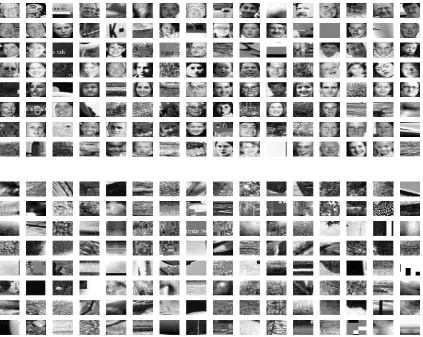
4.8 Examples selected for elimination by bootstrapped learners . . . 49

4.9 Examples selected for elimination by region learners . . . 50

(9)

List of Tables

4.1 Average test error for learning on pruned and full face data,SVM

algo-rithm. Pruning based on bootstrapped learners . . . 47

4.2 Statistics on the identiﬁed wrongly labeled examples. Bootstrapped

learners. . . 51

(10)

Chapter 1 Introduction

1.1 Learning and Generalization

A learning task can be deﬁned in the following way: given a set of training examples

S ={(x₁, y₁), ...,(xN, yN)} which supposedly come from an unknown target function

f : X → {−1; +1} , yi = f(xi), i = 1. . . , N ﬁnd a function g, g : X → {−1; +1},

g ∈G={g}which agrees with the target functionf as well as possible. The learning

model G is a predeﬁned set of hypotheses from which the target function is selected.

The purpose of learning machines is to be able to classify correctly unseen

exam-ples,not only the training ones. In other words,to generalize well rather than simply

memorize the training data. If the learning algorithm performs well on the training

data but poorly on unseen data,overﬁtting is said to occur.

1.2 Diﬃcult examples and outliers

In real-life problems it is possible that the training data is contaminated by noise,

meaning yi = f(xi) is not satisﬁed for all of the examples. Those wrongly labeled

examples would be problematic for the learning process. An important task of a

learning algorithm is to be robust to noisy or mislabeled examples.

Troublesome examples may also be ones which are diﬃcult in a sense that in order

to learn them the algorithm would be in contradiction with other training examples,

(11)

these hard examples may lead to the algorithm being unable to generalize well or

overﬁt.

In the presence of troublesome examples,the learning machine has to face a very

diﬃcult task: it has to learn an unknown function using a ﬁnite number of examples

considering that some of the examples may be misleading or diﬃcult in other ways.

We would like to explore if it is possible to ﬁnd mechanisms to detect and eliminate

examples hard for learning and improve the generalization performance by doing so.

1.3 Data pruning overview

1.3.1 What is data pruning?

Suppose we are given a set of training examples and a selected learning model. The

task is to identify if there are examples in the training set such that by eliminating

them one may improve generalization performance.

Many methods deal with noisy examples by querying for more

data,accommo-dating the examples by reweighting or decreasing their inﬂuence by regularizing the

solution. We will study methods that fully eliminate those ’bad’ examples from

train-ing or,in other words,prune the traintrain-ing data.

The most challenging problem is how to deﬁne for a particular training data and

selected model which examples are worth removing so that to improve generalization

ability of the learner.

1.3.2 Overview of data pruning method

Our approach consists in learning diverse classiﬁers (learners) by randomizing the

training set and then combining their output to decide on diﬃcult examples. We use

a bootstrapping method to select various semi-independent learners.

Each of the new learners would be capable of classifying the data comparably to

the learner on the full-sized training set. However,each one is trained on a diﬀerent

(12)

semi-independent opinions with respect to the troublesome examples. Our intuition is that

most of the learners would agree on non-diﬃcult examples. Furthermore,examples

which are forcing poor generalization performance would not inﬂuence all the learners.

So,combining the output of all the learners may help identify the troublesome training

examples. The classiﬁers’ opinions are combined using Bayesian reasoning to receive

a ﬁnal decision of whether an example has to be eliminated.

We apply the data pruning method to learn to recognize face category from very

noisy datasets. As the target is visual category,multiple semi-independent learners

can be received by training on slightly overlapping regions containing parts of the

(13)

Chapter 2 Identifying noisy examples

In this chapter we give a notion of which example is diﬃcult and show various ways

to deal with outliers,noisy or diﬃcult examples in diﬀerent areas of learning from

examples.

2.1 Introduction

2.1.1 What is a diﬃcult example?

Formal deﬁnition of diﬃcult examples is hard to give. Below we give informal

defini-tion of outliers or difficult examples. Difficult examples are those which obstruct the

learning process or mislead the learning algorithm or those which are impossible to

reconcile with the rest of the examples.

Deﬁning diﬃcult example cannot be done without the learning model or the

gen-erating distribution.

The reliability of an observation is dependent on the other

observations,i.e.,defin-ing difficult example should be done in the context of the remainobservations,i.e.,defin-ing data. The

rela-tive number of outliers with the same ’weirdness’ should be small,i.e.,the particular

properties of an outlier are not supported by many other examples.

Quite often in statistics the method advocated is through visual examination of

the data or the residuals after ﬁtting a particular model. Further elimination of values

(14)

of a diﬃcult example very subjective and prone to errors due to misspeciﬁed model.

As a summary,an outlier is discordant with the remaining data and with respect

to the model.

We would use interchangeably the terms outliers,diﬃcult,adversary,noisy and

troublesome example. Alternative names common in the literature are discordant

observations,contaminants,surprising values.

2.1.2 How to deal with outliers?

Deﬁning what a diﬃcult example is and how to cope with it are two interconnected

problems.

Diﬀerent approaches have been taken trying to be robust to outliers: discard them,

give diﬀerent weights to more inﬂuential examples,average out multiple observations

so that to diminish the poor inﬂuence of outliers in some models or accommodate them

in a redesigned model. Discarding examples is suitable in the case of inherently wrong

observations. It can improve the accuracy of the mean. Reweighting is suggested

for heavy tailed distributions,for example,give weights according to the standard

deviation. Averaging out observations would reduce the variance.

In this work we will eliminate the outlying examples altogether.

2.1.3 Why deﬁning outliers is diﬃcult?

Outliers and diﬃcult examples may come from various sources and may be realizations

of diﬀerent phenomena. So,assuming a particular model for the noise might not be

always appropriate.

Diﬃcult examples may be noisy e.g. coming from diﬀerent than the assumed

distribution,or may be the result of wrong measurements.

In statistics an outlier can be deﬁned from the generating distribution. Given the

distribution,an outlier is a value which deviates ’too much’. This,in the ﬁrst place,

is not a clear-cut deﬁnition because it is not known what deviations are tolerable.

(15)

one.

An example may be a result of natural variation and the model should be able to

handle those without discarding them as outliers.

Furthermore,the learning algorithm may react in diﬀerent ways to the presence

of outliers: some algorithms might be able to learn in the presence of noise,others

would be more severely inﬂuenced by adversary examples,resulting in poorer decision

boundary and worse generalization performance.

2.1.4 Motivation: Why study outliers?

The outliers themselves can be a main interest for practical purposes such as detection

of anomalies,interesting observations,etc.

The other side of the story is that outliers may just be measurements which are

wrong and subsequently would force the incorrect model parameters to be estimated

or the function selected may not generalize well because of overﬁtting with respect

to those diﬃcult examples. In those cases the troublesome examples are again of

interest but to be considered for elimination.

An example which is too inﬂuential in the model can change the estimation of

the model. For example,outlying observations can result in a wrong estimate of the

mean of the population.

Moreover,in data analysis,identifying and studying outliers provides important

information as to how adequate the current model is and may suggest a revision of

the model and its assumptions.

As we have discussed so far,deﬁning a diﬃcult example is quite subjective. A

statistically objective method to identify and deal with outliers is still a topic of

research. In the following sections we review several methods to identify and cope

(16)

2.2 Robust statistics

Robust statistics is preoccupied with how to identify outliers or noisy observations,

eliminate their inﬂuence or fully discard them [5],[21]. We give some examples of

how robust estimation can be done.

2.2.1 Accommodating outliers

One straightforward approach is to reweight the observations according to their

in-ﬂuence or the conﬁdence we have in them and re-estimate the model parameters.

Alternative one is to use more robust cost functions. For example,the least

squares objective function_i(Xi−M)2 ,whereM denotes the ﬁtted model for linear

regression,is notorious for being very sensitive to outliers. Huber [21] suggested to

use other cost functions_iρ(Xi−M) which are more robust to outlying observations,

for example ρ(t) =|t| [5].

Another approach is to modify the model so that it takes into consideration

out-lying observations.

2.2.2 Eliminating outliers

Various statistical tests have been created for particular cases of identifying one or

two outlying observations. Examples are removed one at a time and the model is

re-estimated. Students’ tests are used to decide if an observation is deviating too

much when not included in the estimation [43].

Robust estimation by examining residuals and removing examples can be done

for linear models with normal distributed noise Y = Xβ+e, var(e) = σ2I,where

X is a set of data points, Y are the responses and a linear model needs to be ﬁt to

those points so that to minimize the least-squares error of the ﬁt [43]. β contains

the parameters of the linear model and e is a vector of residual errors. The

least-squares estimate ˆY is computed as follows ˆY=X(XTX)−1XTY=HYˆ where Hˆ is

(17)

be removed. The inﬂuence of example Xi is determined by hii in the ’hat’ matrix.

Details are given below.

The residuals are deﬁned as e=Y−Yˆ = [I−Hˆ]Y. The residual of an example

satisﬁes var(ei) = σ2(1−hii),i.e.,values of hii close to 0 mean that the example

would have a large deviation of the error estimation and suggests that it might be an

outlier. However,caution should be taken because this might not always be so: the

hii value should be considered in the context of the other hij in the ’hat’ matrix [43].

Another way to estimate the inﬂuence of examples is by perturbing the data and

examining again the residuals. Examples which result in major changes of the model

are considered inﬂuential [43].

Many estimators are created particularly to improve the robustness of the mean

or other statistics of the data but we would not examine them here.

The practice in robust statistics is to identify outliers for further investigation.

The actual elimination is done after human supervision. In this work we explore an

approach which would automatically identify and eliminate outlying examples.

Generally,in statistics,it is recommended that the samples be ’routinely

sub-jected’ to outlier detection procedures before estimating the model. This diagnostic

might help to validate the adequacy of the model,to guide the subsequent data

anal-ysis,to take into consideration examples which might need to be further investigated,

rejected or accommodated by the model [5].

2.2.3 RANSAC

The RANSAC (RANdom SAmple Consensus) algorithm [16] is used to learn model

parameters in the presence of large number of outliers. It randomly samples minimal

subsets of the data to estimate the model parameters and selects the model with

maximum agreement among the samples.

It is assumed that the target model is known and a ﬁxed number of data points

(18)

algorithm proceeds by selecting multiple times (T trials) a random subset of m data

points,estimate the model parameters and rate the selected model correspondent to

how much it complies with the rest of the data. Out of the many attempts to ﬁt a

model the one which ﬁts the whole data best is selected. It relies on the fact that

in data containing a large amount of outliers (50% or more) the model parameters

selected using the outliers would be inconsistent with each other,while the correct

model parameters would be consistent throughout many trials. So,in order to

esti-mate them with high conﬁdence a suﬃcient number of trials is needed.

RANSAC is often used in vision applications for example to ﬁt geometric

primi-tives e.g. a line or a circle to a set of noisy points,to ﬁnd point correspondences,or

to ﬁnd a matrix for a transformation which best explains the evidence (usually very

noisy). A trivial example of using RANSAC is as follows: if we need to ﬁnd a circle

which is consistent with a lot of noisy points,three points are suﬃcient to determine

the circle center at each trial,the most frequent center of circles is selected as the

best model.

The RANSAC algorithm requires the target model to be known and the number

of examples to estimate it uniquely should be small. In our task of data pruning

we are uncertain about both model complexity,and subset of data needed for

esti-mating learning. There is a large degree of freedom introduced by the model and its

complexity being unknown.

2.3 Regularization methods

Regularization methods are created to deal with problems which are ill-posed,namely,

the solution may not exist,is not unique or is unstable to small perturbations in the

initial data [39]. Generally,regularization methods apply penalty or restriction on the

class of admissible solutions so that the problem becomes a well-posed one. There

is a large body of work on regularization with applications in solving diﬀerential

equations,inverse problems,linear integral equations,etc.

(19)

Suppose the problem consists in minimizing a functional R(X) depending on the

training data. Regularization methods suggest to minimize R(X) +λΩ(X) instead,

where Ω(X) is a stabilizing functional or penalty. It may express desired properties

of the solution,for example,we can penalize for a function with large derivatives to

prefer a smoother (less oscillatory) function. The new target function is a trade-oﬀ,

controlled by the coeﬃcient λ,between ﬁtting the data and using too complex a

function.

There are other forms of regularization. Below,we discuss some of them. Without

trying to encompass all,we consider only cases which are relevant to learning and

more speciﬁcally to dealing with noisy examples or outliers.

2.3.1 Regularization with penalties

The most popular form of regularization is the weight decay for Neural Networks,

where the penalty is over the sum of squares of all parameters in the network,namely

its weights [6]. The regularizing functional penalizes large sum of weights in the

network which may lead to overly complex discrimination function: Ω = 1₂_iw2_i.

A heuristic with similar purposes is early stopping,in which smaller number of

iterations of the learning process (epochs) is preferred. It has a regularization eﬀect

because more epochs are more likely to create more complex network and therefore

overﬁt the data [6].

Theoretical justiﬁcation for preferring smaller sum of weights with weight decay

or early stopping in Neural Networks was given by Bartlett [3]. He showed that the

generalization ability of the Neural Network depends on the sum of weights of the

network. Thus networks with larger weights may be of large complexity,which would

increase the generalization error.

2.3.2 Introducing slack variables

We demonstrate the method of using slack variables for regularization with the so

(20)

of SVM classiﬁcation for linearly separable data is to ﬁnd a hyperplane y=w,x +b

which achieves maximum margin measured as _w1₂,for both classes. The following

problem needs to be solved:

min 1₂w2 subj.to

yi(w,xi +b)≥1 i= 1, . . . , N

To cope with linear nonseparability,the kernel trick is applied and the dataset

is transformed to high dimensional space [36]. Still,even in high dimensional space,

the data may not be perfectly separable and some form of regularization is needed.

Cortes and Vapnik [14] suggest to introduce slack variables which allow some data

points to violate the decision boundary. This method has proved to be very successful

in practice.

min 1₂w2−CN_i₌₁ξi subj.to

yi(w,xi +b)≥1−ξi, ξi ≥0 i= 1, . . . , N

2.3.3 Case study: Regularizing AdaBoost

Boosting algorithms and in particular AdaBoost [18] combine weak learners,learners

performing slightly better than random guessing,into a strong one. The crucial idea

of boosting is to give larger weights to examples wrong with respect to the current

weak learner. Thus examples which are generally diﬃcult would get consistently

larger weights.

Boosting methods are of particular interest to us,because their internal mechanism

is to overemphasize diﬃcult examples - a strategy opposite to outlier elimination or

de-emphasizing. Yet,in noisy cases,this strategy of AdaBoost has shown in experiments

to be suboptimal. Therefore some sort of regularization is needed.

Jiang [22] supported theoretically the claim by demonstrating that ’boosting

for-ever’ leads to suboptimal solutions and that a regularized version of boosting would

(21)

2.3.3.1 Applying penalties

The standard way of applying penalty to the cost function to be minimized can be

straightforwardly applied to AdaBoost.

Mason et al. [29] presented an interpretation of boosting methods as a gradient

descent over some cost function. By minimizing the cost function at each iteration,

the gradient descent algorithm selects a best hypothesis and a coeﬃcient,which is

equivalent to modifying the weights over the examples in order to select the next best

hypothesis in the original boosting algorithm.

AdaBoost algorithm can be exactly retrieved from this framework with the

expo-nential cost function over the margin of an example,deﬁned asγ(xi) =yi

_T

t=1αtgt(xi)

G=

N

i=1

e−yiT_t₌₁αtgt(xi)

where {xi, yi}Ni=1 is the training set of N examples and T is the number of

itera-tions.

R¨atsch et al. [33],[34] proposed to regularize AdaBoost by modifying the cost

func-tion at each iterafunc-tion through adding penalty for diﬃcult examples. Their criterion

for a diﬃcult example is the average weight of an example of all the iterations up

to the current one. The cost function to be minimized at iteration t₀ by AdaBoost

becomes:

Gt0 ₌

N

i=1

e−yi(t_t0₌₁αtgt(xi))−Cµ(x_i)

whereµ(xi) = (

_t₀

t=1αtwt(xi))2 andwt(xi) is the weight of an example at iteration

t and C is a ﬁxed constant. The rationale behind this type of regularization is that

examples which are hard would tend to be over-emphasized and therefore would have

large sum of weights throughout previous iterations. Therefore,the algorithm might

(22)

2.3.3.2 Introducing slack variables

Another way to regularize AdaBoost solution is to introduce slack variables [33],[34],

as with SVM. An approximation of AdaBoost,called LP-AdaBoost [20],is used. In

LP-AdaBoost the hypotheses are selected using AdaBoost and then linear

program-ming is used to ﬁnd best combining coeﬃcients in order to achieve maximum margin.

Grove and Schuurmans [20] showed experimentally that maximizing the minimum

margin gives a suboptimal solutions especially in noisy cases. Slack variables are

introduced in the optimization problem so that to allow the algorithm to give up on

some noisy examples (to allow for some diﬃcult examples to violate the maximum

margin condition). The formulation of regularized version of LP-AdaBoost is:

max γ−CN_i₌₁ξi subj.to

yi

T

t=1αtgt(xi)≥γ−ξi, ξi ≥0, i= 1, . . . , N

αt≥0,

_T

t=1αt= 1, t= 1, . . . , T

where gt(x) are the hypotheses already found by AdaBoost and αt are the

coeﬃ-cients we are optimizing for and C is a ﬁxed regularization constant.

2.3.3.3 Modifying the cost function

Mason et. al. [28] suggest that a cost function of special type is used,so that not

to emphasize too much examples which might be noisy. AdaBoost cost function is

exponential,i.e.,it would give exponentially large weights to misclassiﬁed examples.

Instead they propose optimizing over a family of less steep cost functions.

Manipu-lating the cost function so that it penalizes more diﬃcult examples is again some sort

of regularization for a class of boosting techniques.

2.3.3.4 Removing examples

Regularization by removing examples for AdaBoost,termed ’example shaving’,has

been demonstrated by Merler et al. [30]. A level of diﬃculty of an example is

(23)

the entropy of the weight distribution throughout iterations for each example [11]. A

validation set is used to deﬁne which of the most diﬃcult examples to be removed [30].

The usefulness of regularizing AdaBoost has been demonstrated experimentally

in noisy datasets [28],[33],[34]. The need for regularizing AdaBoost has been

theo-retically explained in [22].

2.4 Learning with queries

2.4.1 Learning in the presence of classiﬁcation noise

Angluin and Laird [2] investigated learning in the presence of classiﬁcation noise in

the context of learning with queries. In the classiﬁcation noise scenario examples have

their labels ﬂipped with a certain probability β,but are otherwise not changed,i.e.,

they are assumed to come from the target distribution. They showed that if the noise

can be modeled as independent source then the amount of noise tolerated can be

very large but strictly less than 50%. For this setting they give a sample complexity

bounds for eﬀective learning in which the number of examples is polynomial in ₁₋1₂_β,

where β is the noise level. That is,considerably more examples are needed to learn

the concept if the level of noise is large. They proved that learning in the presence

of noise is possible but the search for an optimal hypothesis for general problems is

polynomially intractable with their approach. For some classes of concepts eﬃcient

algorithms exist which exploit the properties of the particular concept class.

2.4.2 Learning in the presence of malicious noise

Kearns and Li [23] consider an extension of learning with noise in which the noise is

not assumed to have nice properties and generally cannot be modeled. The adversary

creating the noise has ultimate powers such as changing examples’ labels,returning

examples from a wrong distribution,having access to the currently generated

(24)

learned examples. This model is called learning with malicious noise. For this model

signiﬁcantly smaller amounts of noise can be tolerated. The authors give hardness

results for learning of arbitrary concepts in this model as well as constructive learning

algorithms for learning particular concept classes.

2.4.3 Active learning

The objective of active learning is to select particularly informative examples in order

to speed up training [25],[13].

In some sense active learning is also preoccupied with excluding examples from

the dataset,but there,the redundant examples are the ones to be ignored. Smaller

number of data points and considerably less computational resources are required in

active learning than in the standard learning scenario to achieve the same

generaliza-tion performance [41]. The assumpgeneraliza-tion of active learning is that the training data is

not noisy.

2.5 Outliers in a probabilistic setting

Finding and eliminating outliers can be cast in a probabilistic setting. A generative

probabilistic models are assumed for the two classes’ distributions. An appropriate

outlier model is selected. A new hidden variable is introduced for an example being

an outlier (and therefore need to be eliminated or ignored) and the problem can be

solved with maximum likelihood approach and the EM [17].

Although the method is very powerful its disadvantages come from the strong

assumptions made,namely the models of data distributions and outliers should be

known. Apart from that,more parameters for the generatve models need to be

estimated,i.e.,more training data would be necessary,which might not always be

(25)

2.6 Data valuation

The methods described above introduce mechanisms to cope with noisy situations,

usually by imposing penalty,by de-emphasizing (reweighting) noisy examples. The

most common case is trying to ignore them by overpowering the presence of noisy

examples by using more correct ones. Data valuation method,proposed by

Nichol-son [32],advocates removing examples from the training data and demonstrates it is

useful on several classiﬁcation problems with noise.

Data valuation [32] consists in analyzing the training data prior to learning and

removing examples which might be adversary to learning. The examples are given a

ranking according to their agreement with the remaining data and examples which

disagree most are removed. Data valuation is created for the exhaustive learning

scenario.

2.6.1 Exhaustive learning

The exhaustive learning algorithm [37] returns hypotheses from the learning model

with a ﬁxed prior distribution. Thus any hypothesis in the support of the prior

dis-tribution can be selected. That is,no actual learning is performed on the data. Note

the distinction from the standard learning scenario where only hypotheses which

per-form well with respect to the training data (for example minimize the empirical risk)

are selected. The distribution over hypotheses in the learning model in exhaustive

learning is independent (agnostic) of the training data.

Although the analysis of [32] is done for the exhaustive learning scenario [37],we

consider the data valuation method as a predecessor to our work.

2.6.2 ρ

-criterion

A primary task in data elimination is to deﬁne which examples are diﬃcult for

learn-ing and therefore candidates for elimination. Nicholson [32] proposes a heuristic for

(26)

the overall error rate π in the exhaustive learning. As π is unknown it is

approxi-mated by the leave-one-out error,the error of the dataset excluding the example in

question.

ρ_x_i =corrg(ei(g), eSi(g))) =

Eg(ei(g)eSi(g))−Eg(ei(g))Eg(eSi(g)) V ar(ei(g))V ar(eSi(g))

(2.1)

wherecorr is correlation of the error of the examplexi,denoted byei(g),with the

error of the remaining set,denoted byeS_i(g),Si =S\xiandS ={(x1, y1), ...,(xN, yN)}

is the training set.

Furthermore,because the expected value of errors with respect to all hypotheses

inGcannot be computed analytically in most of the cases,(2.1) will be approximated

by randomly sampling hypotheses from the learning model.

Thus a ρ value (2.1) is assigned to each example showing how much it agrees

with the target function for this particular model. It gives information whether the

example is contradicting on average the rest of the examples with respect to all

possible hypotheses. The higher the correlation the more the example complies with

the remaining training set,i.e.,would not be expected to be troublesome in learning.

Examples with negative correlation ρ would be expected to be diﬃcult using this

learning model. In practice Nicholson [32] has shown thatρneeds to be selected close

to -1 in order to avoid deterioration in performance,which is probably due to the

approximations in calculating ρ.

The author demonstrated that in noisy datasets removing examples from the

(27)

Chapter 3 Data pruning

3.1 Introduction

In the previous chapter we have reviewed several learning methods which have

mech-anisms to cope with noisy examples. Some of them apply a common penalty for all

examples (regularization methods),others identify those examples which inﬂuence

the model too much and reweigh them,assuming that the model is known and ﬁxed

(robust statistics),others model the noise source as independent white noise [2] and

show that learning can be done,provided that suﬃcient examples are available.

Suc-cessful identiﬁcation of outliers can be done for models which are ﬁxed and have very

few parameters to estimate e.g. RANSAC [16]. In those cases a large amount of noise

can be tolerated.

In many real-life learning problems noise is often present,the number of examples

is insuﬃcient and the model and its complexity are not known a priori. Our goal is

to look into those more realistic settings.

We are interested in binary classiﬁcation tasks in which we are given a ﬁxed

training set and a desired model for classiﬁcation. In this setting we want to identify

examples which are troublesome for the learning process for this particular training

set and this particular model and which might potentially cause the model to overﬁt

and therefore deteriorate the generalization performance. We term data pruning the

process of eliminating examples which might be troublesome for learning.

(28)

the diﬃculties of solving it. We propose a way to identify and eliminate troublesome

examples and show experiments and promising results of data pruning on real-life

data.

In the next chapter we apply our method to the recognition of object categories

in which the training data is contaminated,namely,the data may have large amount

of wrongly labeled examples or examples which are otherwise diﬃcult for the model

at hand.

3.2 Problem formulation

Data pruning may be deﬁned as follows: given training data and a learning model,ﬁnd

if there are training examples for which the learning and generalization performance

would be improved after removing those examples. The problem as we deﬁne it is

quite diﬃcult to solve. Below,we examine the reasons why.

Eliminating the inﬂuence and detrimental eﬀects of outliers is still an active area

of research in statistics. The main challenges come from the diﬃculty of modeling

outliers because their sources may be variable. In our case we do not assume a model

of the noise.

We are considering a binary classiﬁcation problem which is ill-posed in the ﬁrst

place even without any noisy examples. This is because the training data is ﬁnite

and a small change in the data,for example adding or removing a few examples,can

change the decision boundary. Apart from that the solution is not unique as the most

appropriate model and model complexity are not speciﬁed [36].

Straightforward approaches to solve the problem are to sort the examples in

in-creasing level of diﬃculty,diﬃcult meaning closer to the decision boundary [11] or

level of disagreement [32] and eliminate sequentially most diﬃcult ones. An

indepen-dent test set is used to iindepen-dentify which examples to be removed [30]. Although using

validation set can be very useful,in this case we feel that using additional data to

decide which examples to prune gives an unfair advantage of the pruned method with

(29)

set in order to choose their best parameters but we feel we cannot allow the algorithm

to decide on pruning an example or not using extra validation set.

A lot of research has been done in using unlabeled data alongside with labeled.

The major conclusion being that using unlabeled data in addition to labeled is quite

useful and handy when labeling is expensive. Those depend on the assumption that

they have some reliably labeled data to start the learning and estimation from [8]. In

our formulation we have to identify the correctly labeled examples.

And last but not least,the powerful probabilistic models can be applied very

successfully to solve fully unsupervised problems modulo some technical problems

with local minima and amount of data needed to estimate the parameters correctly.

Those methods rely on the strong assumption that the data comes from a particular

distribution which can be modeled. If the assumption is correct Bayesian methods

would give the optimal solution. Nevertheless,we believe we cannot generally assume

we know and can model the sources that generated the data and want to use the

available training data in less requiring discriminative models.

3.3 The essence of data pruning problem

In this section we try to understand the problem of identifying troublesome examples

and removing them from the data. We would give examples to get intuition of the

problem at hand.

3.3.1 When is data pruning necessary?

We give characteristic examples of datasets with and without diﬃcult examples and

show where data pruning would be helpful. We show those characteristic behaviors

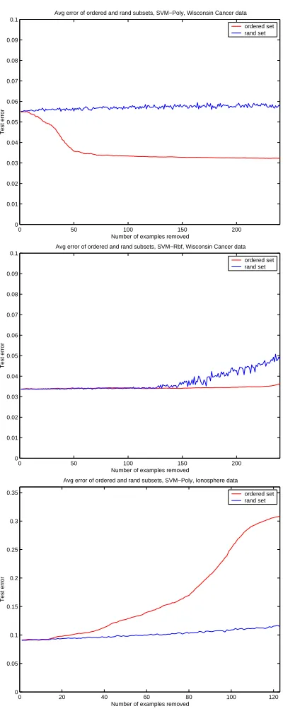
on real datasets,ﬁgure 3.1.

(1) There are examples adversary to learning present in the dataset,diﬃcult

examples can mislead the algorithm and it creates a poor boundary or overﬁts. The

(30)

0 50 100 150 200 0 0.01 0.02 0.03 0.04 0.05 0.06 0.07 0.08 0.09 0.1

Avg error of ordered and rand subsets, SVM−Poly, Wisconsin Cancer data

Number of examples removed

Test error

ordered set rand set

0 50 100 150 200

0 0.01 0.02 0.03 0.04 0.05 0.06 0.07 0.08 0.09 0.1

Avg error of ordered and rand subsets, SVM−Rbf, Wisconsin Cancer data

Test error

0 20 40 60 80 100 120

0 0.05 0.1 0.15 0.2 0.25 0.3 0.35

Avg error of ordered and rand subsets, SVM−Poly, Ionosphere data

Test error

[image:30.595.225.425.68.571.2]

(31)

(2) There are examples adversary to learning present in the dataset but the

al-gorithm has mechanisms to ignore noisy examples in its optimization (for example

SVM-SVC,Neural Networks). No matter that,the algorithm cannot always deal with

hard examples. In those cases adversary examples can lead to poorer generalization

performance,as in case (1).

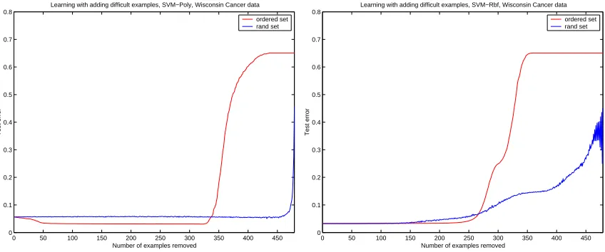
(3) There are no examples adversary to learning in the dataset. Adding more

diﬃcult examples improves the test error,the diﬃcult examples are actually useful

for forming the proper boundary.

The plots of ﬁgure 3.1 show the three characteristic examples on real-life data

from UCI Repository [7] in which data pruning may or may not be useful. We should

note that the model in (1) has regularization capabilities but still cannot deal with all

diﬃcult examples. Conversely,on the same training data,the model in (2) can deal

with diﬃcult examples,which suggests that diﬃcult examples are model dependent.

The ordering of examples used to generate these plots would be explained in the next

section.

The plots also give intuition that training on subsets of the data with

increas-ing diﬃculty gives a chance to improve the generalization performance compared to

training on the whole training data as is in case (1).

3.3.2 Beneﬁts of data pruning

In this section we show that,given a learning model and a dataset,it is possible that

the algorithm would perform better if training on a subset rather than on the whole

set. One example has already been given in the previous section. To do that we need

to search for good subsets of the data. Finding the best subset of examples to train

on would need exponential number of subsets to be considered. Instead,we suggest to

deﬁne a measure of diﬃculty of an example and train on nested subsets of examples

of increasing complexity,hoping that if there are examples which are troublesome

(32)

the generalization error.

We propose to use the margin of an example as a criterion for how diﬃcult it

is and order the examples in terms of margin. However,we do not know the exact

complexity of the model according to which to measure the margin of the examples.

So,we suggest to learn the model using various complexities: create nested classes

of increasing capacity as in Structural Risk Minimization (SRM) [40],measure the

margins of each example and average them with respect to all models to get a more

reliable margin estimate.

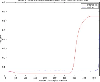
0 50 100 150 200 250 300 350 400 450 0

0.1 0.2 0.3 0.4 0.5 0.6 0.7 0.8

Learning with adding difficult examples, SVM−Poly, Wisconsin Cancer data

Test error

[image:32.595.157.493.257.533.2]

Figure 3.2: Training on subsets of the data of increasing complexity may provide for decreasing the generalization error. Learning algorithm is SVM. Wisconsin cancer data,0% noise.

This criterion is quite natural as the margin is a measure of conﬁdence in

classi-ﬁcation in an algorithm [35]. It is also a universal quantity because the margin of an

examples can be measured no matter what learning algorithm we use.

An interesting observation is that from this heuristic measure of diﬃculty we can

(33)

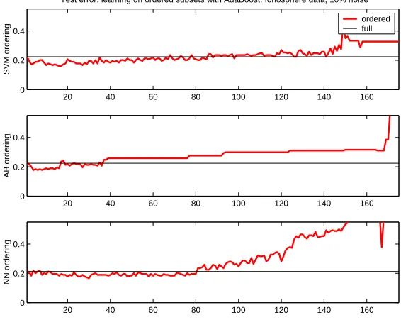
20 40 60 80 100 120 140 160 0

0.2 0.4

SVM ordering

Test error: learning on ordered subsets with AdaBoost. Ionosphere data, 10% noise

ordered full

20 40 60 80 100 120 140 160

0 0.2 0.4

AB ordering

20 40 60 80 100 120 140 160

0 0.2 0.4

NN ordering

50 100 150 200 250

0 0.1 0.2 0.3

SVM ordering

Test error: learning on ordered subsets with SVM. Wisc cancer data, 0% noise

ordered full

50 100 150 200 250

0 0.1 0.2 0.3

AB ordering

50 100 150 200 250

0 0.1 0.2 0.3

[image:33.595.182.465.79.313.2]

NN ordering

Figure 3.3: Training on subsets of the data may provide for decreasing the general-ization error. Each ﬁgure shows the test error for a single run of dataset ordered in terms of diﬃculty. Ordering criteria are computed using the average margin for SVM, AdaBoost and Neural Network models. Top: AdaBoost learning model,Ionosphere data,10% noise,Bottom: SVM learning model,Wisconsin cancer data,0% noise.

in AdaBoost. The authors used the criterion to impose regularization penalty.

(34)

error using such naive and heuristic way to order examples in terms of diﬃculty,

ﬁgures 3.2,3.3. The plots are generated by multiple randomized runs,so we can see

an estimate of the out-of-sample error,ﬁgure 3.2,and for only a single run ﬁgure 3.3 to

demonstrate that this phenomenon can be observed for a particular training dataset.

We note that this is not data pruning yet. We merely demonstrate that data

pruning has potential for some datasets which contain diﬃcult examples. Note that

there are datasets in which none of the examples are useless or harmful,as shown on

ﬁgure 3.1.

In this paragraph we have seen that it is possible to improve the generalization

error if training on a (suitably chosen) subset of the training data,for the sole reason

that there are troublesome examples. In other words not only the size of the dataset

matters but the quality of the examples as well.

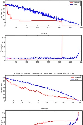
3.3.3 Diﬃcult examples increase model complexity

To demonstrate this point we again order the examples in terms of diﬃculty as in the

previous section. We measure the observed complexity of the model after training

on nested subsets of the training data by adding more and more diﬃcult examples.

As we noticed in the previous section we can observe better generalization error after

training without the most diﬃcult examples. In ﬁgure 3.4 we can see what the reason

might be. We plot the number of Support Vectors as a measure of complexity for each

nested subset of ordered training examples,as well as for random subsets of the same

size. We can notice that for some datasets we observe unduly increase in the measures

of complexity. For example,adding the last 15 most diﬃcult examples for Wisconsin

cancer data would signiﬁcantly increase the number of support vectors used as well

as the generalization error,ﬁgure 3.4. Again this results give intuition why some

examples might be troublesome and causing overﬁtting. Alternative measure of the

complexity actually used by SVM can be deﬁned by R_γ22 [4],whereγ is the margin and

R is the radius of the sphere which encompasses all the points. For Neural Networks

(35)

50 100 150 200 250 300 350 0 5 10 15 20 25 30 35

Complexity measure for random and ordered sets, Wisc. cancer data, 0% noise

Number SVs

ordered rand

50 100 150 200 250 300 350

0 0.1 0.2 0.3 0.4 0.5 Test error Test error

20 40 60 80 100 120 140 160 180

0 10 20 30 40 50 60 70

Complexity measure for random and ordered sets, Ionosphere data, 0% noise

Number SVs

ordered rand

20 40 60 80 100 120 140 160 180

[image:35.595.183.465.83.508.2]

0 0.1 0.2 0.3 0.4 0.5 Test error Test error

Figure 3.4: Inherent model complexity is increased by adding more diﬃcult examples. Top plot in each ﬁgure shows the number of Support Vectors for examples entering in increased complexity and for random set of the same size. Bottom plot shows correspondent test errors. Wisconsin cancer data (top) and Ionosphere data (bottom).

Many researchers working on generalization bounds [3],[26],[35],[38] have found

out that a better bound on the expected error might be estimated if some examples

(36)

the following theorem from [3] and [38] gives a trade-oﬀ between model complexity

and number of wrongly learned examples.

Theorem 3.3.1 Let F be a class of functions. With probability (w.p.) at least 1−δ

over m iid samples x from some fixed probability distribution P the following holds:

if f ∈ sgn(F) has margin at least γ on the examples x then the expected error of f

satisfies:

P(f(X)=Y)≤ _m2(dln34em

d log2(578m) +ln

4

δ)

For any other f ∈sgn(F) (which may have errors on x) w.p. at least 1-δ:

P(f(X)=Y)≤Pγ

m(f(X)=Y) +

2

m(dln

34em

d log2(578m) +ln

4

δ)

where d = f atF(γ/16) and Pmγ(f(X) = Y) is the portion of examples with margin

less than γ.

A similar bound for combination of classiﬁers,for example AdaBoost,was given

by Schapire et al. [35]: w.p. at least 1-δ.

P(f(X)=Y)≤Pγ

m(f(X)=Y) +

c m(

dln2(m/d)

γ2 +ln(1δ)),

where d is the VC dimension of the base classiﬁer.

The inﬂuence of diﬃcult or impossible to learn examples can be diminished by

imposing a simpler model or rather a trade-oﬀ of the model complexity and ﬁtting

the data well. This is again another form of regularization.

Unfortunately,for our example elimination tasks,those bounds are post factum,

meaning they estimate what the generalization error bound would be after the

algo-rithm has failed to learn some of the examples,or after certain margin is observed.

They are not constructive in the sense that they do not give ways to identify the

ex-amples which are troublesome so that the algorithm can beneﬁt from ignoring them

before starting to learn on them. The bounds are loose and can be used for

gen-eral penalty in model selection [3],[27],but are not precise enough to estimate best

(37)

Generally,those bounds are useful because they state that it might be reasonable

that some examples be removed if their presence in the training data increases unduly

the expended model complexity. What is needed is to have a constructive way to ﬁnd

out which are exactly the examples to be removed.

3.3.4 Regularization can beneﬁt from data pruning

Regularization methods are a very successful way to ignore or decrease the inﬂuence of

some noisy examples. By penalizing overly complex models a trade-oﬀ between model

complexity and number of examples not learned by the algorithm can be achieved.

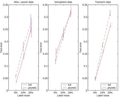
However,in the ﬁgures we have seen above,ﬁgure 3.2,we have a regularized

algorithm (SVM with slack variables,called SVC) which can still beneﬁt from pruning

of some noisy examples. We can observe that there are subsets of the data which would

improve generalization error. Thus,there might be examples which are so diﬃcult

that even though the algorithm has intrinsic mechanisms to cope with noise,they

might still inﬂuence it in an adversary way.

3.3.5 Challenges for data pruning

In this subsection we analyze important issues of what challenges and constraints we

have to face when dealing with noisy examples.

Model dependent or model independent deﬁnition of a diﬃcult example

In most of the cases in practice,algorithms,provided that they are of comparable

power,would share discriminatory boundaries on the same data,so the diﬃcult

ex-amples for one model would also be diﬃcult for the other,see ﬁgure 3.5. So,criterions

for pruning which depend on other models would also give satisfactory results. See,

for example,ﬁgure 3.3,where criterions for ordering in terms of diﬃculty based on

Neural Networks,SVM and AdaBoost can be used for decreasing the error with a

diﬀerent learning model,here SVM or AdaBoost. In general,however,the examples

(38)

to fit by another model. On figure 3.6 we show SVM model with different kernels on

the same dataset: SVM model with polynomial kernel would be inﬂuenced by some

examples and have larger test error if using the whole data while SVM with RBF

kernel can cope with those examples.

It seems a general criterion should depend on the learning model but if there are

particularly bad examples in the dataset they would be troublesome whatever model

is used,so,in practice a model diﬀerent from the target learning model can be used

to do the pruning.

−20 −15 −10 −5 0 5 10 15 20 −20 −15 −10 −5 0 5 10 15 20

SVM classification: Training points,SVs are marked with diamond

−20 −15 −10 −5 0 5 10 15 20 −20 −15 −10 −5 0 5 10 15 20

[image:38.595.183.464.251.368.2]

AdaBoost decision boundary, superimposed on the training set

Figure 3.5: Algorithms may share boundaries on the same datasets and therefore dif-ﬁcult examples. Decision boundaries for Support Vector Machine (left) and AdaBoost (right) on the same data.

Deﬁnition of diﬃcult examples depends on the whole data

As we discussed earlier,the deﬁnition of an outlier depends on the remaining

ex-amples and that a general penalty on the whole data may solve only partially the

problem. So,we believe we need to consider examples individually for elimination

but in the context of the rest of the data.

Training data is insuﬃcient

Learning from examples is an ill-posed problem in the ﬁrst place because of the

ﬁniteness of the training data and the fact that it is not known what class of functions

the target belongs to. If the data is noisy then the problem is even less well deﬁned.

With data pruning,we would like to investigate a more complicated problem,namely,

(39)

0 50 100 150 200 250 300 350 400 450 0 0.1 0.2 0.3 0.4 0.5 0.6 0.7 0.8

Learning with adding difficult examples, SVM−Poly, Wisconsin Cancer data

Test error

0 50 100 150 200 250 300 350 400 450 0 0.1 0.2 0.3 0.4 0.5 0.6 0.7 0.8

Learning with adding difficult examples, SVM−Rbf, Wisconsin Cancer data

Test error

[image:39.595.114.538.74.251.2]

Figure 3.6: Definition of difficult example depends on the model. Test error for ordered and random sets for SVM with Polynomial kernel (left) and with RBF kernel (right) on the same data. The left plot is taken from fig. 3.2. It is given here for the sake of comparison with another learning model.

where we do not know if and how much noise is present.

In many of the cases coping with noisy examples is done by relying on large amount

of data: RANSAC [16],query with noise [2],[23],etc. We are not entitled to using

more examples than the ones given.

Model and model complexity is unknown

Unlike probabilistic approaches here we cannot model the data. We take

discrimi-native approach in which the general model is ﬁxed but its complexity is unknown.

For example we may want to use Neural Networks but we have to select or learn

the topology of the network as well as some parameters on it. This gives additional

complications,because overly complex models would ﬁt the training data perfectly,

i.e.,would overﬁt with respect to the diﬃcult examples and would consequently have

poor generalization. Models which are too simple would not be learning the data well

(40)

3.4 Data pruning

3.4.1 Overview of the approach

Given the dataset and the learning model we want to ﬁnd out if there are examples

in the training data such that the learning algorithm would give possibly better

generalization error when training without them.

Our approach consists in randomizing the data so that to select multiple classiﬁers

which are of comparable power to the target learner and are diverse enough to have

semi-independent classification. These classifiers would be affected in different ways

by the troublesome examples. Probabilistic inference with naive Bayes classiﬁer is

done over the multiple classiﬁers’ opinions to decide which examples are troublesome.

3.4.2 Multiple models and data subsets are needed

Suppose the training data has troublesome examples and we knew the appropriate

model complexity. If the learning algorithm is applied to the whole data then it would

be inﬂuenced in an adversary way by these examples and would overﬁt or create a

poor discriminatory boundary. The trouble is that we do not know which examples

are actually causing the poor behavior. If we measure how well the examples do with

respect to the decision boundary it would not be correct because the algorithm may

have overﬁtted and learned those outlying examples very well. This problem is well

known in robust statistics [43].

One possible solution is to allow those troublesome examples to inﬂuence the

solutions in diﬀerent ways,i.e.,have both large and small inﬂuence. This can be

achieved by some sort of randomization of the training data. The correspondent

learners created from randomizing the data would be diverse and would be inﬂuenced

in diﬀerent ways by the troublesome examples. However,assuming that the outlying

examples are not the majority of the data,most of the learners would be consistent

with the target function. Thus the troublesome examples can be identiﬁed as the

(41)

3.4.3 Collecting multiple learners’ opinions

In the previous section we have argued that multiple diverse classiﬁers are needed to

be able to retrieve wrongly labeled or otherwise diﬃcult examples.

One way to create multiple semi-independent classiﬁers is through

bootstrap-ping [15]. It is appropriate for smaller size datasets and for small number of input

dimensions. Other ways of creating diversity of classiﬁers are through selecting

dif-ferent subsets of input features or selecting slightly overlapping subsets of the data

or even through injecting noise in the training data [10].

In this section we would stick to bootstrapping as one possible approach. Using

learners from bootstrapped data does not guarantee diversity but bootstrapping data

does encourage it [9].

Why bootstrapping? It is known that the existence of outliers in the data can

have detrimental effect on the final bootstrapped classifier because some resampled

subsets may have higher contamination levels even than the initial set [1]. This

might be a problem for creating a robust estimate by using bootstrapping,but would

be an important observation for our goals. Namely,if some diﬃcult examples would

inﬂuence some of the learners in an adversary way then using many other learners

which are not very badly inﬂuenced can identify this discrepancy.

Several explorations have shown that resampling with replicates gives an

imbal-ance in inﬂuence of certain random examples. The experiments of [12] show that

among multiple datasets created with bootstrapping there would be examples which

may not enter any resampled data as well as examples which would enter and inﬂuence

the committee multiple times. The important realization is that through

bootstrap-ping we can achieve an imbalance of inﬂuence of some random examples,but of course

we do not know which they would be. The authors of [12] as well as many others are

concerned with modiﬁying the bootstrapping sampling scheme so that to give equal

inﬂuence of each example. Conversely,we use bootstrapping to take advantage of the

imbalance of inﬂuence it gives. Our hope is that through multiple resamplings we

(42)

smaller extent the training set and therefore create classiﬁers which would be closer

or farther from the target.

Now,instead of aggregating the classiﬁers hoping to average out the poor eﬀect

of outliers on some classiﬁers,as often done in learning with ensembles [9],[18],we

would apply inference machine to ﬁnd out which examples have created discordant

classiﬁcations.

3.4.4 Pruning the data

So far we have retrieved multiple semi-independent learners which can classify the

data. The label and the conﬁdence of classiﬁcation of each learner,which we refer to

as a response of a classiﬁer,can be used as opinion of which example is diﬃcult and

its level of diﬃculty. The responses of the classiﬁers can be considered as projections

of the initial data.

Now we want to combine the classiﬁers responses or opinions of which example is

diﬃcult in an appropriate way.

3.4.4.1 Combining classiﬁers’ votes

Instead of simple voting we suggest to use inference with probabilistic models to

determine the true label of an example. We are interested in ﬁnding the probability

p(y|X) of the label of an example y,given the data X. In fact the label would be

determined by the ratio P_P(₍y_y=1₌₀|_|X_X)₎.

P(y=c|X)∝P(X|y=c)P(y=c) where c∈ {0,1}denotes a class label.

P(y=1|X) P(y=0|X) =

P(X|y=1)P(y=1) P(X|y=0)P(y=0)

The ratio is compared to 1 and if larger or equal then the estimated label of an

example is 1,otherwise 0.

The probabilities P(y = 1) and P(y = 0) are set to our prior belief of the data.

They can be set to 1₂ if the examples come in approximately equal proportions.

In both expressions P(X|y = 0) and P(X|y= 1) can be modeled and estimated

(43)

After estimating the new labels,the examples whose labels disagree with the

original ones are pruned.

3.4.4.2 Naive Bayes classiﬁcation

A simplest way to model the data is to use Naive Bayes classiﬁer and decompose the

data into several independent attributes. In our case the attributes are the projections

of the input data on several classiﬁers: P(X|y=c) =_jJ₌₁P(Aj|y=c)

In order to use Naive Bayes,an assumption of the attributes being independent

is crucial. Quite often,however,the rule can be successfully applied even if the

attributes are not independent.

Note that we might have started with a probabilistic model in the beginning

to reason about which example is wrong. But this would require us to assume a

particular probabilistic model of both the data and the diﬃcult examples which we

cannot do with enough generality.

3.4.5 Why pruning the data?

In the previous section we have estimated which examples create most disagreement

among classiﬁers and therefore are most diﬃcult to learn. Those examples might come

from various sources. The simplest assumption is that there is an oracle which ﬂips a

coin and with certain probability provides a wrong label. The examples are assumed

to come from the genuine distributions. This is the classiﬁcation noise scenario of

Angluin and Laird [2]. In this case,the best way to proceed is to ﬂip the labels of

the examples identiﬁed as noisy. However,in real-life dataset this is not a realistic

assumption: the examples may come from diﬀerent distributions,may be result of

measurement errors,may have errors introduced in the data component not only in

the label.

So,as we do not know the source of those troublesome examples,we suggest to

eliminate them from the data,i.e.,do data pruning. We consider it more dangerous

Data pruning

Anelia Angelova

Acknowledgements

Abstract

Contents

List of Figures

List of Tables

Chapter 1

Introduction

1.1

Learning and Generalization

1.2

Diﬃcult examples and outliers

1.3

Data pruning overview

1.3.1

What is data pruning?

1.3.2

Overview of data pruning method

Chapter 2

Identifying noisy examples

2.1

Introduction

2.1.1

What is a diﬃcult example?

2.1.2

How to deal with outliers?

2.1.3

Why deﬁning outliers is diﬃcult?

2.1.4

Motivation: Why study outliers?

2.2

Robust statistics

2.2.1

Accommodating outliers

2.2.2

Eliminating outliers

2.2.3

RANSAC

2.3

Regularization methods

2.3.1

Regularization with penalties

2.3.2

Introducing slack variables

2.3.3

Case study: Regularizing AdaBoost

2.4

Learning with queries

2.4.1

Learning in the presence of classiﬁcation noise

2.4.2

Learning in the presence of malicious noise

2.4.3

Active learning

2.5

Outliers in a probabilistic setting

2.6

Data valuation

2.6.1

Exhaustive learning

2.6.2

ρ

-criterion

Chapter 3

Data pruning

3.1

Introduction

3.2

Problem formulation

3.3

The essence of data pruning problem

3.3.1

When is data pruning necessary?

3.3.2

Beneﬁts of data pruning

3.3.3

Diﬃcult examples increase model complexity

3.3.4

Regularization can beneﬁt from data pruning