arXiv:1903.02075v3 [math.NA] 9 Mar 2019
Poisson data∗
Qingping Zhou†, Xiaoqun Zhang‡, and Jinglai Li§
Abstract. We provide a complete framework for performing infinite-dimensional Bayesian inference and uncer-tainty quantification for image reconstruction with Poisson data. In particular, we address the fol-lowing issues to make the Bayesian framework applicable in practice. We first introduce a positivity-preserving reparametrization, and we prove that under the reparametrization and a hybrid prior, the posterior distribution is well-posed in the infinite dimensional setting. Second we provide a dimension-independent MCMC algorithm, based on the preconditioned Crank-Nicolson Langevin method, in which we use a primal-dual scheme to compute the offset direction. Third we give a method based on the model discrepancy to determine the regularization parameter in the hybrid prior. Finally we propose to use the obtained posterior distribution to detect artifacts in a recovered image. We provide an application example to demonstrate the effectiveness of the proposed method.
Key words. Bayesian inference, image reconstruction, Markov chain Monte Carlo, Poisson distribution, total variation, uncertainty quantification.
AMS subject classifications. 45Q05, 62F15, 65C05, 68U10, 94A08
1. Introduction. Image reconstruction involves constructing interpretable images of ob-jects of interest from the data recorded by an imaging device [16]. Image reconstruction is usually cast as an inverse problem as one wants to determine the input to a system from the output of it. In most practical image reconstruction problems, the measurement and recording process is inevitably corrupted by noise, which renders the obtained data random. The statistical properties of the data have significant impact to the reconstruction results. In this work we shall focus on a special type of medical image reconstruction problems where the recorded data follows a Poisson distribution. The Poisson data usually arises in imaging prob-lems where the unknown quantity of interest is an object which interacts with some known incident beam of photons or electrons [21]. A very important example of such problems is the Positron emission tomography(PET) [27,3], a nuclear medicine imaging technique that is widely used in early detection and treatment follow up of many diseases, including cancer. In PET, the detection of signal is essential a photon counting process and as a result the data is well modeled by a Poisson distribution [3, 21]. The problem has attracted considerable research interests, and a number of methods have been developed to recover the image, e.g.,
∗Submitted to the editors DATE.
Funding: This work was funded by the National Natural Science Foundation of China, under grant numbers 11771288 and 11771289.
†School of Mathematical Sciences, Institute of Natural Sciences, Shanghai Jiao Tong University, 800 Dongchuan
Rd, Shanghai 200240, China, ([email protected]).
‡Institute of Natural Sciences, School of Mathematical Sciences, and the MOE Key Laboratory of
Scien-tific and Engineering Computing, Shanghai Jiao Tong University, 800 Dongchuan Rd, Shanghai 200240, China, ([email protected])..
§Corresponding Author, Department of Mathematical Sciences, University of Liverpool, Liverpool, L69 7ZL, UK
[32,35,15], just to name a few.
On the other hand, the stochastic nature of the data also introduces uncertainty into the image reconstruction process, and as a result the image obtained is unavoidably subject to uncertainty. In practice, many important decisions such as diagnostics have to be made based on the images obtained. It is thus highly desirable to have methods that can not only compute the image but also quantify the uncertainty in the image obtained. To this end, the Bayesian inference method has become a popular tool for image reconstruction [23], largely thanks to its ability to quantify uncertainty in the obtained image. The Bayesian formulation has long been used to solve image reconstruction problems with Poisson data, e.g., [20, 25, 19]. We note, however, that most of the works in the early years focus on computing a point estimate, which is usually the maximum a posteriori (MAP) estimate in the Bayesian setting, because of the limited computational power available then. More recently, mounting interest has been directed to the computation of the complete posterior distribution, rather than a point estimate, of the image, for that it can provide the important uncertainty information of the reconstruction results. For example, a Markov chain Monte Carlo (MCMC) algorithm is developed to sample the posterior distribution of the image in [5], and a variational Gaussian approximation of the posterior is proposed in [2].
used here has the total variation (TV) term which can be non-differentiable. To overcome this difficulty we modify the pCNL method by replacing the gradient direction with one com-puted by the primal-dual algorithm. We note that a similar problem is considered in [29,14] where a proximal method is used to approximate the gradient direction. Other than that the directions are computed with different approaches, another main difference between the aforementioned works and the present one is that we use the pCN framework here so the algorithm is dimension independent, while the works [29,14] concern finite dimensional prob-lems where discretization refinement is not an issue. Third, an important issue in the TG hybrid prior is to determine the value of the regularization parameter of the TV term. In the Bayesian framework, such parameters are often determined with the hierarchical Bayes or the empirical Bayes method [18]. As discussed in Section 4, these methods, however, are computationally intractable in our problem as we do not know the normalization constant of the TG prior. Thus, in this work we provide a method to determine the value of the TV regularization parameter based on the realized discrepancy model fit assessment approach developed in [17]. Finally, we provide an application of the uncertainty information obtained in the Bayesian framework, where we use the posterior distribution to detect possible artifacts in any reconstructed image.
The rest of the paper is organized as the following. In Section 2, we present the infinite dimensional Bayesian formulation of the image reconstruction problem with Poisson data, and we prove that under the reparametrization the resulting posterior is well-posed in the function space. In Section 3, we describe the primal-dual pCN algorithm to sample the posterior distribution of the present problem. Section 4 provides a method to determine the value of the regularization parameter in the TG prior. Section 5 discusses how to use the posterior distribution to detect artifacts in a reconstructed image. Finally numerical experiments of the proposed Bayesian framework are performed in Section 6.
2. Infinite dimensional Bayesian image reconstruction with Poisson data. In this sec-tion, we formulate the image reconstruction with Poisson data in an infinite dimensional Bayesian framework.
2.1. The Bayesian inference formulation for functions. We start by presenting a generic Bayesian inference problem for functions. Let X be a separable Hilbert space of functions with inner product h·,·iX. Our goal is to inferu∈X from data y∈Y ⊆Rd and y is related to u via the likelihood function π(y|u), i.e., the distribution of y conditional on the value of
u. In the Bayesian setting, we first assume a prior distribution µpr of the unknownu, which represents one’s prior knowledge on the unknown. In principle µ0 can be any probabilistic measure defined on the space X. The posterior measure µy of u conditional on data y is provided by the Radon-Nikodym(R-N) derivative:
(2.1) dµ
y
dµpr
(u) =π(y|u),
which can be interpreted as the Bayes’ rule in the infinite dimensional setting. The posterior distributionµy thus can be computed from Eq. (2.1) with, for example, a MCMC simulation.
from the underlying mathematical model relating the data and to the unknown image. We assume that the image is first projected to the noise-free observable via a mappingA:X →Y,
(2.2) θ = Au.
While noting that the proposed framework is rather general, here for simplicity we restrict ourselves in the case whereAis a bounded linear transform. For example in the PET imaging problems, the mappingA is the Radon transform, where each θi is computed by integrating
u(x) alone a lineLi:
(2.3) θi = (Au)i =K
Z
Li
u(x)|dx|,
fori= 1, ..., d, whereKis a positive constant describing the noise level. The Radon transform is a bounded linear transform [26]. Poisson noise is then applied to theprojected observable θ, yielding the likelihood function π(y|u) =πP(y|θ = Au), whereπP(y|θ) is the d-dimensional Poisson distribution:
(2.4) πP(y|θ) =
d
Y
i=1
(θi)yiexp(−θi)
yi!
.
In the PET problem, there is an additional restriction: the unknown function u must be positive. The reason is two-fold: first from the physical point of view, the unknownu repre-sents the density of the medium, which is positive; from a technical point of view, if u is not constrained to be positive, it may yield some negative components of the predicted data θ, which renders the Poisson likelihood un-defined. To this end, we need to introduce a trans-formation to preserve positivity of the unknown u. To impose the positivity constraint, we reparameterize the unknownu as:
u(x) =f(z(x)) = a
2(erf(z(x)) +b),
where a and b are two constants satisfying a > 0 andb > 1, and erf(·) is the error function defined as:
erf(z) = √2
π Z z
0
e−t2dt.
With the new parametrization, it is easy to see that for any x∈Ω, we have
(2.5) 1
2a(b−1)≤u(x)≤ 1
2a(b+ 1).
Now we can infer the new unknown z and once z is known u can be computed accordingly. In this setup, the likelihood function forz becomes
π(y|z) =πP(y|θ= Af(z))
where πP(y|θ) is the d-dimensional Poisson distribution given by Eq. (2.4). Following [33], we can write the likelihood function π(y|z) in the form of
where
(2.6b) Φ(z;y) =
d
X
i=1
(Af(z))i−yiln(Af(z))i.
For simplicity we can rewrite Eq. (2.6b) as,
(2.7) Φ(z;y) =hAf(z),1i − hy,ln(Af(z))i=hθ,1i − hy,lnθi,
where 1 is ad-dimensional vector whose components are all one,θ = Af(z) is the predicted observable, andh·,·idenotes the Euclidean inner product. In what follows we often omit the argument y and simply use Φ(z), when not causing ambiguity. This notation will be used often later.
2.3. Bayesian framework with the hybrid prior for PET imaging. We now describe how the infinite dimensional Bayesian inference framework is applied to the PET problem. First we assume that the unknown functionzis a function defined on Ω, a bounded open subset of
R2. In particular, we set the state space X to be the Sobolev spaceH1(Ω):
X =H1(Ω) ={z(x)∈L2(Ω)|∂x1z, ∂x2z∈L2(Ω) for allx= (x1, x2)∈Ω}.
The associated normk · kX =k · kH1 is
kzk2H1 =kzk2L
2(Ω)+k∂x1zk
2
L2(Ω)+k∂x2zk
2
L2(Ω).
Choosing a good prior distribution is one of the most important issues in Bayesian inference. Conventionally one often assumes that the prior on z, is a Gaussian measure defined on X
with mean ξ covariance operator C0, i.e. µpr =µ0 =N(ξ, C0). Note that C0 is symmetric positive and of trace class. The Gaussian prior has many theoretical and practical advantages, but a major limitation of the Gaussian prior is that it can not model functions with sharp jumps well.
To address the issue, here we use the TV-Gaussian prior proposed in [36]:
(2.8) dµpr
dµ0
(z)∝exp(−R(z)), R(z) =λkzktv.
wherek · kTV is the TV seminorm,
(2.9) kzkTV=λ
Z
Ωk∇
uk2dx,
andλis a positive constant. It follows immediately that the R-N derivative ofµy with respect to µ0 is
(2.10) dµ
y
dµ0
(z)∝exp(−Φ(z)−R(z)),
Next we shall show that the formulated Bayesian inference problem is well defined in the infinite dimensional setting. We first show that Φ(z) given by Eq. (2.7) satisfies certain important conditions, as is stated by Proposition 2.1.
Proposition 2.1. The functional Φgiven in Eq. (2.7) has the following properties:
1. For every r >0, there are constants M(r)∈R and N(r)>0 such that, for all z∈X , and y∈Y with kyk2< r,
M ≤Φ(z)≤N;
2. For every r >0 there is a constantM(r)>0 such that, for all z, v∈X with
max{kzkX,kvkX}< r,
|Φ(z)−Φ(v)| ≤Mkz−vkX;
3. There exists a constant M >0 such that for any y, y′ ∈Y, we have
|Φ(z;y)−Φ(z;y′)| ≤Mky−y′k2.
A detailed proof of the proposition is provided in AppendixA. Following Proposition2.1, we can conclude that the hybrid prior (2.8), and the log-likelihood function Eq. (2.7) yield a well-behaved posterior measure given by Eq. (2.10) in the infinite-dimensional setting, as is summarized in the following theorem:
Theorem 2.2. For Φ(z) given by Eq. (2.7) and prior measure µpr given by Eq. (2.8), we
have the following results:
1. µy given by Eq. (2.10) is a well-defined probability measure on X.
2. µy given by Eq.(2.10)is Lipschitz in the data y, with respect to the Hellinger distance: ifµy andµy′
are two measures corresponding to datay andy′the there existsC =C(r)
such that, for all y, y′ withmax{kyk2,ky′k2}< r,
dHell(µy, µy ′
)≤Cky−y′k2.
3. Let
(2.11) dµ
y N1,N2
dµ0
= exp(−ΦN1(z)−RN2(z)),
whereΦN1(z)is a N1∈Ndimensional approximation ofΦ(z) andRN2(z) is aN2 ∈N
dimensional approximation of R(z). Assume that ΦN1 satisfies the three properties
of Proposition 2.1 with constants uniform in N1, and RN2 satisfy Assumptions A.2
(i) and (ii) in [36] with constants uniform in N2. Assume also that for ∀ǫ > 0,
there exist two positive sequences{aN1(ǫ)} and{bN2(ǫ)} converging to zero, such that
µ0(Xǫ)≥1−ǫ for ∀N1, N2 ∈N, where
Xǫ ={z∈X| |Φ(z)−ΦN1(z)| ≤aN1(ǫ),|R(z)−RN2(z)| ≤bN2(ǫ)}.
Then we have
Theorem2.2 is a direct consequence of Proposition2.1, and the proof of the theorem can be found in [36] and is omitted here.
Finally, we note that, in the numerical implementations, we use the truncated Karhunen-Lo`eve (KL) expansion [24] to represent the unknownz. Namely, we writezas
(2.12) z(x) =
N
X
i=1
zi√ηiei(x),
where {ηi, ei(x)} are the eigenvalue-eigenfunction pair of the covariance operator C0, and (z1, ..., zN) are independent with each following a standard normal distribution. In the KL representation, the number of KL modes (eigenfunctions)N corresponds to the discretization dimensionality.
3. The primal-dual preconditioned Crank-Nicolson MCMC algorithm. In most practical image reconstruction problems, the posterior distribution can not be analytically calculated. Instead, one usually represent the posterior by samples drawn from it using MCMC algo-rithms. It is demonstrated in [13] that standard MCMC algorithms may become problematic in the infinite dimensional setting: its acceptance probability will generate to zero as the discretization dimensionality increases. Here we adopt the pCN MCMC algorithm particu-larly developed for the infinite dimensional problems [13]. An important feature of the pCN MCMC algorithm is that its sampling efficiency is independent of discretization dimensional-ity up to the numerical errors in the evaluation of the functionalsR(·) and Φ(·), which makes it particular useful for sampling the posterior distribution defined in function spaces. We start with a brief introduction of the pCN algorithm following the presentation of [13]. We denote Φ(z)+R(z) of Eq. (2.10) as Ψ(z). Simply speaking the algorithms are derived by applying the Crank-Nicolson (CN) discretization to a stochastic partial differential equation whose invari-ant distribution is the posterior. We here omit the derivation details while referring interested readers to [13], and jump directly to the pCN proposal:
(3.1) v = (1−β2)12z+βw,
where z and v are the present and the proposed positions respectively, w ∼ N(ξ, C0) and
β ∈ [0,1] is the parameter controlling the stepsize of the algorithm. The proposed sample v
is then accepted or rejected according to the acceptance probability:
(3.2) a(v, z) = min{1,exp [Ψ(z)−Ψ(v)]},
which is independent of discretization dimensionality up to numerical errors.
The pCN proposal in Eq. (3.1) can be improved by incorporating the data information in the proposal, and following the idea of Langevin MCMC for the finite dimensional problems, one can derive the preconditioned Crank-Nicolson Langevin (pCNL) proposal:
(3.3) (2 +δ)v= (2−δ)z−2δC0DΨ(z) + √
8δw,
whereδ ∈[0,2],w∼N(ξ,C0) andDis the gradient operator. If we defineρ(z, v) as following:
(3.4) ρ(z, v) = Ψ(z) +1
2hv−z,DΨ(z)i+
δ
4hz+v,DΨ(z)i+
δ
4kC 1/2
then the acceptance probability is given by:
(3.5) a(z, v) = min{1,exp (ρ(z, v)−ρ(v, z))}.
The pCNL algorithm is usually more efficient than the standard pCN algorithm as it takes advantage of the gradient information of the Ψ(z). However, the pCNL algorithm can not be used directly in our problem as Ψ(z) includes the TV term which is not differentiable. It is important to note that −2δC0DΨ(z) is the offset term only affecting the mean of the proposal, and we can replace DΨ(z) with another directiong(z), yielding proposal:
(3.6) (2 +δ)v= (2−δ)z−2δC0g+ √
8δw,
where δ ∈ [0,2] and w ∼ N(ξ,C0). And it can be verified that the detailed balance is maintained if we change Eq. (3.4) to
(3.7) ρ(z, v) = Ψ(z) + 1
2hv−z, gi+
δ
4hz+v, gi+
δ
4kC 1/2 0 gk2,
while the acceptance probability is given by Eq. (3.5). Now we need to find a good direction
g(z). In [29] the authors use Moreau approximation to approximate the TV term in the Langevin MCMC algorithm. Here we shall provide an alternative approach, determining the offset direction in the MCMC iteration using the primal dual algorithm. The primal-dual algorithms are known to be very effective in solving optimization problems involving TV regularization [11,12,10], and we hereby give a brief description of the primal dual method applied to our problem. Suppose that we want to solve
(3.8) min
z∈XΨ(z) = Φ(z) +λkzkTV.
Introducing a new variable φ(x) = [φ1(x), φ2(x)] with φ1(x), φ2(x) ∈L2(Ω) (we denote this asφ∈L2
2(Ω)), and we then rewrite the optimization problem (3.8) as min
z∈X,φ∈L2
2(Ω)
Ψ(z, φ) = Φ(z) +λkφk2,1 (3.9)
s.t. Dz=φ,
wherekφk2,1 =
kφ1(x)k2L2(Ω)+kφ2(x)k2L2(Ω)
1/2
. The augmented Lagrangian for Eq.(3.9) is
(3.10) max
η∈L2
2(Ω)
min z∈X,φ∈L2
2(Ω)
Lρ(z, φ, η) = Φ(z) +λkφk2,1+hη,Dz−φi+ρ
2kDz−φk 2 2,
where η ∈ L22(Ω) is the dual variable or Lagrange multiplier, and ρ > 0 is a constant called the penalty parameter. The resulting problem is then solved with the Alternating Direction Method of Multipliers (ADMM) [7]:
zk+1 = arg min
z∈X Lρ(z, φ k, ηk), (3.11a)
φk+1 = arg min φ∈Lq2(Ω)
Lρ(zk+1, φ, ηk), (3.11b)
ηk+1 =ηk+ρ(φk+1−Dzk+1).
The algorithm consists of a z-minimization step (3.11a), a φ–minimization step (3.11b), and a dual ascent step (3.11c). When applied to the MCMC algorithm, the iterations proceed as described in in Algorithm 3.1. It should be noted here that, in Step 3 of the algorithm, it is required to solve a minimization problem. However, for efficiency’s sake, we choose not to solve this optimization accurately. In the numerical implementations in this work, we only perform one gradient descent iteration, and so the computational cost for each MCMC iteration does not increase much compared to standard pCN.
Algorithm 3.1 The Primal-dual pCN(PD-pCN) algorithm
1: Initialize z0, φ0, η0
2: fork= 0,1,2,· · · do
3: z∗= arg min
z∈X Lρ(z, φk, ηk);
4: g=z∗−zk;
5: Propose v using Eq. (3.6) 6: Draw θ∼U[0,1];
7: Computea(z, v) with Eq. (3.5) and Eq. (3.7); 8: if θ≤a then
9: zk+1 =v;
10: φk+1= arg minφ∈Lq
2(Ω) Lρ(z
k+1, φ, ηk);
11: ηk+1=ηk+ρ(φk+1−Dzk); 12: else
13: zk+1 =zk;
14: φk+1=φk; 15: ηk+1=ηk; 16: end if
17: end for
4. Determining the TV regularization parameter. Just like the deterministic inverse problems, it is an important issue to determine the TV regularization parameter λ in the hybrid prior. In the Bayesian setting, standard methods such as the empirical Bayes (EB) approach [18] can be too computationally intensive in the present problem, especially as we have no knowledge of the normalization constant of the hybrid prior. Namely, recall that the EB method seeks to maximize
π(y|λ) =
Z
π(y|u)µpr(du) =
Z
π(y|u) 1
Z(λ)exp(−λkukTV)µ0(du)
where Z(λ) is not known in advance and needs to be evaluated with another Monte Carlo integration. Here we provide a statistical approach to determine the value of λ, which is derived from the realized discrepancy method for model assessment proposed in [17].
use the χ2 discrepancy,
(4.1) D(y,θ) =
d
X
i=1
(yi−θi)2
θ2
i
.
Now knowing thatθ= Au, we can use this discrepancy to assess how well a specific choice of
u fits the data. The classical p-value based on the discrepancy D(y,θ) is
(4.2) pc(y,θ) =P[D(y,θ)> D(˜y,θ)]
where ˜y is the simulated data from model (2.4). In particular, for the discrepancy function given in Eq. (4.1), thep-value is simply,
(4.3) pc(y,θ) = 1−Fχ2
d(D(y,θ)), whereFχ2
d(·) is the cumulative distribution function of theχ
2 distribution with the degree of
freedomd. The classic p-value computed this way provides an assessment of how well a single estimate of u fits the datay. The method can be extended to the Bayesian setting to assess the fitness of the posterior distribution to data. First recall that our prior distribution given by Eq. (2.8) is specified by the parameter λ, and as a result the posterior also depends on λ
and here we write the posterior asµyλ(du) to emphasize its dependence on λ. In the Bayesian setting, one can compute the posterior predictivep-value:
(4.4) pb(y, λ) =
Z
pc(y,θ)p(θ|y, λ)dθ =
Z
pc(y,Au)µyλ(du),
5. Artifact detection using the posterior distribution. In practical image reconstruction problems, due to the imperfection of methods or devices, a reconstructed image may contain artifacts what are not present in the original imaged object. In this section we describe an application of the posterior distribution to detect artifacts in a reconstructed image.
Specifically, we consider the posterior distribution of the image at any given pointx, which is denoted asux. Consequently we can write the posterior distribution ofuxasπx(ux|y). Next
we consider the highest posterior density interval (HPDI) which is essentially the narrowest interval corresponding to a given confidence level. More precisely, for an α ∈ [0,1], the 100(1−α)% HPDI is defined as (cite)
Cα ={u(x)|πx(u(x)|y)> πα}
where πα is the largest constant satisfying P[ux|πx(ux|y) > πα] = 1−α. Now suppose that
we have a reconstruct image ˆuand we also write its value at x as ˆux. Next we shall estimate
how large the credible level (1−α) must be so that the associated HDPI may contain ˆux.
That is, we compute the smallest value of (1−α) such that,
ˆ
ux∈Cα.
Intuitively speaking, the larger the computed credible level (1−α) is, the more likely the considered ˆux is an artifact. And we thus use the credible level (1−α) to measure how likely
a point is an artifact, and we can do this test for any pointx∈Ω. Alternatively, the problem can also be formulated as a Bayesian hypothesis test with a fixedα(e.g. α= 5%) [28]: that is, ˆ
u(x) is regarded to be an artifact if it is not contained in the (1−α) HPDI for the prescribed value of α. However, it has been pointed out in [34] that performing hypothesis test with HPDI may cause certain theoretical issue and so here we choose not to use the hypothesis test formulation.
It should be noted here that, in [30,14], the authors utilize the highest posterior density (HDP) region to test if a candidate image is likely to be a solution to the reconstruction problem. The purpose of the present work differs from the aforementioned ones in that we want to identify regions or pixels which are unlikely to be present in the original image, rather than to assess the entire image.
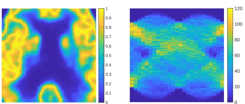
6. Numerical results. In this section we demonstrate the performance of the proposed Bayesian framework, by applying it to a PET image reconstruction problem with synthetic data. In particular the ground truth image (Fig. 1, left) is chosen from the Harvard whole brain atlas [1]. We let Ω = (0,1)2 and set the image size to be 128×128. In the Radon transform we use 60 projections equilaterally sampled from 0 to π. The test data, shown in the right figure of Fig. 1, is randomly simulated by plugging the true image into the Radon transform and the Poisson distribution (2.4) where the noise level K is taken to be 1. In the Bayesian inference, we use the hybrid prior distribution where the Gaussian part is taken to be zero mean and covariance:
(6.1) K(x,x′) =γexp
−kx−x ′
k1
d ,
0 0.1 0.2 0.3 0.4 0.5 0.6 0.7 0.8 0.9 1
[image:12.612.86.505.85.264.2]0 20 40 60 80 100 120
Figure 1: Left: the true image. Right: the noisy data.
6.1. Convergence with respect to discretization dimensionality. In the numerical imple-mentation we represent the unknownz using the truncated KL expansion withN KL-modes. First we shall demonstrate that the posterior distributions converges with respect to the dis-cretization dimensionalityN. To do so, we perform the proposed PD-pCN MCMC simulation and compute the posterior means with six different values ofN: Ni =i×103 fori= 1...6. We note here that, in all the MCMC simulations performed in this section, we fix the number of samples to be 5×10⁵ with additional 0.5×10⁵ samples used in the burn-in step, and also, in all the simulations the stepsizeβhas been chosen in a way that the resulting acceptance prob-ability is around 25%. We then compute the L2 norm of the difference between the posterior mean with N =Ni and that with N =Ni+1 for eachi= 1...6:
(6.2) Diff =
Z
Ω
(ˆuNi(x)−uˆNi+1(x))
2dx
where ˆuNi is the posterior mean ofu computed withNi KL modes. We plot theL2 difference against the discretization dimensionality N in Fig. 2 (left). One can see from the figure that the difference decrease as N increase and the difference becomes approximately zero for
N = 5000 and N = 6000, indicating the convergence of the posterior mean with respect to
N. For each posterior mean ˆuNi, we also compute its peak signal-to-noise ratio (PSNR) [22], a commonly used metric of the quality of a reconstructed image. We show the PSNR results in Fig. 2 (right), and the figure shows that the PSNR increases as N increases from 1000 to 4000, and remains approximately constant from 4000 to 6000, suggesting that increasing the discretization dimensionality can improve the inference accuracy until the posterior converges, and so it is important to use sufficiently large discretization dimensionality in such problems. In the rest of the work, we fixN = 6000.
al-1000 2000 3000 4000 5000 6000
N
0 0.02 0.04 0.06 0.08 0.1 0.12
Diff
1000 2000 3000 4000 5000 6000
N
14 15 16 17 18 19 20 21 22
[image:13.612.76.507.99.264.2]PSNR
Figure 2: Left: the convergence of the posterior mean. Right: the PSNR of the posterior mean as a function ofN.
0 50 100 150 200
lag
0.1 0.2 0.3 0.4 0.5 0.6 0.7 0.8 0.9
ACF
pCN PD-pCN
0 50 100 150 200
lag
0 0.2 0.4 0.6 0.8 1
ACF
pCN PD-pCN
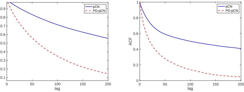
Figure 3: The ACF of the samples drawn by the pCN and the PD-pCN methods.
gorithms. We reinstate that in both algorithms we have chosen the step size so that the resulting acceptance probability is around 25%. We compute the auto-correlation function (ACF) of the samples generated by the two methods at two points: one in the center of the image, x= [0.5,0.5] and the other near the boundary of itx= [0.05,0.05]. We plot the ACF at the two points in Fig. 3, and one can see from the figure that at both points the ACF of the propose PD-pCN method decays much faster than that of the standard pCN. To further compare the performance, we compute the effective sample size(ESS):
ESS = N
1 + 2τ,
[image:13.612.89.494.330.483.2]0 1 1.1 1.2 1.3 1.4 1.5 1.6 1.7
ESS
104
row 64
[image:14.612.95.481.95.230.2]row 1 row 128
Figure 4: ESS of pCN and pCNL algorithms
λ 0 0.5 1 2 3 4
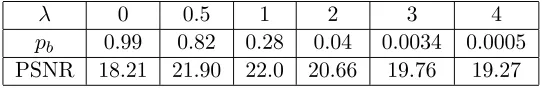
pb 0.99 0.82 0.28 0.04 0.0034 0.0005 PSNR 18.21 21.90 22.0 20.66 19.76 19.27
Table 1: The posterior predictive p-value (pb) and the PSNR of the resulting posterior mean for different values ofλ.
128. Just as the ACF, the results show that the PD-pCN algorithm achieves much higher ESS than the standard pCN. We have also examined the ESS of other rows where the results are qualitatively similar to those three shown in Fig. 4, and so we omit those results.
6.3. Determining parameter λ. As is discussed at the beginning of the section, the prior parameter λis determined with the realized discrepancy method discussed in Section 4. We here provide some details on the issue. Specifically we test five different values of λ: λ = 0,0.5,1,2,3, and using the method discussed in Section 4 we compute the corresponding posterior predictivep-value for each value ofλ, shown in Table 1. We can see from the table that, asλincreases, the resultingp-value decays. These results agree well with our expectation that asλbecomes larger, the prior distribution becomes stronger, and as a result thep-value which assesses the fitness of the posterior to the data becomes smaller. We also compute the PSNR of the posterior distribution computed with all theseλvalues, and the results are also given in the table. We can see here that, for both very large and very small p-values, the associated posterior means are of rather poor quality in terms of PSNR. That is, when the
p-value is too large, the posterior distribution overfits the data, and when it is too small, the posterior underfits the data; both cases lead to a poor performance of the inference, and so we must choose a proper p-value that represents a good balance of the prior and the data. Based on our numerical tests, we suggest that for the present problem it is suitable to use λ
where the associated p-value is in [0.1,0.5], and so here we chooseλ= 1 where the resulting
p-value is 0.28.
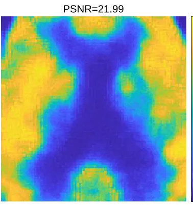
[image:14.612.158.429.272.316.2]PSNR=21.99
0 0.1 0.2 0.3 0.4 0.5 0.6 0.7 0.8 0.9 1
(a) The posterior mean of the TG prior.
0 0.1 0.2 0.3 0.4 0.5 0.6 0.7 0.8
(b) The interval width of 95% HPDI of the TG prior.
PSNR=18.21
0 0.2 0.4 0.6 0.8 1
(c) The posterior mean of the Gaussian prior.
0 0.1 0.2 0.3 0.4 0.5 0.6 0.7 0.8
[image:15.612.77.266.92.293.2](d) The interval width of 95% HPDI of the Gaussian prior.
Figure 5: A comparison of the posterior statistics of the TG and the Gaussian priors.
Gaussian prior corresponding to settingλ= 0 in the TG prior, and the results are also shown in Figs. 5 (Fig. 5c and Fig.5d). The figures show that the posterior mean obtained with the TG prior is clearly of better quality than that of the Gaussian prior, suggesting that including the edge-preserving TV term significantly improves the performance of the prior. It is worth noting here that, the Gaussian prior used here is not optimized for the best performance, and the performance can be potentially improved by using some carefully designed Gaussian priors, for example, [9].
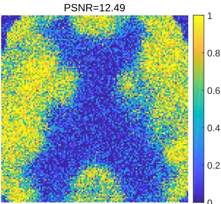
6.5. The impact of Poisson likelihood function. In practice, the observation noise is often assumed to be Gaussian, for that it usually leads to great convenience for computation. In what follows we shall demonstrate that, if the data is generated truly from a Poisson distribution, and if the noise is strong, the use of a Gaussian noise model may yield very poor reconstruction results. Recall that the datayused in this example is drawn from the Poisson model, and here we perform the Bayesian inference using a Gaussian likelihood:
(6.3) π(y|θ) =N(θ,Θ),
where Θ is a d×d diagonal matrix with each diagonal component to be θi for i = 1...d. By design the Gaussian likelihood (6.3) has the same mean and covariance as the original Poisson likelihood. We compute the posterior distribution using the Gaussian likelihood and the same prior as before, and we plot the posterior mean in Fig. 6. It can be seen clearly from the figure that the posterior mean computed with the Gaussian likelihood is of much poor quality than that of the Poisson likelihood (shown in Fig. 5a). The results can be also compared quantitatively: the PSNR of the posterior mean of Gaussian likelihood is calculated to be 12.49, while that of the Poisson likelihood is 21.99. The significant difference between the results of the Gaussian likelihood and the Poisson likelihood suggests that the use of the Gaussian likelihood function may result in poor reconstruction performance in problems with Poisson data.
PSNR=12.49
[image:17.612.182.405.93.299.2]0 0.2 0.4 0.6 0.8 1
Figure 6: The posterior mean of the Gaussian likelihood.
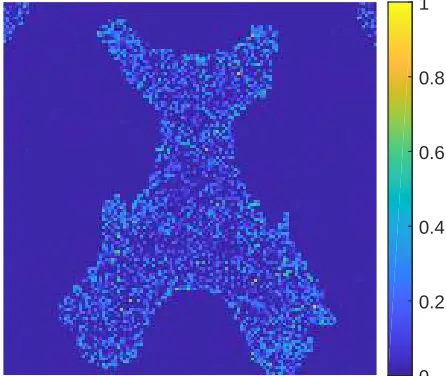
contain artifacts. The results demonstrate that the proposed method can rather effectively detect the artifacts in a test image.
7. Conclusions. In this work, we have presented a complete treatment for performing Bayesian inference and uncertainty quantification for image reconstruction problems with Poisson data. In particular, we formulate the problem in an infinite dimensional setting and we prove that the resulting posterior distribution is well-posed in this setting. Second, to sample the unknown function/image, we provide a modified pCNL MCMC algorithm, the efficiency of which is independent of discretization dimensionality. Specifically the modified algorithm calculates the offset direction in the original pCNL algorithm by using a primal-dual method, to avoid computing the gradient of the TV term in our formulation. Third, we also give a method to determine the TV regularization parameter λ which is critical for the prior distribution. The method is based on the realized discrepancy method for assessing model fitness. Finally we provide an application of the uncertainty information obtained by the Bayesian framework, using the posterior distribution to identify possible artifacts in an image reconstructed. We believe the proposed Bayesian framework can be used to recon-struct images and evaluate the uncertainty or credibility of the images reconrecon-structed in many practical imaging problems with Poisson data. In the future, we plan to further investigate the possibility of applying the methods developed in this work to those real-world problems, especially the PET image reconstruction.
Appendix A. Proof of Proposition. We provide a proof of Proposition 2.1 in the Appendix.
Proof. (1) SinceA is bounded, from Eq. (2.5), we obtain directly that
0 0.2 0.4 0.6 0.8 1
(a) Surrogate test image one.
0 0.2 0.4 0.6 0.8 1
(b) The credible level (1−α) computed for test image one.
0 0.2 0.4 0.6 0.8 1
(c) Surrogate test image two.
0 0.2 0.4 0.6 0.8 1
(d) The credible level (1−α) computed for test image two.
0 0.2 0.4 0.6 0.8 1
(e) Surrogate test image three.
0 0.2 0.4 0.6 0.8 1
[image:18.612.292.515.99.287.2](f) The credible level (1−α) computed for test im-age three.
for two constant vectorsθandθ. It follows directly thatklnθk2≤lmaxfor a positive constant
lmax.
For every r > 0, we have kyk2 < r. By the Cauchy-Schwarz inequality, we obtain the lower bound,
Φ(z) =hθ,1i − hy,lnθi
≥ hθ,1i − klnθk2kyk2
≥ hθ,1i −lmaxkyk2
≥ hθ,1i −lmaxr.
For upper bound, once again we apply the Cauchy-Schwarz inequality to the functional Φ, obtaining
Φ(z) =hθ,1i − hy,lnθi
≤ hθ,1i+klnθk2kyk2
≤ hθ,1i+lmaxkyk2
≤ hθ,1i+lmaxr.
(2) In this proof, we useM for positive constants. Letz andv be any two elements inX, and we have,
|Φ(z)−Φ(v)|=|hAf(z)−Af(v),1i − hy,ln(Af(z))−ln(Af(v))i| ≤ |hAf(z)−Af(v),1i|+|hy,ln(Af(z))−ln(Af(v))i| ≤ k1k2kAf(z)−Af(v)k2+kyk2kln(Af(z))−ln(Af(v))k2 ≤ k√dkAf(z)−Af(v)k2+kyk2MkAf(z)−Af(v)k2 = (√d+kyk2M)kAf(z)−Af(v)k2.
(A.1)
Since the mappingA is a bounded linear transform from theX to Y, we have,
(A.2) kAf(z)−Af(v)k2 ≤ kAkkf(z)−f(v)kL2
=kAkk Z z
v
e−t2dtkL2 ≤ kAkk
Z z
v
dtkL2 =kAkkz−vkL2,
which completes the proof.
(3) For any y, y′ ∈Y, it is easy to show,
|Φ(z, y)−Φ(z, y′)|=|hy−y′,lnθi| ≤ ky−y′k2klnθk2 ≤lmaxky−y′k2.
REFERENCES
[1] Johnson K A and Becker J. www.med.harvard.edu/aanlib/. Accessed April 4, 2010.
[3] Dale L Bailey, Michael N Maisey, David W Townsend, and Peter E Valk.Positron emission tomography. Springer, 2005.
[4] Johnathan M Bardsley and John Goldes. Regularization parameter selection methods for ill-posed poisson maximum likelihood estimation. Inverse Problems, 25(9):095005, 2009.
[5] Johnathan M Bardsley and Aaron Luttman. A metropolis-hastings method for linear inverse problems with poisson likelihood and gaussian prior. International Journal for Uncertainty Quantification, 6(1), 2016.
[6] Mario Bertero, Patrizia Boccacci, Giorgio Talenti, Riccardo Zanella, and Luca Zanni. A discrepancy principle for poisson data.Inverse problems, 26(10):105004, 2010.
[7] Stephen Boyd, Neal Parikh, Eric Chu, Borja Peleato, Jonathan Eckstein, et al. Distributed optimization and statistical learning via the alternating direction method of multipliers.Foundations and TrendsR
in Machine learning, 3(1):1–122, 2011.
[8] Steve Brooks, Andrew Gelman, Galin Jones, and Xiao-Li Meng. Handbook of markov chain monte carlo. CRC press, 2011.
[9] Daniela Calvetti and Erkki Somersalo. A gaussian hypermodel to recover blocky objects.Inverse problems, 23(2):733, 2007.
[10] Antonin Chambolle. An algorithm for total variation minimization and applications. Journal of Mathe-matical imaging and vision, 20(1-2):89–97, 2004.
[11] Antonin Chambolle and Thomas Pock. A first-order primal-dual algorithm for convex problems with applications to imaging. Journal of mathematical imaging and vision, 40(1):120–145, 2011.
[12] Tony F Chan, Gene H Golub, and Pep Mulet. A nonlinear primal-dual method for total variation-based image restoration. SIAM journal on scientific computing, 20(6):1964–1977, 1999.
[13] Simon L Cotter, Gareth O Roberts, AM Stuart, David White, et al. MCMC methods for functions: modifying old algorithms to make them faster. Statistical Science, 28(3):424–446, 2013.
[14] Alain Durmus, Eric Moulines, and Marcelo Pereyra. Efficient bayesian computation by proximal markov chain monte carlo: when langevin meets moreau.SIAM Journal on Imaging Sciences, 11(1):473–506, 2018.
[15] Jeffrey A Fessler. Penalized weighted least-squares image reconstruction for positron emission tomography.
IEEE transactions on medical imaging, 13(2):290–300, 1994.
[16] Jeffrey A Fessler. Medical image reconstruction: a brief overview of past milestones and future directions.
arXiv preprint arXiv:1707.05927, 2017.
[17] A Gelman. Posterior predictive assessment of model fitness via realized discrepancies (with discussion).
Statistica Sinica, 6(4):733–760, 1996.
[18] Andrew Gelman, Hal S Stern, John B Carlin, David B Dunson, Aki Vehtari, and Donald B Rubin.
Bayesian data analysis. Chapman and Hall/CRC, 2013.
[19] Peter J Green. Bayesian reconstructions from emission tomography data using a modified em algorithm.
IEEE transactions on medical imaging, 9(1):84–93, 1990.
[20] Tom Hebert and Richard Leahy. A generalized em algorithm for 3-d bayesian reconstruction from poisson data using gibbs priors. IEEE transactions on medical imaging, 8(2):194–202, 1989.
[21] Thorsten Hohage and Frank Werner. Inverse problems with poisson data: statistical regularization theory, applications and algorithms. Inverse Problems, 32(9):093001, 2016.
[22] Alain Hore and Djemel Ziou. Image quality metrics: Psnr vs. ssim. In2010 20th International Conference
on Pattern Recognition, pages 2366–2369. IEEE, 2010.
[23] Jari Kaipio and Erkki Somersalo. Statistical and computational inverse problems, volume 160. Springer, 2005.
[24] Jinglai Li. A note on the karhunen–lo`eve expansions for infinite-dimensional bayesian inverse problems.
Statistics & Probability Letters, 106:1–4, 2015.
[25] Erkan ¨U Mumcuoglu, Richard M Leahy, and Simon R Cherry. Bayesian reconstruction of pet images: methodology and performance analysis. Physics in Medicine & Biology, 41(9):1777, 1996.
[26] Frank Natterer. The mathematics of computerized tomography. SIAM, 2001.
[27] John M Ollinger and Jeffrey A Fessler. Positron-emission tomography.IEEE Signal Processing Magazine, 14(1):43–55, 1997.
[29] Marcelo Pereyra. Proximal markov chain monte carlo algorithms. Statistics and Computing, 26(4):745– 760, 2016.
[30] Marcelo Pereyra. Maximum-a-posteriori estimation with bayesian confidence regions. SIAM Journal on Imaging Sciences, 10(1):285–302, 2017.
[31] Christian Robert and George Casella. Monte Carlo statistical methods. Springer Science & Business Media, 2013.
[32] Lawrence A Shepp and Yehuda Vardi. Maximum likelihood reconstruction for emission tomography.
IEEE transactions on medical imaging, 1(2):113–122, 1982.
[33] A. M. Stuart. Inverse problems: a Bayesian perspective. Acta Numerica, 19:451–559, 2010.
[34] M˚ans Thulin. Decision-theoretic justifications for bayesian hypothesis testing using credible sets.Journal of Statistical Planning and Inference, 146:133–138, 2014.
[35] Yehuda Vardi, LA Shepp, and Linda Kaufman. A statistical model for positron emission tomography.
Journal of the American statistical Association, 80(389):8–20, 1985.