This is a repository copy of Modelling the impact of alternative fare structures on train overcrowding.
White Rose Research Online URL for this paper: http://eprints.whiterose.ac.uk/2514/
Conference or Workshop Item:
Johnson, D.H. and Whelan, G.A. (2003) Modelling the impact of alternative fare structures on train overcrowding. In: European Transport Conference 2003,, 8-10 Oct 2003,
Strasbourg, France.
[email protected] https://eprints.whiterose.ac.uk/ Reuse
See Attached
Takedown
If you consider content in White Rose Research Online to be in breach of UK law, please notify us by
Universities of Leeds, Sheffield and York
http://eprints.whiterose.ac.uk/
Institute of Transport Studies
University of Leeds
This is an author produced version of a paper given at the European Transport Conference, 2003. We acknowledge the copyright of the Association of
European Transport and upload this paper with their permission.
White Rose Repository URL for this paper: http://eprints.whiterose.ac.uk/2514
Published paper
Johnson, D.H.; Whelan, G.A. (2003) Modelling the impact of alternative fare structures on train overcrowding - European Transport Conference 2003, Strasbourg, France.
MODELLING THE IMPACT OF ALTERNATIVE FARE STRUCTURES ON TRAIN OVERCROWDING
Gerard Whelan* and Daniel Johnson
Institute for Transport Studies, University of Leeds, UK
Abstract
The Strategic Rail Authority (SRA) provides the backbone to rail regulation in Great Britain. As part of its responsibilities, the SRA monitors overcrowding on trains which it measures in terms of the proportion of passengers on trains in excess of the seat capacity for longer distance services, and with an allowance for standing passengers on shorter journeys of less than 20 minutes. Overcrowding on Britain’s railways fell during the early 1990s but has been on the increase since 1996 with particularly acute problems in the morning peak for services travelling to London. In a study conducted on behalf of the SRA we developed the PRAISE rail operations model to include penalties for overcrowding based upon journey purpose, journey time and degree of overcrowding. Using demand, fares and timetable information for an actual case study route, we examine how fares and ticketing restrictions can be set to manage demand throughout the day without significantly reducing the overall demand for rail travel.
Keywords: rail passenger simulation model, train overcrowding, yield management.
1. Introduction
Crowded conditions on board trains are not only uncomfortable for passengers; they signify lost revenue to operators and provide a constraint to the Government’s rail passenger growth targets. Difficulties in procuring additional stock, restrictions to train length and capacity constraints on track mean that the provision of additional seating capacity is not always feasible and alternative ways to manage demand must be sought. Because train loadings typically vary throughout the day, with the morning and evening peak periods experiencing high demand and the off-peak experiencing lower demand, it is common practice to use ticket restrictions and peak period pricing to manage demand.
It is the aim of this paper to report on the development of a simulation model to show the impact of crowding on rail demand and to test alternative ticketing strategies to deal with the problems of overcrowding. The remainder of the paper is structured as follows. In Section 2 the structure of the PRAISE rail operations model is described and a discussion of passengers’ preferences and relative valuations of overcrowded conditions is presented. Section 3 provides a case study application of the model and examines a set of alternative strategies from the point of view of the operator and the consumer. Finally, Section 4 provides a summary and draws some conclusions.
*
2. Methodology
The PRAISE (Privatised Rail Services) model was developed at the Institute for Transport Studies, University of Leeds to look at the potential for open access competition following the privatisation of rail services (Whelan et al, 1997, Preston et al, 1999). The model was initially developed to assess competition on the Leeds to London corridor but it has subsequently been applied to other routes in the UK (Gatwick Express) and overseas (Stockholm to Gothenburg). More recently, the model has been re-written and developed on behalf of the Strategic Rail Authority as a Windows software package capable of assessing demand and costs for small networks of stations incorporating the services of up to 5 operators, each with 10 different ticket types (Whelan, 2002). The software comprises a demand model, a cost model and an evaluation model.
The demand model has a hierarchical structure and works at the level of the individual traveller. Using information on passenger’s valuation of journey attributes, such as journey time, together with elasticity estimates, the lower level of the model assigns a probability that a given traveller will choose a particular ticket and outward and return service combination. By aggregating the ticket and service probabilities over a representative set of simulated passengers, the model is able to forecast market shares for each service and ticket combination. To allow for the fact that changing fares and services will change the overall demand for rail, the upper level of the model is structured to allow the rail market to expand or contract according to the overall level of service. By assessing the outward and return portions of a journey, together with information on ticketing restrictions (departure time, advanced purchase, transferability between operators), the model is able to forecast ticket revenue by operator.
The cost model employs a cost accounting approach incorporating costs that are related to operating hours, costs that are related to train kilometres and fixed costs. Costs can be varied by operator and rolling stock type and can be combined with estimates of revenue to generate forecasts of operator profitability.
The model generates output that can be used in a formal appraisal system. This output includes passenger demand, passenger kilometres, operator revenue, operator costs, profitability, user benefits (consumer surplus), overcrowding, and diversion to and from other modes in terms of passenger numbers and passenger kilometres.
It is the demand model that is of particular interest to this study and therefore it is described in detail below.
2.1 Demand Model Structure
If we know when the passenger would ideally like to travel we can estimate a generalised cost for each option (service and ticket combination) available and assign each a probability that it will be chosen:
r | n r n P' P
P = (1)
Where is the probability of choosing option n, is the probability of choosing rail and the probability of choosing option n conditional on the choice of rail.
n
P P'r
r | n P
The probability that an individual will choose a given service and ticket combination conditional that they chose rail is:
∑
∈ = N ' n ' n n r | n ) U exp( ) U exp( P (2)Where Un is the utility of option n, which is given by:
t r n t n ASC GC U + λ λ − = (3) Where n
GC is the Generalised Cost for option n
t
ASC is an Alternative Specific Constant for ticket t
For a given value of , the scale parameter associated with each ticket type, governs the sensitivity of choice to changes in the generalised cost. As the value of approaches zero, all N options have an equal chance of being chosen whereas as the value of
r λ t λ t λ t
λ increases, the probability that the option with the lowest generalised cost is chosen tends to one. The value of λt therefore helps determine the elasticity of demand to changes in generalised cost.
The upper level of the model is concerned with mode choice and therefore the overall size of the rail market. This decision is modelled by way of an incremental logit model and is based on the overall attractiveness of rail services relative to other modes and not travelling at all. We have chosen to use the incremental specification of the logit model so we can hold factors external to the rail market constant during the modelling process. The model pivots around existing rail market shares as the overall attractiveness of rail changes. ) U exp( P ) P 1 ( ) U exp( P P r r r r r
r − + Δ
Δ =
Where
r
P′ is the new probability of choosing rail
r
P is the base probability of choosing rail
r
U is the composite cost of rail,
∑
∈ λ = N ' n ' n rr ln exp(U ) U
r U
Δ is the change in the composite cost of rail from the base period
r
λ is an index of dissimilarity of alternatives included in the rail nest. To be consistent with the theory of utility maximisation 0<λr ≤1.
The choice modelling hierarchy is repeated for a sample of individuals drawn from known desired departure time profiles. The market share for each option (service and ticket type) is taken as the average probability for each option over all individuals in the sample.
2.2 Demand Model Calibration
There are three stages to the calibration of the demand model. The first involves the estimation of the generalised cost of travel for each return service and ticket combination. The second involves setting the ‘scales’ of the choice model so that it replicates known elasticities of demand. The third involves calibrating ticket specific constants to ensure that the base market shares can be replicated. The three calibration stages are set out in more detail below.
2.2.1 Estimation of Generalised Cost
For a given individual, the generalised cost of each option is given as:
CP ) GJT * vot ( F
GCn = n + n + (5)
Where
F is the return fare
GJT is the generalised journey time (minutes)
vot is the behavioural value of time (pence per minute) CP is a crowding penalty (pence)
The generalised journey time is expressed as:
(
nn n n
n *AT IP 2*OVT
vot vat IVT
GJT ⎟+ +
⎠ ⎞ ⎜ ⎝ ⎛ +
=
)
(6)Where
IVT is in-vehicle time (minutes)
AT is schedule adjustment time (minutes). This is the difference between a passenger’s most desired time of departure and the actual timetabled departure time.
vat is the behavioural value of schedule adjustment time (pence per minute)
The attributes included within the generalised cost expression are for the most part well known and there is a wealth of literature providing evidence on relative attribute values (see for example Wardman, 2001). There are however three important aspects of this function which require some discussion.
(i) Return Services
The first is that the generalised cost expression relates to a return journey and therefore contains generalised cost elements for both the outward and return legs. This feature is important when there is more than one operator and tickets are operator specific.
(ii) Value of Adjustment Time
When selecting a service on which to travel, it is unlikely that passengers will consider all possible services, but rather they are likely to select trains from a given timeframe around their most desired departure time. To accommodate this feature, a non-linear value of adjustment time function that relates the value of adjustment time to the level of adjustment time has been specified:
m AT ] AT [ ] AT [
vat ⎟
⎠ ⎞ ⎜ ⎝ ⎛
θ β θ ≥ + β θ <
= (7)
Where
vat value of adjustment time (pence per minute) AT adjustment time (minutes)
β base value of adjustment time (minutes)
θ threshold parameter (minutes) m power term
The expressions in square brackets in equation 7 are conditional statements that equal one if the condition is met, else they are equal to zero. When adjustment time is below the threshold (θ) the value of adjustment time is simply equal to β, however, when adjustment time is greater than or equal to the threshold the value of adjustment time increases with adjustment time.
With a high value for m, the value of essentially defines the size of the window of opportunity in which individuals are prepared to consider alternative options. Opportunities outside this window would have a much higher vat and consequently a higher generalised cost, leading to a lower probability. Although we do not have empirical evidence to determine this threshold, we believe that for relatively frequent services values of m=6 and =30 are sensible. This effectively creates a one-hour window of opportunity to travel. There are of course likely to be some people with considerably more flexibility in the time they choose to travel and it would be interesting to undertake additional model runs in which the model parameters are drawn from a distribution. Although this specification is more realistic the associated computer run times are too prohibitive at present.
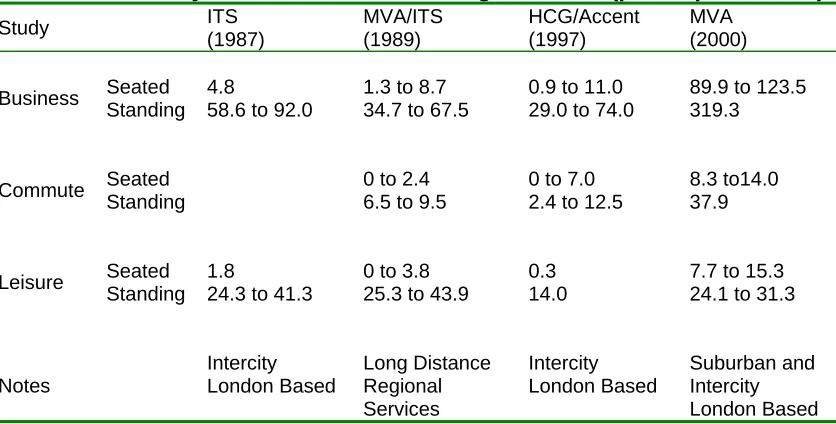
Passengers on crowded or overcrowded trains will typically experience discomfort associated with having to stand or sit in cramped conditions. The level of discomfort varies according to whether the passenger is sitting or standing, the degree of overcrowding, the length of the journey and the type of journey being made (e.g. commuters may be used to overcrowding on short journeys). Much of the published research on passengers’ valuation of overcrowding uses stated preference techniques to assess the trade-off between fares, times and crowding to derive monetary or time estimates of overcrowding penalties. A summary of the findings of this research is presented in Table 1.
INSERT TABLE 1 ABOUT HERE
The penalties vary widely across the studies, but it is clear that those passengers who are left standing through overcrowding suffer much more discomfort than those seated in cramped conditions.
Penalties vary depending on the type of traveller. Commuters, who may be used to overcrowding on short journeys, have the lowest penalties. Business travellers, who may have to work on-board, suffer the highest penalties.
2.2.2 Setting the Scale of the Model
The demand model described in section 2.1 includes a set of scaling coefficients (λ values) which govern the sensitivity of demand to changes in generalised cost. These scales can be set to replicate known fare and GJT elasticities of demand.
The elasticity of demand for ticket type t with respect to the GJT for ticket type
t is given as:
(
)
(
t|r)
t(
tr r | t r GJT
t 1 1 P vot*GJT
1 P P 1 t λ ⎥ ⎦ ⎤ ⎢ ⎣ ⎡ − ⎟⎟ ⎠ ⎞ ⎜⎜ ⎝ ⎛ − λ + − =
η
)
(8)Where is the probability of choosing ticket type t conditional on rail being chosen.
r | t P
The cross elasticity of demand for ticket type s with respect to the generalised journey time for ticket type t is given as:
(
t t r | t r r | t r GJTs 1P vot*GJT
1 P P t λ ⎥ ⎦ ⎤ ⎢ ⎣ ⎡ ⎟⎟ ⎠ ⎞ ⎜⎜ ⎝ ⎛ − λ + − =
η
)
(9)As improvements to generalised journey time will, by and large, impact all ticket types, the GJT elasticities can be thought of as ‘conditional elasticities’ which are expressed as:
Given that we know the base market shares for rail and for each ticket group and that we can estimate a value for GJT for each ticket group, we can set the values of so that the conditional elasticities of demand for each ticket type are equal to those suggested by empirical research.
t
λ
Whilst the conditional GJT elasticities for each ticket type (equation 10) are independent of the nesting parameter λr, the coefficient has important implications for the size of the own (equation 8) and cross (equation 9) elasticities of demand, and to the sensitivity of the model to changes in the size of the choice set (i.e. the addition or withdrawal of choice options). The calibration of is achieved via a trial and error process in which the elasticities of demand to GJT and to fare are set to replicate known values.
r
λ
2.2.3 Replicating the Base Market Shares
Following the estimation of the generalised cost of each option and the calibration of the scaling coefficients, the model is applied to generate forecasts for each operator and ticket type. To ensure that the model is able to correctly forecast ticket market shares in the base period, a full set of model constants are derived using equation 11 and inserted in the generalised cost expression (equation 5).
⎟⎟ ⎠ ⎞ ⎜⎜ ⎝ ⎛ ′ λ − =
t t r base t new
t
P P ln ASC
ASC (11)
Where base t
ASC is the base constant for ticket type t new
t
ASC is the new constant for ticket type t
t
P′ is the forecast share of ticket type t
t
P is the actual share of ticket type t
The alternative specific constants for each ticket type are initially set to zero and the model is then run to generate forecasts of the share of each ticket type. These forecasts are then compared with actual ticket sales data and a new set of model constants derived. These constants capture the impact of the range of factors that influence passengers’ choice of tickets that are not already included within the generalised cost expression.
2.3 Application of the Model to Forecast Demand
The way in which the model is applied is outlined in the step-by-step procedure shown below:
(ii) For each simulated individual, the model estimates the generalised cost of travel for each available ticket type and return-service combination using equation 5, and assigns each travel option a probability that it will be chosen using equation 2.
(iii) The market shares for each service and ticket type are then estimated by averaging the derived probabilities over all simulated individuals.
(iv) To allow for the fact that changing fares and services will change the overall demand for rail, the upper level of the model (equation 4) is structured to allow rail’s market share to expand or contract according to the overall quality of rail, as defined by its composite cost.
(v) The number of individuals using each travel option is then estimated by factoring the relevant market share information (steps iii and iv) by the base period demand, which is defined by the user.
(vi) Using load factors based on number of individuals on a particular service, an overcrowding penalty is calculated for each service. Steps ii to v are then repeated, incorporating the overcrowding penalty for services into the generalised cost calculation of step ii.
3. Case Study
To keep the case study example simple, we have defined a core network of services operating between two regional rail stations in the North of England. In the interest of commercial confidentiality the stations are simply referred to as Station A and Station B.
Table 2 provides a summary of the case study network characteristics. The timetable, fares, ticket restrictions, base demand and market share information were all derived from information kindly supplied by the Strategic Rail Authority. The fare for each ticket type is specified in terms of a return fare equivalent and ‘reduced’ tickets are specified to be unavailable between 0700 and 0900 and between 1600 and 1800. Passenger preferences including the value of time, value of adjustment time and crowding penalties were set to be equal to those recommended in the Passenger Demand Forecasting Handbook (ATOC, 2002) and the GJT elasticities and desired departure time profiles taken to be equal to those used in the commonly used MOIRA rail demand model (AEAT, 2002).
INSERT TABLE 2 ABOUT HERE
INSERT FIGURE 1 ABOUT HERE
Figure 1 shows the demand profiles for traffic between Station A and Station B. As would be expected, the desired departure time shows greater demand in the peaks but this latent demand is ‘priced-off’ by the higher priced tickets. In this instance it appears as though the operator has set the fare differentials between the peak and off-peak and the ticket restrictions at reasonable levels to manage overcrowding although as the assumed capacity of trains was set at 250 seats there are still some problems with overcrowding in the peak periods. A comparison of the forecasts with the guard counts is promising, with forecast demand closely mapping actual demand.
INSERT FIGURE 2 ABOUT HERE
Forecasts of demand profiles for Station B to Station A (Figure 2) are not as encouraging as forecasts for Station A to Station B. This might be expected given that the guard counts are more capricious and there appears to be bigger differences between the assumed desired departure time profile and the guard count data.
To illustrate how demand is allocated between ticket types throughout the day, Figure 3 shows a plot of the demand by ticket type throughout the day. This plot is given for services between Station B and Station A and shows how the imposition of ticketing restrictions influences the distribution of ticket sales.
INSERT FIGURE 3 ABOUT HERE
Following successful calibration and validation, the model was subsequently applied to generate forecasts in a number of scenarios to examine the sensitivity of demand to changes in train seating capacity, ticketing restrictions and fare differentials between ticket types. The focus of the model runs is to examine alternative ways to manage overcrowding. Key model results are presented in Table 3.
INSERT TABLE 3 ABOUT HERE
Widening the peak period ticket restrictions from ‘0700-0900 and 1600-1800’ to ‘0700-0930 and 1530-1800’ reduces the overall demand for travel by 1% but increases operator revenue as demand for full fare tickets increases. Further changes to ticketing restrictions to ‘0630-0930 and 1530-1830’ are forecast to lead to more substantial reductions in demand (2%) and marginal gains in revenue. Peak train loading is largely unaffected by the change to ticket departure time restrictions.
More substantial reductions to train overcrowding can be achieved by increasing the fare differentials between peak and off-peak travel. Increasing the price of full fare tickets by 10% and 30% reduces peak loading from 130% to 126% and 119% respectively. These price changes have substantial impacts on the demand for full fare tickets but as significant proportion of the ‘priced off’ traffic transfers to ‘reduced’ and season tickets the overall impact on demand and revenue is modest. Alternatively, fare differentials between the peak and off-peak can be increased by discounting off-peak fares. Here, discounts of 10% and 30% generate only small reductions in peak load factors at the expense of fairly significant reductions in revenue.
At the current elasticity levels, reductions to off-peak fares generate passenger benefits at the expense of operator losses, and increases to peak fares generate operator gains at the expense of passenger losses. Combining the two strategies allowing for fare increases in the peak and fare reductions in the off-peak generate significant reductions in overcrowding with marginal changes to demand and operator revenue. Under the current regulation, peak fares are regulated to limit fare increases to less than RPI+1%. This policy is aimed at protecting passengers where operators have market power but may restrict the potential of using price discrimination to manage demand levels throughout the day.
4. Conclusions
This paper reports on the development of the PRAISE rail operation model to incorporate the demand response to overcrowding on individual services. The model simulates the choices of individual travellers and assigns a probability that each traveller will choose a given service and ticket combination. The model employs widely used attribute valuations and is calibrated to replicate known aggregate elasticities of demand. The model is applied to data for a regional inter-urban route in the North of England and validated to guard count data to ensure that it can adequately forecast demand at the individual service level.
Acknowledgments
This work was undertaken as part of a project funded by the Strategic Rail Authority. The views expressed in this paper are those of the authors and do not necessarily reflect those of the sponsor.
References
AEAT, 2002. MOIRA, AEA Technology Rail, Derby
ATOC, 2002. Passenger Demand Forecasting Handbook, Association of Train Operating Companies, London
HCG/Accent, 1997. Customer Valuation of Different Load Factors, (Unpublished Report), Accent/Hague Consulting Group, Cambridge,
ITS, 1987. The Values of Overcrowding and Departure Time Variations for InterCity Rail Travellers, Project Report, Institute for Transport Studies, University of Leeds
MVA and ITS, 1989. Regional Railways Overcrowding Study, Undertaken on behalf of Regional Railways, Institute for Transport Studies, University of Leeds
MVA, 2000. Valuations of Crowding Improvements, Unpublished Report to the Strategic Rail Authority, London
Preston, J., Whelan, G.A., and Wardman, M.R., 1999. An Analysis of the Potential for On-track Competition in the British Passenger Rail Industry, Journal of Transport Economics and Policy, 36, (1) 77-94
Wardman, M and Fowkes, A.S., 1987 The Values of Overcrowding and Departure Time Variations for Intercity Rail Travellers, Institute for Transport Studies, University of Leeds, ITS Technical Note 229
Whelan, G.A., Preston, J.M., Wardman, M., and Nash, C.A., 1997. The Privatisation of Passenger Rail Services in Britain: An Assessment of the Impacts of On-the-track Competition, Presented to European Transport Forum, PTRC 1997
0 100 200 300 400 500
0 2 4 6 8 10 12 14 16 18 20 22 24 Time
Demand
Guard Count Desired Departure Profile Estimate
0 100 200 300 400 500 600
0 2 4 6 8 10 12 14 16 18 20 22 24
Time
Demand
Count Estimate Desired Departure Profile
0 20 40 60 80 100 120 140 160 180
0 2 4 6 8 10 12 14 16 18 20 22 24 Time
Demand (Return Trips)
[image:16.595.96.475.94.321.2]Full Reduced Season All
Table 1: Summary Review of Overcrowding Penalties (pence per minute)
Study ITS
(1987)
MVA/ITS (1989)
HCG/Accent (1997)
MVA (2000)
Seated 4.8 1.3 to 8.7 0.9 to 11.0 89.9 to 123.5
Business
Standing 58.6 to 92.0 34.7 to 67.5 29.0 to 74.0 319.3
Seated 0 to 2.4 0 to 7.0 8.3 to14.0
Commute
Standing 6.5 to 9.5 2.4 to 12.5 37.9
Seated 1.8 0 to 3.8 0.3 7.7 to 15.3
Leisure
Standing 24.3 to 41.3 25.3 to 43.9 14.0 24.1 to 31.3
Notes
Intercity London Based
Long Distance Regional Services
Intercity London Based
Table 2: Network Characteristics and Modelling Assumptions
Full £4.55
Reduced £3.20
Return Fare
Season £3.30
Full 60%
Reduced 37%
Shares
Season 3%
Number per day 46
Services
Core Frequency 3 service per hour
Journey Time 25 minutes
Demand (return Trips per day) 5132
Full -0.58
Reduced -0.56
GJT Elasticity
Season -0.60
Overall Fare Elasticity -0.41
Value of Time (pence per minute) 5.0
Value of Adjustment Time (pence per minute) 2.5
Table 3: Key Scenario Results
Policy Demand Peak
Seats Restrictions Fares Full Reduced Season Total Revenue Loading
As now
Restrict 1 As now 3,141
1,867 124 5,132
20,675
130%
-10% Restrict 1 As now 2,990
(95%) 1,788 (96%) 114 (92%) 4,891 (95%) 19,698
(95%) 138%
-30% Restrict 1 As now 2,729
(87%) 1,648 (88%) 96 (78%) 4,473 (87%) 18,009
(87%) 174%
As
now Restrict 2 As now
3,425 (109%) 1,510 (81%) 136 (109%) 5,071 (99%) 20,866
(101%) 129%
As
now Restrict 3 As now
3,555 (113%) 1,346 (72%) 141 (114%) 5,042 (98%) 20,947
(101%) 128%
As
now Restrict 1 +10% Full
2,813 (90%) 1,987 (106%) 188 (151%) 4,987 (97%) 21,039
(102%) 126%
As
now Restrict 1 +30% Full
2,192 (70%) 2,123 (114%) 428 (345%) 4,743 (92%) 21,182
(102%) 119%
As
now Restrict 1 -10% Reduced
3,054 (97%) 2,025 (108%) 120 (97%) 5,199 (101%) 20,124
(97%) 129%
As
now Restrict 1 -30% Reduced
2,933 (93%) 2,303 (123%) 115 (93%) 5,351 (104%) 18,883
(91%) 127%
As
now Restrict 3
+30% Full -30% Reduced 2,563 (82%) 1,706 (91%) 502 (405%) 4,771 (93%) 20,651
(100%) 121%
Notes:
Demand is shown as return trips per day with percent of base demand shown in brackets Revenue is shown as £s per day with percent of base revenue shown in brackets
Peak loading shows the highest train loading throughout the day