Causality, Influence, and Computation in Possibly Disconnected
Synchronous Dynamic Networks
I,IIOthon Michaila,∗, Ioannis Chatzigiannakisa, Paul G. Spirakisa,b
aComputer Technology Institute & Press “Diophantus” (CTI), Patras, Greece bDepartment of Computer Science, University of Liverpool, UK
Abstract
In this work, we study the propagation of influence and computation in dynamic distributed computing systems that are possibly disconnected at every instant. We focus on asynchronous message passing commu-nication model with broadcast and bidirectional links. Our network dynamicity assumption is aworst-case dynamicity controlled by an adversary scheduler, which has received much attention recently. We replace the usual (in worst-case dynamic networks) assumption that the network is connected at every instant by minimaltemporal connectivity conditions. Our conditions only require thatanother causal influence occurs within every time-window of some given length. Based on this basic idea we define several novel metrics for capturing the speed of information spreading in a dynamic network. We present several results that correlate these metrics. Moreover, we investigatetermination criteriain networks in which an upper bound on any of these metrics is known. We exploit our termination criteria to provide efficient (and optimal in some cases) protocols that solve the fundamentalcounting andall-to-all token dissemination (orgossip) problems.
Keywords:
dynamic graph, mobile computing, worst-case dynamicity, adversarial schedule, temporal connectivity, termination, counting, information dissemination, optimal protocol
1. Introduction
Distributed computing systems are more and more becoming dynamic. The static and relatively stable models of computation can no longer represent the plethora of recently established and rapidly emerging information and communication technologies. In recent years, we have seen a tremendous increase in the number of new mobile computing devices. Most of these devices are equipped with some sort of communi-cation, sensing, and mobility capabilities. Even the Internet has become mobile. The design is now focused on complex collections of heterogeneous devices that should be robust, adaptive, and self-organizing, possi-bly moving around and serving requests that vary with time. Delay-tolerant networks are highly-dynamic, infrastructure-less networks whose essential characteristic is a possible absence of end-to-end communication routes at any instant. Mobility may be active, when the devices control and plan their mobility pattern (e.g. mobile robots), orpassive, in opportunistic-mobility networks, where mobility stems from the mobility of the carries of the devices (e.g. humans carrying cell phones) or a combination of both (e.g. the devices
ISupported in part by the project “Foundations of Dynamic Distributed Computing Systems” (FOCUS) which is implemented under the “ARISTEIA” Action of the Operational Programme “Education and Lifelong Learning” and is co-funded by the European Union (European Social Fund) and Greek National Resources.
IIA preliminary version of the results in this paper has appeared in [MCS12b].
∗Corresponding author (Telephone number: +30 2610 960200, Fax number: +30 2610 960490, Postal Address: Computer
Technology Institute & Press “Diophantus” (CTI), N. Kazantzaki Str., Patras University Campus, Rio, P.O. Box 1382, 26504, Greece).
have partial control over the mobility pattern, like for example when GPS devices provide route instructions to their carriers). Thus, it can vary from being completely predictable to being completely unpredictable. Gossip-based communication mechanisms, e-mail exchanges, peer-to-peer networks, and many other contem-porary communication networks all assume or induce some sort of highly-dynamic communication network. The formal study of dynamic communication networks is hardly a new area of research. There is a huge amount of work in distributed computing that deals with causes of dynamicity such as failures and changes in the topology that are rather slow and usually eventually stabilize (like, for example, in self-stabilizing systems [Dol00]). However the low rate of topological changes that is usually assumed there is unsuitable for reasoning about truly dynamic networks. Even graph-theoretic techniques need to be revisited: the suitable graph model is now that of adynamic graph (a.k.a. temporal graph or time-varying graph) (see e.g. [MMCS13, KKK00, CFQS12]), in which each edge has an associated set of time-labels indicating availability times. Even fundamental properties of classical graphs do not easily carry over to their temporal counterparts. For example, Kempe, Kleinberg, and Kumar [KKK00] found out that there is no analogue of Menger’s theorem (see e.g. [Bol98] for a definition) for arbitrary temporal networks with one label on every edge, which additionally renders the computation of the number of node-disjoint s-t paths
NP-complete. Very recently, the authors of [MMCS13] achieved a reformulation of Menger’s theorem which is valid for all temporal networks and additionally they introduced several interesting cost minimization parameters for optimal temporal network design and gave some first results on them. Even the standard network diameter metric is no more suitable and has to be replaced by a dynamic/temporal version. In a dynamic star graph in which all leaf-nodes but one go to the center one after the other in a modular way, any message from the node that enters last the center to the node that never enters the center needsn−1 steps to be delivered, wherenis the size (number of nodes) of the network; that is thedynamic diameter is
n−1 while, one the other hand, the classical diameter is just 2 [AKL08] (see also [KO11]).
2. Related Work
Distributed systems with worst-case dynamicity were first studied in [OW05]. Their outstanding novelty was to assume a communication network that may change arbitrarily from time to time subject to the condition that each instance of the network is connected. They studied asynchronous communication and considered nodes that can detect local neighborhood changes; these changes cannot happen faster than it takes for a message to transmit. They studiedflooding (in which one node wants to disseminate one piece of information to all nodes) androuting(in which the information need only reach a particular destination node
t) in this setting. They described a uniform protocol for flooding that terminates in O(T n2) rounds using O(logn) bit storage and message overhead, where T is the maximum time it takes to transmit a message. They conjectured that without identifiers (IDs) flooding is impossible to solve within the above resources. Finally, a uniform routing algorithm was provided that delivers to the destination in O(T n) rounds using
O(logn) bit storage and message overhead.
Computation under worst-case dynamicity was further and extensively studied in a series of works by Kuhn et al. in the synchronous case. In [KLO10], the network was assumed to be T-interval connected meaning that any time-window of lengthT has a static connected spanning subgraph (persisting throughout the window). Among others,counting (in which nodes must determine the size of the network) andall-to-all token dissemination (in whichndifferent pieces of information, called tokens, are handed out to thennodes of the network, each node being assigned one token, and all nodes must collect all n tokens) were solved in O(n2/T) rounds using O(logn) bits per message, almost-linear-time randomized approximate counting
distributed computation under worst-case dynamicity see [KO11]. Two very thorough surveys on dynamic networks are [Sch02, CFQS12].
Another notable model for dynamic distributed computing systems is the population protocol model [AAD+06]. In that model, the computational agents are passively mobile, interact in ordered pairs, and the
connectivity assumption is astrong global fairness condition according to which all events that may always occur, occur infinitely often. These assumptions give rise to some sort of structureless interacting automata model. The usually assumed anonymity and uniformity (i.e. n is not known) of protocols only allow for commutative computations that eventually stabilize to a desired configuration. Most computability issues in this area have now been established. Constant-state nodes on a complete interaction network (and several variations) compute the semilinear predicates [AAER07]. Semilinearity persists up to o(log logn) local space but not more than this [CMN+11]. If constant-state nodes can additionally leave and update
fixed-length pairwise marks then the computational power dramatically increases to the commutative subclass of
NSPACE(n2) [MCS11a]. For a very recent introductory text see [MCS11b].
3. Contribution
In this work, we study worst-case dynamic networks that arefree of any connectivity assumption about their instances. Our dynamic network model is formally defined in Section 4.1. We only impose sometemporal connectivityconditions on the adversary guaranteeing thatanother causal influence occurs within every time-window of some given length, meaning that, in that time, another node first hears of the state that some node
uhad at some timet (see Section 4.3 for a formal definition of causal influence). Note that our temporal connectivity conditions are minimal assumptions that allow for bounded end-to-end communication in any dynamic network including those that have disconnected instances. Based on this basic idea, we define several novel generic metrics for capturing the speed of information spreading in a dynamic network. In particular, we define theoutgoing influence time (oit) as the maximal time until the state of a nodeinfluences the state of another node, theincoming influence time(iit) as the maximal time until the state of a nodeis influenced by the state of another node, and the connectivity time(ct) as the maximal time until the two parts of any cut of the network become connected. These metrics are defined in Section 5, where also several results that correlate these metrics to themselves and to standard metrics, like e.g. the dynamic diameter, are presented. In Section 5.1, we present a simple but very fundamental dynamic graph based on alternating matchings that hasoit 1 (equal to that of instantaneous connectivity networks) but at the same time isdisconnected in every instance. In Section 6, we exhibit another dynamic graph additionally guaranteeing that edges take maximal time to reappear. That graph is based on a geometric edge-coloring method due to Soifer for coloring a complete graph of even order n with n−1 colors [Soi09]. Similar results have appeared before but to the best of our knowledge only in probabilistic settings [CMM+08, BCF09].
In Section 7, we turn our attention to terminating computations and, in particular, we investigate termi-nation criteria in networks in which an upper bound on thector theoitis known. By “termination criterion” we essentially mean any locally verifiable property that can be used to determine whether a node has heard from all other nodes. Note that we do not allow to the nodes any further knowledge on the network; for instance, nodesdo not know the dynamic diameter of the network. In particular, in Section 7.1, we study the case in which an upper boundT on thectis known and we present an optimal termination criterion that only needs time linear in the dynamic diameter and inT. Then, in Section 7.2, we study the case in which an upper boundKon theoitis known. We first present a termination criterion that needs timeO(K·n2).
Additionally, we establish that the optimal termination criterion for thectcase does not work in theoitcase. These criteria share the fundamental property of “hearing from the past”. We then develop a new technique that gives an optimal termination criterion (time linear in the dynamic diameter and inK) by “hearing from the future” (by this we essentially mean that a node is interested for its outgoing influences instead for its incoming ones). Additionally, we exploit throughout the paper our termination criteria to provide protocols that solve the fundamentalcounting andall-to-all token dissemination (or gossip) problems; in the former nodes must determine the size of the networknand in the latter each node of the network is provided with a unique piece of information, calledtoken, and all nodes must collect allntokens.
4. Preliminaries
4.1. The Dynamic Network Model
Adynamic networkis modeled by adynamic graphG= (V, E), whereV is a set ofnnodes (or processors) and E: N→ P(E0) (wherever we useN we meanN≥1) is a function mapping a round numberr ∈Nto a set E(r) of bidirectional links drawn from E0 =
{{u, v} : u, v ∈ V}. 1 Intuitively, a dynamic graphG is
an infinite sequenceG(1), G(2), . . .of instantaneous graphs, whose edge sets are subsets ofE0 chosen by a worst-case adversary. Astatic network is just a special case of a dynamic network in whichE(i+ 1) =E(i) for alli∈N. The setV is assumed throughout this work to bestatic, that is it remains the same throughout the execution.
We assume that nodes inV have unique identities (ids) drawn from some namespaceU (we assume that ids are represented usingO(logn) bits) and that they do not know the topology or the size of the network, apart from some minimal necessary knowledge to allow for terminating computations (usually an upper bound on the time it takes for information to make some sort of progress). Any such assumed knowledge will be clearly stated. Moreover, nodes have unlimited local storage (though they usually use a reasonable portion of it).
Communication issynchronous message passing [Lyn96, AW04], meaning that it is executed in discrete steps controlled by a global clock that is available to the nodes and that nodes communicate by sending and receiving messages (usually of length that is some reasonable function ofn, like e.g. logn). We use the terms round, time, and step interchangeably to refer to the discrete steps of the system. Naturally, real rounds begin to count from 1 (e.g. “first round”) and we reserve time 0 to refer to the initial state of the system. We assume that the message transmission model isanonymous broadcast, in which, in every roundr, each node
ugenerates a single messagemu(r) to be delivered to all its current neighbors inNu(r) ={v:{u, v} ∈E(r)} without knowingNu(r).
In every round, the adversary first chooses the edges for the round; for this choice it can see the internal states of the nodes at the beginning of the round. At the same time and independently of the adversary’s choice of edges each node generates its message for the current round. Note that a node does not have any information about the internal state of its neighbors when generating its messages (including their ids). In deterministic algorithms, nodes are only based on their current internal state to generate their messages and this implies that the adversary can infer the messages that will be generated in the current round before choosing the edges. In this work, we only consider deterministic algorithms. Each message is then delivered to the sender’s neighbors, as chosen by the adversary; the nodes transition to new states, and the next round begins.
4.2. Problem Definitions
In this work, apart from studying the structural properties of possibly disconnected dynamic networks we also investigate the computability of the following two fundamental problems for distributed computing.
Counting. Nodes must determine the network size n.
All-to-all Token Dissemination (or Gossip). There is a token assignment function I : V → T that assigns to each node u∈ V a single token I(u) from some domain T s.t. I(u) 6= I(v) for all u 6=v. An algorithm solves all-to-all token dissemination if for all instances (V, I), when the algorithm is executed in any dynamic graphG= (V, E), all nodes eventually terminate and outputS
u∈V I(u). We assume that each token in the nodes’ input is represented usingO(logn) bits. The nodes know that each node starts with a unique token but they do not known.
4.3. Spread of Influence in Dynamic Graphs (Causal Influence)
Probably the most important notion associated with a dynamic network/graph is the causal influence, which formalizes the notion of one node “influencing” another through a chain of messages originating at the former node and ending at the latter (possibly going through other nodes in between). We denote by (u, t) the state of nodeuat timet and usually call it thet-state of u. The pair (u, t) is also called atime-node. We use (u, r) (v, r0) to denote the fact that node u’s state in round r influences nodev’s state in round
r0. Formally:
Definition 1 ([Lam78]). Given a dynamic graphG = (V, E) we define an order →⊆(V ×N≥0)2, where
(u, r) →(v, r+ 1) iffu =v or {u, v} ∈ E(r+ 1). The causal order ⊆ (V ×N≥0)2 is defined to be the
reflexive and transitive closure of→.
Obviously, for a dynamic distributed system to operate as a whole there must exist some upper bound on the time needed for information to spread through the network. This is a very weak guarantee as without it global computation is in principle impossible. An abstract way to talk about information spreading is via the notion of the dynamic diameter. Thedynamic diameter (also called flooding time, e.g., in [CMM+08,
BCF09]) of a dynamic graph, is an upper bound on the time required for each node to causally influence (or, equivalently, to be causally influenced by) every other node; formally, the dynamic diameter is the minimum
D ∈N s.t. for all timest≥0 and all u, v∈V it holds that (u, t) (v, t+D). A small dynamic diameter allows for fast dissemination of information. In this work, we do not allow nodes to know the dynamic diameter of the network. We only allow some minimal knowledge (that will be explained in the sequel) based on which nodes may infer bounds on the dynamic diameter.
A class of dynamic graphs with small dynamic diameter is that of T-interval connected graphs. T -interval connectivity was proposed in [KLO10] as an elegant way to capture a special class of dynamic networks, namely those that are connected at every instant. Intuitively, the parameter T represents the rate of connectivity changes. Formally, a dynamic graph G = (V, E) is said to be T-interval connected, for T ≥ 1, if, for all r ∈ N, the static graph Gr,T := (V,T
r+T−1
i=r E(r)) is connected [KLO10]; that is, in every time-window of lengthT, a connected spanning subgraph is preserved. In one extreme, ifT = 1 then the underlying connected spanning subgraph may change arbitrarily from round to round and in the other extreme ifT is∞then a connected spanning subgraph must be preserved forever.
T-interval connected networks have the very nice feature to allow for constant propagation of information. For example, 1-interval connectivity guarantees that the state of a node causally influences the state of another uninfluenced node in every round (if one exists). To get an intuitive feeling of this fact, consider a partitioning of the set of nodes V to a subset V1 of nodes that know the r-state of some node u and to a subsetV2=V\V1of nodes that do not know it. Connectivity asserts that there is always an edge in the cut betweenV1 and V2, consequently, if nodes that know ther-state of ubroadcast it in every round, then in every round at least one node moves fromV2 toV1.
This is formally captured by the following lemma from [KLO10].
Lemma 1([KLO10]). For any node u∈V and timer≥0, in a 1-interval connected network, we have
1. |{v∈V : (u,0) (v, r)}| ≥min{r+ 1, n}, 2. |{v∈V : (v,0) (u, r)}| ≥min{r+ 1, n}.
Let us also define two very useful sets. For all times 0 ≤t ≤t0, we define by past
(u,t0)(t) :={v ∈V : (v, t) (u, t0)
} [KMO11] thepast set of a time-node (u, t0) from time t and by future
(u,t)(t0) :={v ∈V :
(u, t) (v, t0)
}thefuture set of a time-node(u, t)at timet0. In words, past
(u,t0)(t) is the set of nodes whose
t-state (i.e. their state at timet) has causally influenced thet0-state ofuand future
(u,t)(t0) is the set of nodes
whose t0-state has been causally influenced by the t-state of u. If v∈ future
(u,t)(t0) we say that at timet0
nodev has heard of/from thet-state of nodeu. If it happens thatt= 0 we say simply thatv has heard of
u. Note thatv∈past(u,t0)(t) iffu∈future(v,t)(t0).
For a distributed system to be able to perform global computation, nodes need to be able to determine for all times 0 ≤t ≤t0 whether past
timet0 whether past
(u,t0)(t) =V by counting all differentt-states that it has heard of so far (provided that every node broadcasts at every round all information it knows). If it has heard thet-states of all nodes then the equality is satisfied. Ifnis not known then various techniques may be applied (which is the subject of this work). Bytermination criterion we mean any locally verifiable property that can be used to determine whether past(u,t0)(t) =V.
Remark 1. Note that any protocol that allows nodes to determine whether past(u,t0)(t) =V can be used to solve the counting and all-to-all token dissemination problems. The reason is that if a node knows at round
r that it has been causally influenced by the initial states of all other nodes, then it can solve counting by writing|past(u,r)(0)|on its output and all-to-all dissemination by writingpast(u,r)(0)(provided that all nodes
send their initial states and all nodes constantly broadcast all initial states that they have heard of so far).
5. Our Metrics
As already stated, in this work we aim to deal with dynamic networks that are allowed to have dis-connected instances. To this end, we define some novel generic metrics that are particularly suitable for capturing the speed of information propagation in such networks.
5.1. The Influence Time
Recall that the guarantee on propagation of information resulting from instantaneous connectivity ensures that any time-node (u, t) influences another node in each step (if an uninfluenced one exists). From this fact, we extract two novel generic influence metrics that capture the maximal time until another influence (outgoing or incoming) of a time-node occurs.
We now formalize our first influence metric.
Definition 2(Outgoing Influence Time). We define the outgoing influence time (oit) as the minimumk∈N s.t. for allu∈V and all times t, t0
≥0 s.t. t0
≥t it holds that
|future(u,t)(t0+k)| ≥min{|future(u,t)(t0)|+ 1, n}.
Intuitively, theoitis the maximal time until thet-state of a node influences the state of another node (if an uninfluenced one exists) and captures the speed of information spreading.
Our second metric is similarly defined as follows.
Definition 3(Incoming Influence Time). We define theincoming influence time(iit) as the minimumk∈N s.t. for allu∈V and all times t, t0≥0 s.t. t0≥t it holds that
|past(u,t0+k)(t)| ≥min{|past(u,t0)(t)|+ 1, n}.
We can now say that the oit of a T-interval connected graph is 1 and that the iitcan be up to n−2. However, is it necessary for a dynamic graph to beT-interval connected in order to achieve unitoit? First, let us make a simple but useful observation:
Proposition 1. If a dynamic graph G = (V, E) has oit (or iit) 1 then every instance has at least dn/2e edges.
Proof. ∀u∈V and ∀t≥1 it must hold that {u, v} ∈E(t) for some v. In words, at any time t each node must have at least one neighbor since otherwise it influences (or is influenced by) no node during roundt. A minimal way to achieve this is by a perfect matching in the even-order case and by a matching between
n−3 nodes and a linear graph between the remaining 3 nodes in the odd-order case.
Proposition 1 is easily generalized as: if a dynamic graphG= (V, E) hasoit(oriit)kthen for all timest
it holds that|St+k−1
Now, inspired by Proposition 1, we define a minimal dynamic graph that at the same time satisfiesoit 1 and always disconnected instances:
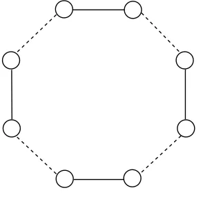
[image:7.612.233.380.155.298.2]The Alternating Matchings Dynamic Graph. Take a ring of an even number of nodesn= 2l, partition the edges into 2 disjoint perfect matchings Aand B (each consisting ofl edges) and alternate round after round between the edge setsAandB (see Figure 1).
Figure 1: The Alternating Matchings dynamic graph forn= 8. The solid lines appear every odd round (1,3,5, . . .) while the dashed lines every even round (2,4,6, . . .).
Proposition 2. The Alternating Matchings dynamic graph hasoit1 and any node needs preciselyn/2rounds to influence all other nodes.
Proof. Take any nodeu. In the first round, uinfluences its left or its right neighbor on the ring depending on which of its two adjacent edges becomes available first. Thus, including itself, it has influenced 2 nodes forming a line of length 1. In the next round, the two edges that join the endpoints of the line with the rest of the ring become available and two more nodes become influenced; the one is the neighbor on the left of the line and the other is the neighbor on the right. By induction on the number of rounds, it is not hard to see that the existing line always expands from its endpoints to the two neighboring nodes of the ring (one on the left and the other on the right). Thus, we get exactly 2 new influences per round, which gives oit 1 andn/2 rounds to influence all nodes.
In the alternating matchings construction any edge reappears every second step but not faster than this. We now formalize the notion of thefastest edge reappearance (fer) of a dynamic graph.
Definition 4. Thefastest edge reappearance(fer) of a dynamic graphG= (V, E)is defined as the minimum
p∈Ns.t.,∃e∈ {{u, v}:u, v ∈V} and∃t∈N,e∈E(t)∩E(t+p).
Clearly, the fer of the alternating matchings dynamic graph described above is 2, because no edge ever reappears in 1 step and some, at some point, (in fact, all and always) reappears in 2 steps. In Section 6, by invoking a geometric edge-coloring method, we generalize this basic construction to a more involved dynamic graph withoit 1, always disconnected instances, andferequal ton−1. 2
We next give a proposition associating dynamic graphs withoit(oriit) upper bounded byK to dynamic graphs with connected instances.
Proposition 3. Assume that the oit or the iit of a dynamic graph, G = (V, E), is upper bounded by K. Then for all timest∈Nthe graph (V,Sit=+tKbn/2c−1E(i))is connected.
2It is interesting to note that in dynamic graphs with a static set of nodes (that isV does not change), if at least one change
happens each time, then every instanceG(t) will eventually reappear after at mostP n
2
k=0 n
2
k
Proof. It suffices to show that for any partitioning (V1, V2) of V there is an edge in the cut labeled from {t, . . . , t+Kbn/2c−1}. W.l.o.g. letV1be the smaller one, thus|V1| ≤ bn/2c. Take anyu∈V1. By definition of oit,|future(u,t)(t+Kbn/2c −1)| ≥ |future(u,t)(t+K|V1| −1)| ≥ |V1|+ 1 implying that some edge in the
cut has transferredu’st-state out ofV1 at some time in the interval [t, t+Kbn/2c −1]. The proof for the
iitis similar.
5.2. The Moi (Concurrent Progress)
Consider now the following influence metric:
Definition 5. Define themaximum outgoing influence(moi) of a dynamic graphG= (V, E)as the maximum
k for which∃u∈V and∃t, t0∈
N,t0 ≥t, s.t.|future(u,t)(t0+ 1)| − |future(u,t)(t0)|=k.
In words, the moi of a dynamic graph is the maximum number of nodes that are ever concurrently influenced by a time-node.
Here we show that one cannot guarantee at the same time unit oit and at most one outgoing influence per node per step. In fact, we conjecture that unitoitimplies that some node disseminates inbn/2csteps.
We now prove an interesting theorem stating that if one tries to guarantee unit oit then she must necessarily accept that at some steps more than one outgoing influences of the same time-node will occur leading to faster dissemination thann−1 for this particular node.
Theorem 1. Themoi of any dynamic graph withn≥3 and unitoit is at least 2.
Proof. Forn= 3, just notice that unitoitimplies that, at any timet, some node has necessarily 2 neighbors. We therefore focus onn≥4. For the sake of contradiction, assume that the statement is not true. Then at any timet any nodeuis connected to exactly one other node v (at least one neighbor is required foroit 1 - see Proposition 1 - and at most one is implied by our assumption). Unit oit implies that, at time t+ 1, at least one ofu, v must be connected to somew∈V\{u, v}, let it be v. Proposition 1 requires that alsou
must have an edge labeledt+ 1 incident to it. If that edge arrives atv, then vhas 2 edges labeledt+ 1. If it arrives atw, thenwhas 2 edges labeledt+ 1. So it must arrive at somez∈V\{u, v, w}. Note now that, in this case, the (t−1)-state ofufirst influences bothw, zat timet+ 1 which is contradictory, consequently themoimust be at least 2.
In fact, notice that the above theorem proves something stronger: Every second step at least half of the nodes influence at least 2 new nodes each. This, together with the fact that it seems to hold for some basic cases, makes us suspect that the following conjecture might be true:
Conjecture 1. If the oitof a dynamic graph is 1then ∀t∈N,∃u∈V s.t.|future(u,t)(t+bn/2c)|=n.
That is, if theoitis 1 then, in everybn/2c-window, some node influences all other nodes (e.g. influencing 2 new nodes per step).
5.3. The Connectivity Time
We now propose another natural and practical metric for capturing the temporal connectivity of a possibly disconnected dynamic network that we call theconnectivity time (ct).
Definition 6(Connectivity Time). We define the connectivity time (ct) of a dynamic network G= (V, E) as the minimum k∈Ns.t. for all timest∈Nthe static graph(V,Sit+=k−t 1E(i))is connected.
Section 5.1. Draw a line that crosses two edges belonging to matchingApartitioning the ring into two parts. Clearly, these two parts communicate every second round (as they only communicate when matching A
becomes available), thus thectis 2 and every instance is disconnected. We now provide a result associating thectof a dynamic graph with itsoit.
Proposition 4. (i)oit≤ct but (ii) there is a dynamic graph withoit 1 andct= Ω(n).
Proof. (i) We show that for allu∈V and all times t, t0
∈N s.t.t0 ≥t it holds that |future(u,t)(t0+ct)| ≥
min{|future(u,t)(t0)|+ 1, n}. AssumeV\future(u,t)(t0)6=∅(as the other case is trivial). In at mostctrounds
at least one edge joins future(u,t)(t0) toV\future(u,t)(t0). Thus, in at mostctrounds future(u,t)(t0) increases
by at least one.
(ii) Recall the alternating matchings on a ring dynamic graph from Section 5.1. Now take any set V of a number of nodes that is a multiple of 4 (this is just for simplicity and is not necessary) and partition it into two sets V1, V2 s.t. |V1|=|V2|=n/2. If each part is an alternating matchings graph for |V1|/2 rounds then every usay inV1 influences 2 new nodes in each round and similarly for V2. Clearly we can keep V1
disconnected fromV2 forn/4 rounds without violatingoit= 1.
The following is a comparison of thectof a dynamic graph with its dynamic diameter D.
Proposition 5. ct≤D≤(n−1)ct.
Proof. ct≤Dfollows from the fact that in time equal to the dynamic diameter every node causally influences every other node and thus, in that time, there must have been an edge in every cut (if not, then the two partitions forming the cut could not have communicated with one another). D≤(n−1)ctholds as follows. Take any nodeuand add it to a setS. Inctroundsuinfluences some node fromV\S which is then added to S. In (n−1)ctrounds S must have become equal to V, thus this amount of time is sufficient for every node to influence every other node. Finally, we point out that these bounds cannot be improved in general as for each ofct=DandD= (n−1)ctthere is a dynamic graph realizing it. ct=Dis given by the dynamic graph that has no edge forct−1 rounds and then becomes the complete graph whileD= (n−1)ctis given by a line in which every edge appears at timesct,2ct,3ct, . . ..
Note that the ctmetric has been defined as an underapproximation of the dynamic diameter. Its main advantage is that it is much easier to compute than the dynamic diameter since it is defined on the union of the footprints and not on the dynamic adjacency itself.
6. Fast Propagation of Information Under Continuous Disconnectivity
In Section 5.1, we presented a simple example of an always-disconnected dynamic graph, namely, the alternating matchings dynamic graph, with optimaloit (i.e. unitoit). Note that the alternating matchings dynamic graph may be conceived as simple as it has small fer (equal to 2). We pose now an interesting question: Is there an always-disconnected dynamic graph with unitoit and fer as big asn−1? Note that this is harder to achieve as it allows of no edge to ever reappear in less thann−1 steps. Here, by invoking a geometric edge-coloring method, we arrive at an always-disconnected graph with unit oit and maximalfer; in particular, no edge reappears in less thann−1 steps.
To answer the above question, we define a very useful dynamic graph coming from the area of edge-coloring.
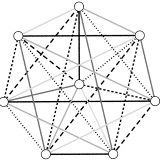
Definition 7. We define the following dynamic graph S based on an edge-coloring method due to Soifer [Soi09]: V(S) = {u1, u2, . . . , un} where n = 2l, l ≥ 2. Place un on the center and u1, . . . , un−1 on the
vertices of a (n−1)-sided polygon. For each time t ≥ 1 make available only the edges {un, umt(0)} for
mt(j) := (t−1 +jmodn−1) + 1 and{umt(−i), umt(i)} fori= 1, . . . , n/2−1; that is make available one
edge joining the center to a polygon-vertex and all edges perpendicular to it. (e.g. see Figure 2 forn= 8and
Figure 2: Soifer’s dynamic graph forn= 8 andt= 1, . . . ,7. In particular, in round 1 the graph consists of the black solid edges, then in round 2 the center becomes connected via a dotted edge to the next peripheral node clockwise and all edges perpendicular to it (the remaining dotted ones) become available, and so on, always moving clockwise.
In Soifer’s dynamic graph, denote byNu(t) :=i:{u, ui} ∈E(t), that is the index of the unique neighbor of uat time t. The following lemma states that the next neighbor of a node is in almost all cases (apart from some trivial ones) the one that lies two positions clockwise from its current neighbor.
Lemma 2. For all times t∈ {1,2, . . . , n−2} and alluk,k∈ {1,2, . . . , n−1}it holds thatNuk(t+ 1) =n
if Nuk(t) = (k−3 modn−1) + 1elseNuk(t+ 1) = (k+ 1 modn−1) + 1 ifNuk(t) =n andNuk(t+ 1) =
(Nuk(t) + 1 modn−1) + 1otherwise.
Proof. Sincek /∈ {n, t, t+ 1} it easily follows thatk, Nk(t), Nk(t+ 1)6=nthus bothNk(t) andNk(t+ 1) are determined by{umt(−i), umt(i)}wheremt(j) := (t−1 +jmodn−1) + 1 andk=mt(−i). The latter implies
(t−1−imodn−1)+1 =k⇒(t−1+imodn−1)+1+(−2imodn−1) =k⇒mt(i) =k−(−2imodn−1); thus, Nk(t) = k−(−2imodn−1). Now let us see how thei that corresponds to some node changes as t
increases. Whentincreases by 1, we have that (t−1 +imodn−1) + 1 = (t+i0modn−1) + 1⇒i0=i−1, i.e. as t increases i decreases. Consequently, for t+ 1 we have Nk(t+ 1) = k−[−2(i−1) modn−1] = (Nuk(t) + 1 modn−1) + 1.
Theorem 2. For all n = 2l, l ≥2, there is a dynamic graph of order n, with oit equal to 1, fer equal to
n−1, and in which every instance is a perfect matching.
Proof. The dynamic graph is the one of Definition 7. It is straightforward to observe that every instance is a perfect matching. We prove now that theoitof this dynamic graph is 1. We focus on the set future(un,0)(t),
that is the outgoing influence of the initial state of the node at the center. Note that symmetry guarantees that the same holds for all time-nodes (it can be verified that any node can be moved to the center without altering the graph). unat time 1 meetsu1and thus future(un,0)(1) ={u1}. Then, at time 2,unmeetsu2and,
by Lemma 2,u1 meetsu3 via the edge than is perpendicular to{un, u2}, thus future(un,0)(2) ={u1, u2, u3}.
We show that for all times t it holds that future(un,0)(t) = {u1, . . . , u2t−1}. The base case is true since
future(un,0)(1) = {u1}. It is not hard to see that, fort ≥2, Nu2(t) = 2t−2,Nu1(t) = 2t−1, and for all ui∈future(un,0)(t)\{u1, u2}, 1≤Nui(t)≤2t−2. Now consider timet+ 1. Lemma 2 guarantees now that
for allui∈future(un,0)(t) we have thatNui(t+ 1) =Nui(t) + 2. Thus, the only new influences at stept+ 1
are byu1 andu2implying that future(un,0)(t+ 1) ={u1, . . . , u2(t+1)−1}. Consequently, theoitis 1.
Note that Theorem 2 is optimal w.r.t. feras it is impossible to achieve at the same time unitoit andfer
strictly greater thann−1. To see this, notice that if no edge is allowed to reappear in less thannsteps then any node must have no neighbors once everynsteps.
7. Termination and Computation
We now turn our attention to termination criteria that we exploit to solve the fundamental counting and all-to-all token dissemination problems. First observe that if nodes know an upper bound H on theiit
then there is a straightforward optimal termination criterion taking timeD+H, whereD is the dynamic diameter. In every round, all nodes forward all ids that they have heard of so far. If a node does not hear of a new id for H rounds then it must have already heard from all nodes. We begin this section by assuming that nodes know an upper bound on thectand show how this initial knowledge can be exploited for optimal termination. Then, we allow the nodes to know an upper bound on the oit. In this case, things turn out to be much harder. We give a termination criterion which, though being far from the dynamic diameter, is optimal if a node terminates based on its past set. We then develop a novel technique that gives an optimal termination criterion based on the future set of a node. Keep in mind that nodes have noa priori knowledge of the size of the network.
7.1. Nodes Know an Upper Bound on thect: An Optimal Termination Criterion
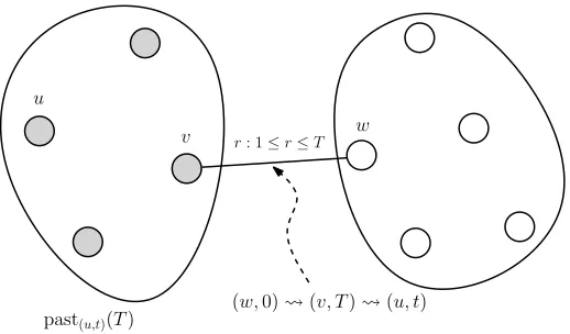
We here assume that all nodes know some upper boundT on thect. We will give an optimal condition that allows a node to determine whether it has heard from all nodes in the graph. This condition results in an algorithm for counting and all-to-all token dissemination which is optimal, requiringD+T rounds in any dynamic network with dynamic diameterD. The core idea is to have each node keep track of its past sets from time 0 and from timeT and terminate as soon as these two sets become equal. This technique is inspired by [KMO11], where a comparison between the past sets from time 0 and time 1 was used to obtain an optimal termination criterion in 1-interval connected networks.
Theorem 3(Repeated Past). Node uknows at timet that past(u,t)(0) =V iffpast(u,t)(0) = past(u,t)(T).
Proof. If past(u,t)(0) = past(u,t)(T) then we have that past(u,t)(T) =V. The reason is that|past(u,t)(0)| ≥
min{|past(u,t)(T)|+1, n}. To see this, assume thatV\past(u,t)(T)6=∅. At most by roundTthere is some edge
joining somew∈V\past(u,t)(T) to somev∈past(u,t)(T). Thus, (w,0) (v, T) (u, t)⇒w∈past(u,t)(0).
In words, all nodes in past(u,t)(T) belong to past(u,t)(0) and at least one node not in past(u,t)(T) (if one
exists) must belong to past(u,t)(0) (see also Figure 3).
For the other direction, assume that there existsv ∈past(u,t)(0)\past(u,t)(T). This does not imply that
past(u,t)(0) 6= V but it does imply that even if past(u,t)(0) = V node u cannot know it has heard from
everyone. Note that uheard from v at some time T0 < T but has not heard from v since then. It can be the case that arbitrarily many nodes were connected to no node until timeT−1 and from timeT onwards were connected only to nodev(v in some sense conceals these nodes fromu). Asuhas not heard from the
T-state ofvit can be the case that it has not heard at all from arbitrarily many nodes, thus it cannot decide on the count.
We now give a time-optimal algorithm for counting and all-to-all token dissemination that is based on Theorem 3.
Protocol A.All nodes constantly forward all 0-states andT-states of nodes that they have heard of so far (in this protocol, these are just the ids of the nodes accompanied with 0 and T timestamps, respectively) and a node halts as soon as past(u,t)(0) = past(u,t)(T) and outputs|past(u,t)(0)| for counting or past(u,t)(0)
for all-to-all dissemination.
u
v r: 1≤r≤T w
past(u,t)(T)
[image:12.612.176.435.70.222.2](w,0) (v, T) (u, t)
Figure 3: A partitioning ofV into two sets. The left set is past(u,t)(T), i.e. the set of nodes whoseT-state has influenceduby timet. All nodes in past(u,t)(T) also belong to past(u,t)(0). Looking back in time at the interval [1, T], there should be an edge from somevin the left set to somewin the right set. This implies thatvhas heard fromwby timeT and asuhas heard from theT-state ofvit has also heard from the initial state ofw. This implies that past(u,t)(0) is a strict superset of past(u,t)(T) as long as the right set is not empty.
mostD+T rounds. Optimality follows from the fact that this protocol terminates as long as past(u,t)(0) =
past(u,t)(T) which by the “only if” part of the statement of Theorem 3 is a necessary condition for correctness
(any protocol terminating before this may terminate without having heard from all nodes).
7.2. Known Upper Bound on theoit: Another Optimal Termination Criterion Now we assume that all nodes know some upper bound Kon theoit.
7.2.1. Inefficiency of Hearing the Past
We begin by proving that if a node uhas at some point heard of l nodes, thenuhears of another node inO(Kl2) rounds (if an unknown one exists).
Theorem 4. In any given dynamic graph with oit upper bounded by K, take a node u and a time t and denote |past(u,t)(0)|by l. It holds that |{v: (v,0) (u, t+Kl(l+ 1)/2)}| ≥min{l+ 1, n}.
Proof. Consider a nodeuand a timetand defineAu(t) := past(u,t)(0) (we only prove it for the initial states
of nodes but easily generalizes to any time), Iu(t0) := {v ∈Au(t) :Av(t0)\Au(t)6=∅}, t0 ≥t, that isIu(t0) contains all nodes inAu(t) whoset0-states have been influence by nodes not inAu(t) (these nodes know new info for u), Bu(t0) :=Au(t)\Iu(t0), that is all nodes inAu(t) that do not know new info, and l :=|Au(t)|. The only interesting case is for V\Au(t) 6=∅. Since the oit is at most K we have that at most by round
t+Kl, (u, t) influences some node in V\Bu(t) say via someu2∈Bu(t). By that time,u2 leavesBu. Next consider (u, t+Kl+ 1). InK(l−1) steps it must influence some node inV\Bu since nowu2is not in Bu. Thus, at most by round t+Kl+K(l−1) another node, say e.g. u3, leaves Bu. In general, it holds that
Bu(t0+K |Bu(t0)
|)≤max{|Bu(t0)
| −1,0}. It is not hard to see that at most by roundj=t+K(P
1≤i≤li),
Bu becomes empty, which by definition implies thatuhas been influenced by the initial state of a new node. In summary,uis influenced by another initial state in at most K(P
1≤i≤li) =kl(l+ 1)/2 steps.
The good thing about the upper bound of Theorem 4 is that it associates the time for a new incoming influence to arrive at a node only with an upper bound on theoit, which is known, and the number of existing incoming influences which is also known, and thus the bound is locally computable at any time. So, there is a straightforward translation of this bound to a termination criterion and, consequently, to an algorithm for counting and all-to-all dissemination based on it.
roundr,uhears of new nodes, it inserts them inAu(r) and setsHu(r)←r+Kl(l+ 1)/2, wherel=|Au(r)|. If it ever holds thatr > Hu(r),uhalts and outputs|Au(r)|for counting orAu(r) for all-to-all dissemination. In the worst case,uneedsO(Kn) rounds to hear from all nodes and then anotherKn(n+1)/2 =O(Kn2)
rounds to realize that it has heard from all. So, the time complexity isO(Kn2).
Note that the upper bound of Theorem 4 is loose. The reason is that if a dynamic graph hasoit upper bounded by K then inO(Kn) rounds all nodes have causally influenced all other nodes and clearly theiit
can be at mostO(Kn). We now show that there is indeed a dynamic graph that achieves this worst possible gap between theiitand theoit.
Theorem 5. There is a dynamic graph withoit kbutiitk(n−3).
Proof. Consider the dynamic graph G = (V, E) s.t. V = {u1, u2, . . . , un} and ui, for i ∈ {1, n−1}, is connected to ui+1 via edges labeled jk forj ∈ N≥1, ui, for i ∈ {2,3, . . . , n−2}, is connected to ui+1 via
edges labeledjkforj∈N≥2. andu2is connected toui, fori∈ {3, . . . , n−1}via edges labeledk. In words,
at stepk, u1 is only connected to u2, u2 is connected to all nodes except from un and un is connected to
un−1. Then every multiple ofkthere is a single linear graph starting fromu1 and ending atun. At step k, u2 is influenced by the initial states of nodes {u3, . . . , un−1}. Then at step 2k it forwards these influences
to u1. Since there are no further shortcuts, un’s state needs k(n−1) steps to arrive at u1, thus there is an incoming-influence-gap of k(n−2) steps at u1. To see that oit is indeed k we argue as follows. Node
u1 cannot use the shortcuts, thus by using just the linear graph it influences a new node everyk steps. u2
influences all nodes apart fromun at timek and then at time 2kit also influencesun. All other nodes do a shortcut to u2 at time k and then for all multiples of k their influences propagate to both directions from two sources, themselves andu2, influencing 1 to 4 new nodes everyk steps.
Next we show that the Kl(l+ 1)/2 (l := |past(u,t)(0)|) upper bound (of Theorem 4), on the time for
another incoming influence to arrive, is optimal in the following sense: a node cannot obtain a better upper bound based solely on K and l. We establish this by showing that it is possible that a new incoming influence needs Θ(Kl2) rounds to arrive, which excludes the possibility of ao(Kl2)-bound to be correct as a
protocol based on it may have nodes terminate without having heard of arbitrarily many other nodes. This, additionally, constitutes a tight example for the bound of Theorem 4.
Theorem 6. For all n, l, K s.t.n= Ω(Kl2), there is a dynamic graph withoit upper bounded by K and a
round r such that, a node that has heard of l nodes by round r does not hear of another node for Θ(Kl2)
rounds.
Proof. Consider the set past(u,t)(0) and denote its cardinality byl. Take any dynamic graph on past(u,t)(0),
disconnected from the rest of the nodes, that satisfies oit ≤ K and that all nodes in past(u,t)(0) need
Θ(Kl) rounds to causally influence all other nodes in past(u,t)(0); this could, for example, be the alternating
matchings graph from Section 5.1 with one matching appearing in rounds that are odd multiples ofK and the other in even. In Θ(Kl) rounds, say in round j, someintermediary node v∈past(u,t)(0) must get the
outgoing influences of nodes in past(u,t)(0) outside past(u,t)(0) so that they continue to influence new nodes.
Assume that in roundj−1 the adversary directly connects all nodes in past(u,t)(0)\{v}tov. In this way, at
timej, v forwards outside past(u,t)(0) the (j−2)-states (and all previous ones) of all nodes in past(u,t)(0).
Provided thatV\past(u,t)(0) is sufficiently big (see below) the adversary can now keepS= past(u,t)(0)\{v}
disconnected from the rest of the nodes for another Θ(Kl) rounds (in fact, one round less this time) without violating oit ≤ K as the new influences of the (j−2)-states of nodes in S may keep occurring outside
S. The same process repeats by a new intermediary v2 ∈ S playing the role of v this time. Each time the process repeats, in Θ(|S|) rounds the intermediary gets all outgoing influences outside S and is then removed from S. It is straightforward to observe that a new incoming influence needs Θ(Kl2) rounds to
arrive atuin such a dynamic network. Moreover, note that V\past(u,t)(0) should also satisfy oit≤K but
this is easy to achieve by e.g. another alternating matchings dynamic graph on V\past(u,t)(0) this time.
V\past(u,t)(0) and start influencing nodes in past(u,t)(0) is asymptotically greater than the time needed for S to extinct. To appreciate this, observe that ifV\past(u,t)(0) was too small then the outgoing influences of
some w∈V\past(u,t)(0) that occur everyK rounds would reachubefore the Θ(Kl2) bound was achieved.
Finally, we note that whenever the number of nodes inV\S becomes odd we keep the previous alternating matchings dynamic graph and the new node becomes connected everyK rounds to an arbitrary node (the same in every round). When |V\S| becomes even again we return to a standard alternating matchings dynamic graph.
We now show that even the criterion of Theorem 3, that is optimal if an upper bound on thectis known, does not work in dynamic graphs with known an upper boundKon theoit. In particular, we show that for all timest0 < K(n/4) there is a dynamic graph withoit upper bounded by K, a nodeu, and a timet∈
N s.t. past(u,t)(0) = past(u,t)(t0) while past(u,t)(0)6=V. In words, for any sucht0 it can be the case that while uhas not been yet causally influenced by all initial states its past set from time 0 may become equal to its past set from timet0, which violates the termination criterion of Theorem 3.
Theorem 7. For alln, K and all timest0< K(n/4)there is a dynamic graph withoitupper bounded by K, a nodeu, and a timet > t0 s.t.past
(u,t)(0) = past(u,t)(t0)while past(u,t)(0)6=V.
Proof. For simplicity assume thatnis a multiple of 4. As in Proposition 4 (ii), by an alternating matchings dynamic graph, we can keep two parts V1, V2 of the network, of size n/2 each, disconnected up to time
K(n/4). Let u ∈ V1. At any time t, s.t. t0 < t
≤K(n/4), the adversary directly connects u∈ V1 to all
w∈V1. Clearly, at that time,ulearns thet0-states (and thus also the 0-states) of all nodes inV1 and, due to the disconnectivity ofV1andV2up to timeK(n/4),uhears (and has heard up to then) of no node from
V2. It follows that past(u,t)(0) = past(u,t)(t0) and|past(u,t)(0)|=n/2⇒past(u,t)(0)6=V as required.
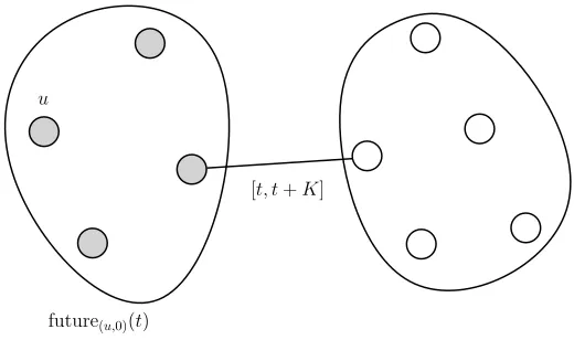
7.2.2. Hearing the Future
In contrast to the previous negative results, we now present an optimal protocol for counting and all-to-all dissemination in dynamic networks with known an upper boundK on theoit, that is based on the following termination criterion. By definition of oit, if future(u,0)(t) = future(u,0)(t+K) then future(u,0)(t) =V. The
reason is that if there exist uninfluenced nodes, then at least one such node must be influenced in at most
K rounds, otherwise no such node exists and (u,0) must have already influenced all nodes (see also Figure 4). So, a fundamental goal is to allow a node to know its future set. Note that this criterion has a very basic difference from all termination criteria that have so far been applied to worst-case dynamic networks: instead of keeping track of its past set(s) and waiting for new incoming influences a node now directly keeps track of its future set and is informed by other nodes of its progress. We assume, for simplicity, a unique leader`in the initial configuration of the system (this is not a necessary assumption and we will soon show how it can be dropped).
ProtocolHear from known. We denote byrthe current round. Each nodeukeeps a listInf luin which it keeps track of all nodes that first heard of (`,0) (the initial state of the leader) byu(uwas between those nodes that first delivered (`,0) to nodes inInf lu), a setAu in which it keeps track of theInf lv sets that it is aware of initially set to (u, Inf lu,1), and a variabletimestampinitially set to 1. Each nodeubroadcast in every round (u, Au) and if it has heard of (`,0) also broadcasts (`,0). Upon reception of an id wthat is not accompanied with (`,0), a nodeuthat has already heard of (`,0) adds (w, r) toInf lu to recall that at roundrit notifiedwof (`,0) (note that it is possible that other nodes also notifywof (`,0) at the same time withoutubeing aware of them; all these nodes will write (w, r) in their lists). If it ever holds at a nodeuthat
r >max(v6=u,r0)∈Inf l
u{r
0
}+Kthen uadds (u, r) inInf lu (replacing any existing (u, t)∈Inf lu) to denote the fact thatris the maximum known time until whichuhas performed no further propagations of (`,0). If at some roundr a nodeumodifies itsInf lu set, it setstimestamp←r. In every round, a nodeuupdates
Auby storing in it the most recent (v, Inf lv, timestamp) triple of each nodevthat it has heard of so far (its own (u, Inf lu, timestamp) inclusive), where the “most recent” triple of a nodev is the one with the greatest
timestampbetween those whose first component is v. Moreover,uclears multiple (w, r) records from the
u
[t, t+K]
[image:15.612.174.434.70.224.2]future(u,0)(t)
Figure 4: If there are still nodes that have not heard fromu, then ifK is an upper bound on theoit, in at mostK rounds another node will hear fromu(by definition of theoit).
those that share (w, r). Similarly, the leader collects all (v, Inf lv, timestamp) triples in its ownA` set. Let
tmaxdenote the maximum timestamp appearing inAl, that is the maximum time for which the leader knows that some node was influenced by (`,0) at that time. Moreover denote byI the set of nodes that the leader knows to have been influenced by (`,0). Note thatI can be extracted fromA` byI ={v ∈ V : ∃u∈ V, ∃timestamp, r ∈ N s.t. (u, Inf lu, timestamp) ∈ A` and (v, r) ∈ Inf lu}. If at some round r it holds at the leader that for all u ∈ I there is a (u, Inf lu, timestamp) ∈ A` s.t. timestamp ≥ tmax+K and max(w6=u,r0)∈Inf l
u{r
0
} ≤tmaxthen the leader outputs|I| orI depending on whether counting or all-to-all dissemination needs to be solved and halts (it can also easily notify the other nodes to do the same inK· |I|
rounds by a simple flooding mechanism and then halt).
The above protocol can be easily made to work without the assumption of a unique leader. The idea is to have all nodes begin as leaders and make all nodes prefer the leader with the smallest id that they have heard of so far. In particular, we can have each node keep an Inf l(u,v) only for the smallest v that it has
heard of so far. Clearly, inO(D) rounds all nodes will have converged to the node with the smallest id in the network.
Theorem 8. Protocol Hear from knownsolves counting and all-to-all dissemination in O(D+K) rounds by using messages of sizeO(n(logK+ logn)), in any dynamic network with dynamic diameterD, and with oit upper bounded by someK known to the nodes.
Proof. In time equal to the dynamic diameterD, all nodes must have heard of `. Then in another D+K
rounds all nodes must have reported to the leader all the direct outgoing influences that they performed up to timeD (nodes that first heard of` by that time) together with the fact that they managed to perform no new influences in the interval [D, D+K]. Thus by time 2D+K = O(D+K), the leader knows all influences that were ever performed, so no node is missing from itsIset, and also knows that all these nodes forK consecutive rounds performed no further influence, thus outputs|I|=n(for counting) orI=V (for all-to-all dissemination) and halts.
Can these termination conditions be satisfied while |I| < n, which would result in a wrong decision? Thus, for the sake of contradiction, assume that tmax is the time of the latest influence that the leader is aware of, that |I| < n, and that all termination conditions are satisfied. The argument is that if the termination conditions are satisfied then (i) I= future(`,0)(tmax), that is the leader knows precisely those
nodes that have been influenced by its initial state up to timetmax. Clearly,I⊆future(`,0)(tmax) as every
node inI has been influenced at most by timetmax. We now show that additionally future(`,0)(tmax)⊆I.
If future(`,0)(tmax)\I 6=∅, then there must exist some u∈I that has influenced a v∈future(`,0)(tmax)\I
at most by time tmax (this follows by observing that ` ∈ I and that all influence paths originate from
`). But now observe that when the termination conditions are satisfied, for each u∈I the leader knows a
it should be aware of the fact that v∈ future(`,0)(tmax), i.e. it should hold that v ∈I, which contradicts
the fact thatv∈future(`,0)(tmax)\I. (ii) The leader knows that in the interval [tmax, tmax+K] no node
inI= future(`,0)(tmax) performed a new influence. These result in a contradiction as|future(`,0)(tmax)|=
|I|< nand a new influence should have occurred in the interval [tmax, tmax+K] (by the fact that theoit
is upper bounded byK).
Optimality follows from the fact that a node u can know at time t that past(u,t)(0) = V only if
past(u,t)(K) = V. This means that u must have also heard of the K-states of all nodes, which requires
Θ(K +D) rounds in the worst case. If past(u,t)(K) 6= V, then it can be the case that there is some v ∈V\past(u,t)(K) s.t. uhas heardv’s 0-state but not its K-state. Such a node could be a neighbor ofu
at round 1 that then moved far away. Again, similarly to Theorem 3, we can have arbitrarily many nodes to have no neighbor until timeK (e.g. in the extreme case wereoit is equal to K) and then from timeK
onwards are only connected to nodev. As uhas not heard from theK-state ofv it also cannot have heard of the 0-state of arbitrarily many nodes.
An interesting improvement is to limit the size of the messages toO(logn) bits probably by paying some increase in time to termination. We almost achieve this by showing that an improvement of the size of the messages toO(logD+ logn) bits is possible (note thatO(logD) =O(logKn)) if we have the leader initiate individual conversations with the nodes that it already knows to have been influenced by its initial state. We have already successfully applied a similar technique in [MCS12a], however in a different context. The protocol, that we callTalk to known, solves counting and all-to-all dissemination inO(Dn2+K) rounds by
using messages of size O(logD+ logn), in any dynamic network with dynamic diameter D, and with oit
upper bounded by someK known to the nodes.
We now describe theTalk to knownprotocol by assuming again for simplicity a unique leader (this, again, is not a necessary assumption).
Protocol Talk to known. As in Hear from known, nodes that have been influenced by the initial state of the leader (i.e. (`,0)) constantly forward it and whenever a node v manages to deliver it then it stores the id of the recipient node in its localInf lv set. Nodes send in each round the time of the latest influence (i.e. the latest new influence of a node by (`,0)), call ittmax, that they know to have been performed so far. Whenever the leader hears of a greatertmaxthan the one stored in its local memory it reinitializes the process of collecting its future set. By this we mean that it waitsKrounds and then starts again from the beginning, talking to the nodes that it has influenced itself, then to the nodes that were influenced by these nodes, and so on. The goal is for the leader to collect precisely the same information as inHear from known. In particular, it sorts the nodes that it has influenced itself in ascending order of id and starts with the smallest one, call it
v, by initiating atalk(`, v, current round) message. All nodes forward the most recent talkmessage (w.r.t. to their timestamp component) that they know so far. Upon receipt of a newtalk(`, v, timestamp) message (the fact that it is “new” is recognized by the timestamp), v starts sending Inf lv to the leader in packets of size O(logn), for example a single entry each time, via talk(v, `, current round, data packet) messages. When the leader receives atalk(v, `, timestamp, data packet) message where data packet=EN D CON V
(for “END of CONVersation”) it knows that it has successfully received the wholeInf lvset and repeats the same process for the next node that it knows to have been already influenced by (`,0) (now also including those that it learned fromv). The termination criterion is the same as inHear from known.
Theorem 9. Protocol Talk to known solves counting and all-to-all dissemination in O(Dn2+K) rounds
by using messages of sizeO(logD+ logn), in any dynamic network with dynamic diameterD, and withoit upper bounded by some K known to the nodes.
Proof. Correctness follows from the correctness of the termination criterion proved in Theorem 8. For the bit complexity we notice that the timestamps and tmaxare of size O(logD) (which may beO(logKn) in the worst case). The data packet and the id-components are all of size O(logn). For the time complexity, clearly, inO(D) rounds the final outgoing influence of (`,0) will have occurred and thus the maximumtmax
talk ton−1 nodes each believing that it performedn−1 deliveries (this is because in the worst case it can hold that any new node is concurrently influenced by all nodes that were already influenced and in the end all nodes claim that they have influenced all other nodes) thus, in total, it has to wait forO(n2) data packets
each takingO(D) rounds to arrive. TheK in the bound is from the fact that the leader waitsK rounds after reinitializing in order to allow nodes to also report whether they performed any new assignments in the [tmax, tmax+K] interval.
8. Conclusions
To the best of our knowledge, this is the first study of worst-case dynamic networks that are free of any connectivity assumption about their instances. To enable a quantitative study we proposed some novel generic metrics that capture the speed of information propagation in a dynamic network. We proved that fast dissemination and computation are possible even under continuous disconnectivity. In particular, we presented optimal termination conditions and protocols based on them for the fundamental counting and all-to-all token dissemination problems.
There are many open problems and promising research directions related to this work. We would like to improve the existing lower and upper bounds for counting and information dissemination. The best lower bound known for k-token dissemination is Ω(nk/logn) (even for centralized algorithms on networks with connected instances and messages of size O(logn)) [DPR+13] while our upper bound isO(Dn2+K)
(for messages of size O(logD+ logn)). Techniques from [HCAM12] or related ones may be applicable to achieve quick token dissemination. It would be also important to refine the metrics proposed in this work so that they become more informative. For example, the oit metric, in its present form, just counts the time needed for another outgoing influence to occur. It would be useful to define a metric that counts the number of new nodes that become influenced per round which would be more informative w.r.t. the speed of information spreading. An interesting variation of our metrics, which is due to a reviewer of this article, is to define them in an amortized way. For example, oit =k can alternatively be defined as
h=|future(u,t)(t0)| ≥min{h+b(t0−t)/kc, n} and this weaker definition may be of high practical value as,
this way, the class of dynamic graphs havingoit=k(which now can also be fractional) will be much larger. An asynchronous communication model in which nodes can broadcast when there are new neighbors would be a very natural extension of the synchronous model that we studied in this work. Note that in our work (and all previous work on the subject) information dissemination is only guaranteed under continuous broad-casting. How can the number of redundant transmissions be reduced in order to improve communication efficiency? Is there a way to exploit visibility to this end? Does predictability help (i.e. some knowledge of the future)? Finally, randomization will be certainly valuable in constructing fast and symmetry-free protocols. We strongly believe that these and other known open questions and research directions will motivate the further growth of this emerging field.
Acknowledgements
We would like to thank some anonymous reviewers for carefully reading the manuscript and for providing valuable comments that have helped us to improve our work substantially.
References
[AAD+06] D. Angluin, J. Aspnes, Z. Diamadi, M. J. Fischer, and R. Peralta. Computation in networks of
passively mobile finite-state sensors. Distributed Computing, pages 235–253, March 2006.
[AKL08] C. Avin, M. Kouck´y, and Z. Lotker. How to explore a fast-changing world (cover time of a simple random walk on evolving graphs). InProceedings of the 35th international colloquium on Automata, Languages and Programming (ICALP), Part I, pages 121–132, Berlin, Heidelberg, 2008. Springer-Verlag.
[APRU12] J. Augustine, G. Pandurangan, P. Robinson, and E. Upfal. Towards robust and efficient computa-tion in dynamic peer-to-peer networks. InProceedings of the Twenty-Third Annual ACM-SIAM Symposium on Discrete Algorithms (SODA), pages 551–569. SIAM, 2012.
[AW04] H. Attiya and J. Welch. Distributed computing: fundamentals, simulations, and advanced topics, volume 19. Wiley-Interscience, 2004.
[BCF09] H. Baumann, P. Crescenzi, and P. Fraigniaud. Parsimonious flooding in dynamic graphs. In Proceedings of the 28th ACM symposium on Principles of distributed computing (PODC), pages 260–269. ACM, 2009.
[Bol98] B. Bollob´as. Modern Graph Theory. Springer, corrected edition, July 1998.
[CFQS12] A. Casteigts, P. Flocchini, W. Quattrociocchi, and N. Santoro. Time-varying graphs and dynamic networks. International Journal of Parallel, Emergent and Distributed Systems, 27[5]:387–408, 2012.
[CMM+08] A. E. Clementi, C. Macci, A. Monti, F. Pasquale, and R. Silvestri. Flooding time in
edge-markovian dynamic graphs. InProceedings of the twenty-seventh ACM symposium on Principles of distributed computing (PODC), pages 213–222, New York, NY, USA, 2008. ACM.
[CMN+11] I. Chatzigiannakis, O. Michail, S. Nikolaou, A. Pavlogiannis, and P. G. Spirakis. Passively
mobile communicating machines that use restricted space. Theor. Comput. Sci., 412[46]:6469– 6483, October 2011.
[Dol00] S. Dolev. Self-stabilization. MIT Press, Cambridge, MA, USA, 2000.
[DPR+13] C. Dutta, G. Pandurangan, R. Rajaraman, Z. Sun, and E. Viola. On the complexity of
informa-tion spreading in dynamic networks. InProc. of the 24th Annual ACM-SIAM Symp. on Discrete Algorithms (SODA), 2013.
[Hae11] B. Haeupler. Analyzing network coding gossip made easy. In Proceedings of the 43rd annual ACM symposium on Theory of computing (STOC), pages 293–302. ACM, 2011.
[HCAM12] B. Haeupler, A. Cohen, C. Avin, and M. M´edard. Network coded gossip with correlated data. CoRR, abs/1202.1801, 2012.
[KKK00] D. Kempe, J. Kleinberg, and A. Kumar. Connectivity and inference problems for temporal networks. InProceedings of the thirty-second annual ACM symposium on Theory of computing (STOC), pages 504–513, 2000.
[KLO10] F. Kuhn, N. Lynch, and R. Oshman. Distributed computation in dynamic networks. In Proceed-ings of the 42nd ACM symposium on Theory of computing (STOC), pages 513–522, New York, NY, USA, 2010. ACM.
[KMO11] F. Kuhn, Y. Moses, and R. Oshman. Coordinated consensus in dynamic networks. InProceedings of the 30th annual ACM SIGACT-SIGOPS symposium on Principles of distributed computing (PODC), pages 1–10, 2011.
[Lam78] L. Lamport. Time, clocks, and the ordering of events in a distributed system. Commun. ACM, 21[7]:558–565, 1978.
[Lyn96] N. A. Lynch. Distributed Algorithms. Morgan Kaufmann; 1st edition, 1996.
[MCS11a] O. Michail, I. Chatzigiannakis, and P. G. Spirakis. Mediated population protocols. Theor. Comput. Sci., 412[22]:2434–2450, May 2011.
[MCS11b] O. Michail, I. Chatzigiannakis, and P. G. Spirakis. New Models for Population Protocols. N. A. Lynch (Ed), Synthesis Lectures on Distributed Computing Theory. Morgan & Claypool, 2011.
[MCS12a] O. Michail, I. Chatzigiannakis, and P. G. Spirakis. Brief announcement: Naming and counting in anonymous unknown dynamic networks. InProceedings of the 26th international conference on Distributed Computing (DISC), pages 437–438, Berlin, Heidelberg, 2012. Springer-Verlag.
[MCS12b] O. Michail, I. Chatzigiannakis, and P. G. Spirakis. Causality, influence, and computation in possi-bly disconnected synchronous dynamic networks. In16th International Conference on Principles of Distributed Systems (OPODIS), pages 269–283, 2012.
[MMCS13] G. B. Mertzios, O. Michail, I. Chatzigiannakis, and P. G. Spirakis. Temporal network opti-mization subject to connectivity constraints. In 40th International Colloquium on Automata, Languages and Programming (ICALP), volume 7966 of Lecture Notes in Computer Science, pages 663–674. Springer, July 2013.
[OW05] R. O’Dell and R. Wattenhofer. Information dissemination in highly dynamic graphs. In Proceed-ings of the 2005 joint workshop on Foundations of mobile computing (DIALM-POMC), pages 104–110, 2005.
[Sch02] C. Scheideler. Models and techniques for communication in dynamic networks. InProceedings of the 19th Annual Symposium on Theoretical Aspects of Computer Science (STACS), pages 27–49, 2002.