Searching Large Scale Image Collections

(1)

Searching Large-Scale Image Collections

Thesis by

Mohamed Alaa El-Dien Mahmoud Hussein Aly

In Partial Fulfillment of the Requirements

for the Degree of

Doctor of Philosophy

California Institute of Technology

Pasadena, California

2011

(2)

Mohamed Alaa El-Dien Mahmoud Hussein Aly

(3)

iii

To my family: my mother, my father, my wife and kids, and my sister. They have always

(4)

Acknowledgments

First and foremost, all thanks are due to God, for giving me the strength and persistence to

go through six years of graduate work.

Second, I would like to thank my thesis adviser, Prof. Pietro Perona, for being an

ex-ceptional adviser, both academically and professionally. I learned a lot from his knowledge,

insight, and guidance.

Third, I would like to thank Prof. Yaser Abu-Mostafa. He was my initial co-adviser at

Caltech. He gave me invaluable advice and patiently and graciously helped me refine and

define my thesis topic.

Fourth, I would like to thank Dr. Mario Munich for hosting me for an internship at

Evolution Robotics, and for collaborating with me and providing me with advice during all

my thesis work.

Fifth, I would like to thank Dr. Jean-Yves Bouguet for hosting me for one internship at

Google, and helping me get a second one. I would also like to thank Dr. Drago Anguelov,

Dr. James Philbin, Dr. Hartwig Adam, and Dr. Hartmut Neven for their great help in

the second internship at Google, in which I was able to perform the large-scale distributed

experiments of Chapter 7.

(5)

Vi-v

sion Lab, who helped make my time possible. Specifically, I would like to thank Peter

Welinder for helping me collect some of the datasets, and co-authoring a couple of papers.

I would also like to thank Marco Andreetto and Ahmed Elbanna for helpful and insightful

discussions.

Finally, I would like to thank my family. My parents have always supported and pushed

me, starting from elementary school and up to graduate school. My wife and kids also

supported me and have been very patient with me taking time away from them in order to

(6)

Abstract

Searching quickly and accurately in a large collection of images has become an increasingly

important problem. The ultimate goal is to make visual search possible: allow users to

search using images in addition to typing text. The typical approach is to index all the

images of interest (e.g., images of landmarks, books, or DVDs) in a database and let users

question the system with query images. Such a database can reach billions of images, and

this poses challenges in terms of memory and computational requirements and recognition

performance. In this work we provide an in depth study of systems used for searching

large-scale image collections.

Specifically, we provide a thorough comparison of the two leading image search

ap-proaches: Full Representation (FR) vs. Bag of Words (BoW). We derive theoretical

es-timates of how the memory and computational cost scale with the number of images in

the database, and empirically evaluate the performance and run time on four real-world

datasets. Our experiments suggest that FR provides better recognition performance than

BoW, though it requires more memory. Therefore, we address these shortcomings by

pre-senting novel methods that increase the recognition performance of BoW and decrease the

memory requirements of FR. Finally, we present a novel way to parallelize FR on multiple

(7)

vii

List of Figures

2.1 Basic Image Search Problem . . . 7

2.2 Object Category Recognition Vs. Specific Object Recognition . . . 8

2.3 Object Recognition Flavors . . . 9

2.4 Image Representations . . . 9

2.6 Full Representation (FR) Image Search . . . 13

2.7 Bag of Words (BoW) Image Search . . . 14

2.8 Kd-Trees (Kdt) . . . 15

2.9 Locality Sensitive Hashing (LSH) . . . 18

2.10 Hierarchical K-Means (HKM) . . . 19

2.11 BoW Inverted File (IF) Search . . . 21

2.12 BoW Min-Hash (MH) Search . . . 23

3.1 Theoretical Scaling Properties . . . 30

3.2 Kd-Tree Parallelizations . . . 31

3.3 Parallelization Run Time . . . 31

4.1 Probe and Distractor Sets . . . 53

(13)

xiii

4.3 Example Distractor Images . . . 56

4.4 Recognition Performance and Time Vs. Dataset Size . . . 60

4.5 Recognition Performance Vs. Time . . . 61

4.6 Run Time: Theory Vs. Practice . . . 63

4.7 Recognition Performance and Time Vs. Dataset Size (Full) . . . 64

4.8 Recognition Performance Vs. Time (Full) . . . 65

4.9 Kd-Tree Parameter Tuning . . . 67

4.10 LSH-L2 Parameter Tuning . . . 69

4.11 LSH-Sim Parameter Tuning . . . 70

4.12 LSH-Orth Parameter Tuning . . . 71

4.13 Hierarchical K-Means Parameter Tuning . . . 73

4.14 Quick Tuning for Inverted File . . . 75

4.15 Full Tuning for Inverted File . . . 76

4.16 Quick Tuning for Min-Hash. . . 77

4.17 Full Tuning for Min-Hash . . . 78

5.1 Ordinary Vs. Compact Kd-Tree . . . 86

5.2 Recognition Performance for Binary Signatures and PCA . . . 88

5.3 Recognition Performance for Compact Kd-Tree . . . 90

5.4 Comparison of CompactKdt with BoW . . . 93

6.1 Multiple Dictionaries for BoW . . . 96

6.2 MDBoW Memory and Computational Requirements . . . 99

(14)

6.4 Parallelization of Multiple Dictionaries for BoW . . . 102

6.5 Model Features Results . . . 104

6.6 Combining Multiple Dictionaries with Model Features . . . 105

6.7 MDBoW Precision@kResults . . . 106

7.1 Canonical MapReduce Example . . . 109

7.2 Kd-Tree Parallelizations . . . 111

7.3 Parallel Kd-Tree MapReduce Schematic . . . 113

7.4 Effect of Distance ThresholdSt . . . 116

7.5 Effect of Backtracking StepsB . . . 117

7.6 Effect of Number of MachinesM . . . 117

7.7 Effect of the Number of Images . . . 119

7.8 Precision@1 Vs. Throughput . . . 119

7.9 Throughput: Theory Vs. Practice . . . 120

7.10 Throughput Vs. the Number of Root Machines . . . 121

7.11 Precision@kfor DKdt . . . 122

(15)

xv

List of Tables

2.1 Search Methods Abbreviations . . . 24

3.1 Methods Parameter Definitions and Typical Values . . . 28

3.2 Theoretical Scaling Properties . . . 29

4.1 Probe Sets . . . 55

4.2 Evaluation Scenarios . . . 58

4.3 Experimental Comparison Parameter Settings . . . 59

5.1 Kd-Tree Parameter Definitions . . . 81

5.2 Storage Savings for Using Binary Signatures with Kd-Trees . . . 84

5.3 BoW Parameter Definitions . . . 91

5.4 CompactKdt and BoW Storage and Computational Cost Comparison . . . . 91

(16)

List of Algorithms

2.2 Randomized Kd-Trees Construction . . . 16

2.3 Randomized Kd-Trees Search . . . 16

5.1 Compact Kd-Trees (CompactKdt) . . . 85

6.1 Multiple Dictionaries for Bag of Words (MDBoW) . . . 97

(17)

1

Chapter 1 Introduction

Searching for a specific object in a large-scale collection of images has become an

in-creasingly important problem with numerous applications, especially with the popularity

of smart phones. There are currently several applications that allow users to take a photo

with the smart phone camera and search a database of stored images, e.g., Google Goggles

and Barnes and Noble. The ultimate goal of such applications is to make visual search a

reality. In other words, to allow users to search the Internet using images, as it is possible

now to search the Internet using text.

Typical scenarios for visual search include searching images of book covers, DVD

cov-ers, retail products, and buildings and landmarks. The size of databases involved vary from

hundreds of thousands to potentially millions of images, but they could conceivably reach

billions. After building an index using these images, users query the database with a probe

image containing an object of interest, e.g., an image of a book cover from a certain

view-point and scale. The system should respond with the identity of that book together with

some useful information about it, like links to buy it online. All this process should take

only a few seconds, and should work with high precision.

(18)

working image search system that is physically realizable, works with high precision, and

is scalable to hundreds of millions of images, all while working interactively with users.

Obviously building such a system is not an easy task, and poses a lot of challenges, namely

memory requirements, computational cost, and recognition performance. For example, if

we consider 1 billion images, and store on average 100 KB per image, we need to store

100 TB of data just for the feature descriptors, and naively searching for the nearest feature

in a database of 1012 features takes 4 minutes on a supercomputer with 1 TFLOPS. This

is clearly not satisfactory: most applications of interest are interactive and require fast

response time on the order of a few seconds. In turn, this implies the need to store image

descriptors in storage that is very close to the processor, e.g., RAM (with top-of-the-line

machines nowadays having around 50 GB of RAM).

To this end, we start with a comprehensive comparison of the two leading image search

approaches, and study how their properties scale with large number of images both

theoret-ically and experimentally. Both approaches are based on extracting local features from the

images (see Chapter 2 for details), and then indexing these features or some information

extracted therefrom. This information is then used to quickly find the best match of a probe

image in the database images. The first approach, theFull Representation(FR) approach,

stores the features of the database image in exact or compressed form, and efficiently

in-dexes each feature of the probe image into this database. The second approach, the Bag

of Words(BoW), is based on quantizing features into visual words and representing each

image with a histogram of visual words. Our experiments suggest that that FR methods

(19)

3

better memory usage with worse performance (see Chapter 4).

Based on this comparison, we then explore ways to remedy the shortcomings of both

approaches. Specifically, we explore ways to reduce the memory usage of FR methods,

specially with Kd-Trees (Chapter 5). We present Compact Kd-Trees, which are able to

achieve an order of magnitude less memory usage by compressing the local features, while

achieving comparable recognition performance. We also explore ways to boost the

recog-nition performance of BoW methods (Chapter 6). We present Multiple Dictionaries for

BoW, which is able to significantly boost the recognition performance of BoW approach,

albeit with more computational and memory requirements. Finally, we focus on the

par-allelization of FR methods, specially Kd-Trees, so that the system can handle millions of

images (Chapter 7). We present Distributed Kd-Trees, which provide excellent recognition

performance running on a database with 100 million images while processing input images

in a fraction of a second.

This thesis makes a number of contributions:

1. We provide a comprehensive comparison of the two leading image indexing

ap-proaches: Full Representation and Bag of Words. In particular, we provide:

(a) Theoretical estimates of the memory requirements, computational cost, and

par-allelizability of these methods as a function of the number of images.

(b) Experimental evaluation of these different methods on four real world datasets.

We report the recognition performance and run time as the number of images

grows.

(20)

the FR approach is the way to go, since, although it requires an order of magnitude

more storage, it provides superior recognition performance to BoW, especially with

large datasets.

3. We present novel methods to remedy some of the shortcomings of these two methods:

(a) Compact Kd-Trees that are able to cut the memory usage and run time of FR

methods by an order of magnitude while achieving comparable recognition

per-formance.

(b) Multiple Dictionaries for BoW that are able to significantly boost the

recogni-tion performance of BoW methods to levels comparable to FR methods, at the

expense of increased memory and computational costs.

4. We present a novel way of parallelizing Kd-Trees, Distributed Kd-Trees, and run

experiments on thousands of machines with 100 million images. The system

outper-forms the state-of-the-art in both recognition performance and throughput, and can

process a query image in a fraction of a second.

The thesis is organized as follows: in Chapter 2 we give an overview of the approaches

explored in the rest of the thesis and the basic image search algorithm considered. Chapter

3 details the theoretical estimates of the different properties of these approaches and how

they scale up with billions of images. Chapter 4 presents the experimental evaluation of the

different methods on four datasets. Chapter 5 explains a novel method, Compact Kd-Tree,

to reduce the memory usage of the FR approach with comparable recognition performance.

(21)

recogni-5

tion performance of the BoW approach. Chapter 7 gives the implementation details of

Distributed Kd-Trees, and presents experiments on thousands of machines with millions of

(22)

Chapter 2 Methods Overview

2.1 Introduction

In this chapter we give an overview of the image search problem considered in this

the-sis. We then explain the basic image search algorithm, and its relation to the two leading

approaches: Full Representation and Bag of Words. Finally, we finish by describing the

different variants of these two approaches that we consider later in the comparison. Section

2.2 describes the image search problem we consider in this thesis. Section 2.3 describes the

different image representations. Section 2.4 gives an overview of the basic image search

algorithm. Finally, Section 2.5 describes the Full Representation approach, followed by the

Bag of Words approach in Section 2.6.

2.2 Image Search Problem

The basic problem we consider in this thesis is image search. We have a database that

stores images of objects of interest, for example DVD covers, book covers, and landmarks

(23)

7

Figure 2.1: Basic Image Search Problem. The system contains a database that indexes

images of objects of interest. Users can query the system using images taken with their cell phones. The system searches its database and replies with the identity of the query object together with some useful information.

an image of the pyramids, and to query the database using that query image. The system

then searches its database and responds with the identity of the object depicted in the query

image, presenting its stored canonical image and any additional information about that

object.

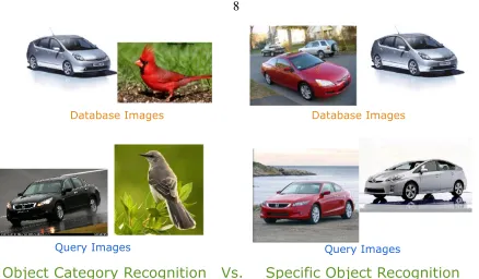
The image search can be done in one of two ways: Object Category Recognition or

Specific Object Recognition (see Figure 2.2). In category recognition, the database images

and the query images do not necessarily represent objects of the same identity, but of the

same category. For example, the query images for object category “sedan car”, can

rep-resent a Honda Accord, while there might not be an image of such object in the database.

The goal of such systems is to identify the category of the object, e.g., a car vs. a bird,

rather than identifying the identity of the object. In specific object recognition, on the other

(24)

[image:24.612.108.546.53.309.2]

Figure 2.2:Object Category Recognition(left)Vs. Specific Object Recognition(right). In this thesis, we focus on specific object recognition.

model of the car. In this thesis we focus only on specific object recognition rather than

category recognition. The systems we are interested in should return the identity of the

specific object depicted in the query image.

Specific object recognition can in turn be divided into three cases (see Figure 2.3): (a)

Scene to Object: where the database image depicts a canonical cropped version of the

object (for example Eiffel Tower), while the query image contains the object of interest in

addition to other objects. (b) Object to Scene: the opposite of case (a), where the database

image contains different objects of interest, while the query image contains only one object.

(c) Object to Object: where both the query and database images contain clean cropped

(25)

9

Figure 2.3: Object Recognition Flavors. (a) Scene to Object: database image depicts

cropped version of objects while query image contains different objects. (b) Object to Scene: opposite of (a). (c) Object to Object: both query and database images contain only one clean cropped version of the object. In this thesis, we focus on (c).

2.3 Image Representation

Figure 2.4: Image Representations. Global features (left) represent an image by one

multi-dimensional feature descriptor, whereas local features (right) represent an image by

a set of features extracted from local regions in the image.

For any image processing operation, we need to represent an image by features extracted

therefrom. The raw image is perfect for the human eye to extract all information from,

(26)

represent images in computer vision (see Figure 2.4):

1. Global features: where the image is represented by one multi-dimensional feature, describing the information in the image. The information can be color histograms

[18], edge magnitude or orientation histograms [15], or a specific descriptor extracted

from some filters applied to the image, such as GIST features [28]. The advantages

of global features are that they are fast and easy to compute and generally require

small amounts of memory. However, they have been shown to perform worse than

the other type, local features [17].

2. Local features: where the image is represented by a set of local feature descriptors extracted from a set of regions around the image. There are generally two

compo-nents for local features: a feature detector and a feature descriptor [18, 25]. A feature

detector detects interesting locations in the image, for example corners and edges.

A feature descriptor describes the image patch around that interest point, usually by

histograms of gradients or orientation. There are different kinds of feature detectors,

but among the most common ones are Difference of Gaussians (DoG) [24],

Hessian-Affine, and Harris Affine [25]. Similarly there are various feature descriptors, but

by far SIFT [24] and HOG [15] are the most widely used. The main advantage of

local features is their superior performance, however they usually have much larger

memory usage, as a typical image can have hundreds of local features [17].

In this thesis we focus on using local features for large-scale image search, since they have

(27)

11

Algorithm 2.1 Basic Image Search Algorithm Image Index Construction

1. Extract local features{fi j}j from every database imagei.

2. Store some function of these featuresg(fi j)and build data structure d(g) based on

g(). In the data structure each featureg(fi j)is associated to one (or more) database

images that contain that feature.

Image Index Search

1. Given the probe image, extract its local featuresfq j and computeg(fq j).

2. Search through the data structured(g)for “nearest neighbors”.

3. Every nearest neighbor votes for one (or more) database image(s)ithat it is

associ-ated to.

4. Sort the database images based on their scoresi.

5. Post-process the sorted list of images to enforce some geometric consistency and

obtain a final list of sorted imagess′_i. The geometric consistency check is done using

a RANSAC algorithm to fit an affine transformation between the positions of the

matched features in the query imageqand the database imagei.

2.4 Basic Image Search Algorithm

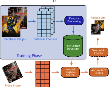
The basic local features image search algorithm is depicted in Figure 2.5 and detailed in

Algorithm 2.1. The two main steps are:

1. Training phase: where the image index is constructed. Local features are extracted from the input images, and are inserted (optionally after some post-processing) into a

data structure that allows for fast approximate nearest-neighbor search. Several types

of these data structures, or indices, will be discussed in Sections 2.5 and 2.6.

2. Query phase: where the image index is searched for a query image. Every local fea-ture in the query image is used to search the database feafea-tures for nearest neighbors.

(28)

[image:28.612.151.498.56.334.2]

Figure 2.5: Basic Image Search Algorithm. In the training phase, local features are extracted from the database images, optionally processed, and then inserted into a fast search data structure. At query time, local features are extracted from the query image, and for each such feature the index is searched for nearest neighbors. Scores are accumulated for each database image, and a final ranked list of result images is presented to the user. See Algorithm 2.1.

system can then perform post-processing to verify the geometric consistency of the

feature locations in the image. The final result is a ranked list of database images,

with high ranked images being more likely to correspond to the query image.

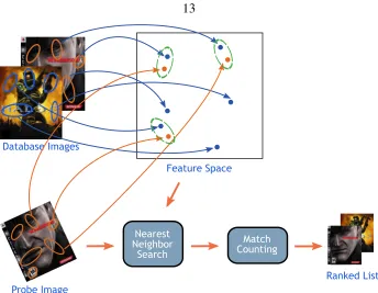
There are two leading approaches for building such large-scale image indexing systems:

1. Full Representation (FR): where the feature space is searched directly for nearest neighbors using the full features [24, 4, 3] (see Figure 2.6).

(29)

[image:29.612.152.496.51.318.2]

13

Figure 2.6: Full Representation Image Search. The nearest-neighbor search is done

directly in the feature space, as opposed to BoW search which uses quantization in the feature space (see Figure 2.7).

2.7).

Each of these two approaches have a number of variants that use different techniques to

perform the actual search. These techniques have a lot of parameters that affect their

recognition performance, run time, and memory requirements. In the following we will

briefly describe these techniques and list their parameters, and we will explore their effect

experimentally in Chapter 4.

2.5 Full Representation (FR) Image Search

In FR image search (see Figure 2.6), the feature space is searched directly for nearest

(30)

[image:30.612.151.499.53.299.2]

Figure 2.7: Bag of Words Image Search. The nearest-neighbor search is done indirectly via vector quantization of the feature space, as opposed to directly searching the feature space as in FR search (see Figure 2.6).

The specifics from Algorithm 2.1 are:

1. The functiong(fi j) =fi j is the identity function, i.e., the full features are stored

2. The data structured({fi j}i j)is designed for efficient nearest neighbor lookup at the

expense of some additional storage.

We consider three general methods for performing nearest neighbor search in the feature

space: Kd-Trees, Locality Sensitive Hashing, and Hierarchical K-Means.

2.5.1 Kd-Trees (Kdt)

One (or more) randomized Kd-trees [6, 24] are built for the database features {fi j}i j to

(31)

15

Figure 2.8: Kd-Trees (Kdt). (Left) A Kd-Tree in two dimensions. (Right) A set of

ran-domized Kd-Trees. See Section 2.5.1.

Algorithm 2.2 explains the Kd-Tree construction procedure, while Algorithm 2.3 details

the search procedure.

Kd-Trees have two parameters that affect their recognition performance, storage, and

run time:

1. T: the number of trees, where having more trees increases accuracy without much

affecting speed, due to the single search queue. However, this increases the storage

required due to the need to store the additional trees.

2. B: the number of backtracking steps, which poses a trade off between accuracy and

speed. Having more steps will give more accuracy but takes more time.

2.5.2 Locality Sensitive Hashing (LSH)

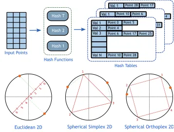
A number of locality sensitive hash functions [5, 23] are extracted from the database

(32)

Algorithm 2.2 Randomized Kd-Trees Construction Input: A set of vectors{xi} ∈RN

Output: A set of binary Kd-Trees {Tt}. Each internal node has a split (dim,val) pair

where dim is the dimension to split on and val is the threshold such that all points with

xi[dim]≤val belong to the left child and the rest belong to the right child. The leaf nodes

have a list of indices to the features that ended up in that node.

Operation: For each treeTt:

1. Assign all the points{xi}to the root node.

2. For verynodein the tree visited in breadth-first order, compute the split as follows:

(a) For each dimensiond=1. . .N, compute its meanmean(d)and variancevar(d)

from the points in that node.

(b) Choose a dimensiondr at random from the variances within 80% of the

maxi-mum variance.

(c) Choose the split value as the mean of that dimensionmean(dr).

(d) For all points that belong to this node: if x[dr] ≤ mean(dr) assign x to

le f t[node], otherwise assignxtoright[node].

Algorithm 2.3 Randomized Kd-Trees Search

Input: A set of Kd-Trees{Tt}, a set of vectors {xi} ∈RN used to build the trees, a query

vectorq∈RN, maximum number of backtracking stepsB

Output: A set ofknearest neighbors{n_k}with their distances{d_k}to the query vectorq.

Operation:

1. Initialize a priority queueQ with the root nodes of thet trees by adding branch=

(t,node,val)with val=0. The queue is indexed by val[branch], i.e., it returns the

branch with smallestval.

2. count = 0. list= [].

3. Whilecount ≤B:

(a) Retrieve the topbranchfromQ.

(b) Descend the tree defined by branch till lea f, adding unexplored branches on

the way toQ.

(c) Add the points inlea f tolist.

4. Find the k nearest neighbors to q in list and return the sorted list {n_k} and their

(33)

17

hash functions, which are then concatenated to get the index of the bucket within the table

where the feature should go. All features with the same hash value go to the same bucket.

At query time, the hash value is computed for the query feature. Only features in buckets

with this value need to be further processed for nearest neighbors. Three different hash

functions are considered:

1. L2: this approximates the Euclidean distance [5], where the hash function ish(x) =

j_<

x,r>+b

w

k

where< ., . >is the dot product,ris a random unit vector,bis a random

offset, andwis the bin width. For normalized feature vectors, it basically projects the

feature onto a random direction and then returns the bin number where the projection

lies.

2. Spherical-Simplex: this approximates distances on the hypersphere [33], where the

hash function ish(x) =argmin_ihx,yii, whereyiare the vertices of a random simplex

inscribed in the unit hypersphere. The hash value is the index of the nearest vertex of

the simplex.

3. Spherical-Orthoplex: this approximates distances on the hypersphere [33], where

the hash function is h(x) = argmin_ihx,yii, where yi are the vertices of a random

orthoplex inscribed in the unit hypersphere. The hash value is the index of the nearest

vertex of the orthoplex.

There are generally two parameters for any LSH method:

1. T: the number of tables. Generally, having more tables improves performance but

(34)

2. H: the number of hash functions. Having more functions increases run time, but

makes collisions, and hence bucket size, less.

In addition, L2 LSH includes one more parameter, which isw, the bin size for the

[image:34.612.141.498.193.465.2]

projec-tion.

Figure 2.9:Locality Sensitive Hashing (LSH). (Top) A schematic of LSH search. A set of

hash functions are extracted for each feature, and features with the same hash values go to the same bucket in each hash table. At query time, only buckets with the same hash value

as the query feature need to be searched. (Bottom) Three different hash functions in two

dimensions: L2, Spherical Simplex, and Spherical Orthoplex. See Section 2.5.2.

2.5.3 Hierarchical K-Means (HKM)

A hierarchical decomposition [27] is built from the database features{fi j}i j. At each level

of the tree, the features that are associated with the current node are clustered using

(35)

19

Figure 2.10: Hierarchical K-Means (HKM). (Left) HKM in two dimensions. (Right) A

schematic of the HKM search tree. See Section 2.5.3.

(see Figure 2.10). At query time, the tree is traversed using the query feature, until it

reaches a leaf, in which case those features in the leaf are processed for the nearest neighbor.

Backtracking can also be performed on the tree [26], but is not considered in this work.

There are two parameters that affect the amount of storage and running time of HKM:

1. D: the maximum depth of the tree. A deeper tree requires more storage, but reduces

the run time (for a fixed number of features), as the number of features in the leaves

will be smaller.

2. k: the branching factor of the tree. A largerk also requires more storage, since we

will need to store more cluster centers in the internal nodes. However, for a fixed

number of features, it reduces the run time since it creates more leaf nodes in the

(36)

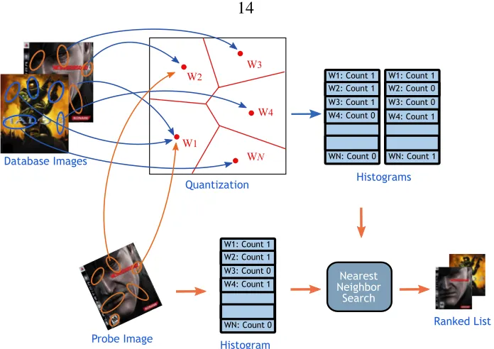
2.6 Bag of Words (BoW) Image Search

In BoW image search (see Figure 2.7), the nearest-neighbor search is done using

quan-tization in the feature space. Two features are considered matched if they belong to the

same cluster, or “visual word”, in the feature space [32, 12, 30, 3]. This is inspired by the

text search literature where documents are represented by the frequency of the words they

contain [36]. The specifics from Algorithm 2.1 are:

1. The functiong(fi j)represents a vector quantization of the input features. The

“dictio-nary” used for quantization is built from the database images by clustering features

into representative “visual words”. Then, each image is represented by a histogram

of occurrences of these visual words{hi}i, and the original local feature vectors are

thrown away.

2. The data structure d({fi j}i j) is designed for efficient nearest-neighbor lookup for

histograms of visual words{hi}i.

In the training phase, the image features are “quantized”, i.e., each feature is assigned to the

closed visual word. Then, the images are represented by histograms of these visual words,

which are then stored in a data structure that allows fast histogram search (see Sections

2.6.1 and 2.6.2). At query time, the histogram of the query image is computed, and used

to query the data structure for the image with the closest histogram. We consider two data

structures that try to perform faster search through the database histograms: Inverted File

(37)

[image:37.612.110.539.55.316.2]

21

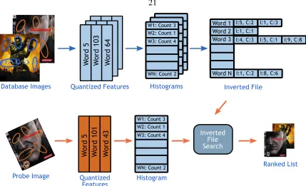
Figure 2.11: BoW Inverted File (IF) Search. The image features are extracted, quantized,

and then converted into histograms of visual words. The histograms are stored in an in-verted file, which is then searched with the histogram of the query image for the nearest neighbor. See Section 2.6.1.

2.6.1 Inverted File (IF)

The idea is to store for every visual word the list of images that contain it (see Figure 2.11).

At run time, only images with overlapping words are processed, and this saves a lot of time

and provides exact search results [7, 36].

Inverted files have several parameters that affect performance and storage requirements,

including the number of visual words, histogram weighting, normalizations, dictionary

generation method, and distance functions:

• W: the number of visual words. Typically, this is in the order of hundreds of

thou-sands to a million [30, 20, 2]. Using fewer visual words usually results in worse

(38)

perfor-mance, except when done in a special way (see Chapter 6). Also using more visual

words increases the search speed due to the lower probability of overlap between

image histograms.

• Weighting: whether to use the raw histogram, or modify the histogram counts

1. none: use the raw histogram

2. binary: binarize the histogram, i.e., just record whether the image has the visual word or not

3. tf-idf: weight the counts in such a way to decrease the influence of more com-mon words and increase the influence of more distinctive words

• Normalizations: how to normalize the histograms

1. l1: normalize so that they sum to one, i.e.,∑i|hi|=1

2. l2: normalize so they have unit length, i.e.,∑ih2i =1

• Distance: what distance function to use between histograms

1. l1: use the sum of absolute differences, i.e.,dl1(h,g) =∑i|hi−gi|

2. l2: use the sum of squared differences, i.e.,dl2(h,g) =∑i(hi−gi)

2

3. cos: use the dot product, i.e., dcos(h,g) = 2−∑ihi×gi. (Note that for l2

-normalized histograms, this is equivalent tol2distance since||h||2=||g||2=1

anddl2=||h−g||22=||h||22+||g||22−2∑ihigi=2−2∑ihigi, i.e., they give the

(39)

[image:39.612.108.540.54.319.2]

23

Figure 2.12: BoW Min-Hash (MH) Search. The image features are extracted, quantized,

and then converted into histograms of visual words. The histograms are binarized, and used to build a set of Min-Hash tables. The histogram of the query image is then used to search for the nearest neighbor in Min-Hash tables. See Section 2.6.2.

• Dictionary Generation: what method to use for generating the visual words (feature space quantization)

1. Approximate K-Means (AKM): which approximates the nearest-neighbor search within K-Means using a set of randomized Kd-Trees [30].

2. Hierarchical K-Means (HKM): which builds a vocabulary tree by applying K-Means recursively [27] at each node in the tree.

2.6.2 Min-Hash (MH)

A number of locality sensitive hash functions [9, 10, 8, 12] are extracted from the database

(40)

binarized (counts are ignored), and each image is represented as a “set” of visual words

{bi}i. The hash function is defined ash(b) =minπ(b)whereπ is a random permutation

of the numbers{1, ...,W}, whereW is the number of words in the dictionary.

There are three parameters that affect the performance of MH image search:

1. W: the number of visual words in the dictionary. Generally, the larger the dictionary,

the better the performance and the faster the actual search, because the number of

overlapping images is smaller.

2. T: the number of hash tables.

3. H: the number of hash functions.

2.7 Summary

Full name Abbreviation Section

Full Representation FR 2.5

Exhaustive exhaustive 2.5

Kd-Trees Kdt 2.5.1

Locality Sensitive Hashing LSH 2.5.2

LSH with L2 LSH-L2 2.5.2

Spherical LSH with Simplex LSH-Sim 2.5.2

Spherical LSH with Orthoplex LSH-Orth 2.5.2

Hierarchical K-Means HKM 2.5.3

Bag of Words BoW 2.6

Inverted File invf or IF 2.6.1

Min-Hash minhash or MH 2.6.2

Table 2.1: Search Methods Full Names and Abbreviations.

In this chapter we introduced the basic image search algorithm that is based on

(41)

25

search: Full Representation and Bag of Words. We briefly described the different variants

of these two approaches, together with their design parameters. For convenience, Table 2.1

lists all the methods and their abbreviations that are used throughout the thesis. In the next

chapter we will detail the theoretical analysis of the properties of these methods and how

(42)

Chapter 3 Theoretical Comparison

3.1 Introduction

Chapter 2 introduced the different methods used to build large-scale image search systems.

These methods have different characteristics, and their properties behave differently when

the size of the database increases. We are specifically interested in three essential

proper-ties, and how they scale up with the number of images:

1. Memory/Storage: How much memory/storage is needed for the method to work

properly?

2. Computational Cost: How much time or how many computational steps does it need

to search for a query image?

3. Recognition Performance: What is the precision of the search results obtained?

In this chapter we provide theoretical estimates of how the storage and computational cost

of these methods scale with the number of images in the database. We need these theoretical

estimates since, we cannot physically run experiments involving billions of images, but we

(43)

27

3.2 summarizes the theoretical estimates of these properties while Section 3.3 provides the

comparison and discussion of these estimates. Finally, Section 3.4 details the derivations

of these formulas.

3.2 Theoretical Estimates

We estimate formulas for the storage and computational cost as a function of the number

of images. We consider two cases for the computational cost: using a single machine with

infinite memory, and using multiple machines with a set amount of memory. The former

is unrealistic, but gives a sense of how many computations are needed if we had such a

supercomputer. The latter gives a more realistic estimate of the practical situation where

multiple machines are used in parallel.

We present the definitions of the methods parameters in Table 3.1 and summary of the

results in Table 3.2, with details of the derivations in Section 3.4. We note that these

cal-culations are based on minimum theoretical storage and average matching cost scenarios.

We also note that we compute the distance between vectors using the dot product, which is

equivalent to the Euclidean distance, since we assume the feature vectors are normalized.

We do not consider any compression technique that might decrease storage (e.g., run-length

(44)

Parameter Description Typical Value

I no. of images 109

s bytes/feature dim 1

d feature dimension 128

F #features/image 1,000

M # machines varies

C main memory/machine 50GB

T_kdt # kd-trees 4

L length of ranked lists 100

Bkdt # backtracking 250

Tlsh # lsh tables 4

Hl2 # hash fun LSH-L2 50

Blsh # buckets 106

Hsph # funcs for LSH-Spherical 5

D depth of HKM tree 7

k branching factor of HKM 10

W # words for BoW 106

Tmh # tables for Min-Hash 50

H_mh # hash funs for Min-Hash 1

[image:44.612.184.465.71.373.2]

Bmh # buckets in Min-Hash 106

Table 3.1: Methods Parameter Definitions and Typical Values. See Section 3.4 and

Chapter 2 for more details.

3.3 Theoretical Comparison

3.3.1 Memory and Run Time

Figure 3.1 shows how storage requirements and run time scale with the number of images

in the database, assuming they are implemented on one machine with infinite storage and

1 GFLOPS processor. We note the following:

• BoW methods take one order of magnitude less storage than FR methods, due to the

fact that we don’t need to store the feature vectors.

(45)

29

Method Storage Ex.

(bytes) (TB)

Exhaustive (sd+4)IF 132

Kd-Tree IF(sd+4+2Tkdt+Tkdtlog82IF) 160

LSH-L2 IF(sd+4+Tlshlog82IF) 152

LSH-Sim IF(sd+4+Tlshlog82IF) 152

LSH-Orth IF(sd+4+Tlshlog82IF) 152

HKM IF(sd+4) +kD₋₁

k−1 ksd 132

Inverted File W sd+FI(5+log2I

8 ) 9

Min-Hash W sd+FI(4+log2W

8 ) +Tmhlog82I 7

(a) Theoretical storage requirement(Storage)

Method Comp. Ex.

(FLOP/im) (GFLOP/im)

Exhaustive F2_I₍₂_d₊₁₎ ₂₅₆_×₁₀6

Kd-Tree BkdtF(2d+1+log2FI) 0.074

LSH-L2 FTlsh(Hl2(2d+2) +BFIlsh(2d+1)) 1028

LSH-Sim FTlsh(Hsph(2d2+3d) +BFIlsh(2d+1)) 1028

LSH-Orth FTlsh(Hsph(2d2+3d) +BFIlsh(2d+1)) 1028

HKM FD(2d+k) +F2I

kD ×(2d+1)) 25.7

Inverted File FBkdt(2d+1+log2W) +F(2+I) 1

Min-Hash FBkdt(2d+1+log2W) +4FTmhHmh+MBTmhmhI 0.07

(b) Theoretical computational cost on a single machine with infinite memory(Comp.)

Parallel(FLOP/im) Ex. (GFLOP/im)

Exhaustive F2I

M (2d+1) +L(M−1) 128×10

3

Kd-Tree (IKdt) FBkdt(2d+1+log2FIM) +L(M−1) 0.071

Kd-Tree (DKdt) FBlog24TCkdt+

FB

M(2dBkdt+Bkdt) +Flog24FITC +L(min(FBkdt,M)−1) 0.012

LSH-L2 FTlsh(Hl2(2d+2) +MBFIlsh(2d+1)) +L(M−1) 85

LSH-Sim FTlsh(Hsph(2d2+3d) +MBFIlsh(2d+1)) +L(M−1) 85

LSH-Orth FTlsh(Hsph(2d2+3d) +MBFIlsh(2d+1)) +L(M−1) 85

HKM FD(2d+k) +F2_I

MkD×(2d+1) +L(M−1) 0.021

Inverted File FBkdt(2d+1+log2W) +F(2+MWIF ) 0.075

Min-Hash FBkdt(2d+1+log2W) +4FTmhHmh+TBmhmhI 0.07

(c) Theoretical parallel computational cost with minimum required number of machinesM(see Figure 3.2).

Table 3.2: Theoretical Scaling Properties. Refer to figure 3.1. Please check Sections 3.2

(46)

104 106 108 10−4

10−2 100 102 104

Total Storage

Number of Images

Total Storage (TB)

104 106 108

100 102 104 106 108 1010 1012

Running Time

Number of Images

Time per image (msec)

exhaustive kdt lsh−l2 lsh−sim lsh−orth hkm invf minhash

Figure 3.1: Theoretical Scaling Properties. Theoretical storage vs. size (left), and run

time vs. size(right), assuming single machine with infinite memory. We note that BoW

methods (starsymbols) take an order of magnitude less storage than FR methods. Refer to

Tables 3.1-3.2

• Inverted file and LSH methods have asymptotically similar run time. After staying

almost constant up to ~ 106 images, the theoretical run time increases linearly with

the number of images.

3.3.2 Parallelization

The parallelization considered here is the simplest: for every method, we determine the

minimum number, M, of machines that can fit the storage required in their main memory,

assuming machines with 50 GB of memory. Then we split the images evenly across these

machines and each will take a copy of the probe image and search its own share of images.

Finally, all the machines will communicate their ranked list of images (of length L) and

produce a final list of candidate matches that is further geometrically checked. We call this

simple scheme Independent Kd-Trees (IKdt), since the Kd-Trees on the different machines

(47)

[image:47.612.167.481.396.613.2]

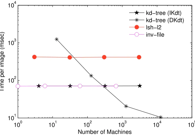
31

Figure 3.2: Kd-Tree Parallelizations. (Left)Independent Kd-Trees (IKdt). The images are

divided onto the machines, which build independent Kd-Trees for the images they contain.

At query time, all the machines are searched in parallel. (Right) Distributed Kd-Trees

(DKdt). The root machine stores the top of the tree, while the leaf machines store the leaves of the tree. At query time, the root machine directs features to a small subset of the leaf machines, which leads to higher throughput. See Section 3.3.2

100 101 102 103 104 105

101 102 103 104

Number of Machines

Time per image (msec)

kd−tree (IKdt) kd−tree (DKdt) lsh−l2

inv−file

Figure 3.3:Parallelization Run Time. Time per image vs. min. no. of machines required

M for different dataset sizes. Each point represents a dataset size from 106 to 109 images,

(48)

More sophisticated parallelization techniques are possible, that can take advantage of

the properties of the method at hand. For example, in the case of Kd-trees, one such

ad-vanced approach is to store the top part of the Kd-tree on one machine, and divide the

bottom subtrees across other machines (see Figure 3.2). We call this approach Distributed

Kd-Trees (DKdt), since different parts of the same Kd-Tree are distributed among different

machines. For 1012 features (109 images), we have 40 levels in the Kd-tree, and so we

can store up to 30 levels in onerootmachine, and split the bottom 10 levels evenly across

theleaf machines (see Section 3.4). Given a probe image, we first query the root machine

and get the list of branches (and hence subtrees) that we need to search with the

backtrack-ing. Then the appropriate leaf machines will process these query features and update their

ranked list of images.

The motivations for this distinction between root and leaf machines are:

• Most of the storage for the tree is in the leaves. Therefore we can store most of the

top of the tree in a single machine, which will then dispatch jobs to the leaf machines.

• The time spent searching the top of the tree is smaller than that spent searching the

lower parts of the tree, so we can gain more speed up by splitting the bottom part of

the tree instead of splitting the whole tree.

• Searching the tree will generally not activate all of the leaf machines, i.e., the list of

explored nodes will not span all the node machines. Therefore, the root machine can

process more features, and the leaf machines can interleave computations of

differ-ent features simultaneously. This offers more speed up over the first parallelization

(49)

33

first case, interleaving computations will make this much smaller.

This approach has the advantage of significant speed up and better utilization of the

ma-chines, since not all the machines will be working on the same query feature at the same

time, rather they will be processing different features from the probe image concurrently

(see figure 3.3). However, a drawback with this approach is the extra storage requirements,

because the lower parts of the trees will generally not store the same features for different

trees, and therefore each machine will have to store the features in the subtrees it is holding,

and as an upper bound the extra storage will be proportional to the number of Kd-Trees,

i.e., we will need to store each featureKtimes, whereKis the number of trees. We provide

more details on the implementations of Independent and Distributed Kd-Trees in Chapter

7.

Figure 3.2 shows a schematic of the Distributed Kd-Trees compared to the Independent

Kd-Trees, while Figure 3.3 shows the time per image vs. the minimum number of machines

Mfor different dataset sizes from 106to 109. We note the following:

• Distributed Kd-Trees provide significant speed ups starting at 108images. It might

seem paradoxical that increasing the dataset size decreases the run time, however

it makes sense when we notice that adding more machines allows us to interleave

processing of more features concurrently, and thus allows faster processing. This

however comes at a cost of more storage used (see Figure 3.3).

• We also note that many of the FR methods have parameters that affect the trade

off between run time and accuracy, e.g., number of hash functions or bin size for

(50)

and we should not use the same settings when enlarging the database. This poses a

problem for these methods, which have to be re-tuned as the database size changes,

as opposed to Kd-Trees which adapt to the current database size and need very little

tuning.

3.4 Theoretical Derivations

3.4.1 Exhaustive Search

Description

• Here we do the nearest-neighbor search using exhaustive linear search through the

set of database features {{fi j}j}i, i.e., for every feature of the query imagefq j, we

find the feature that minimizes the Euclidean distance: nq j =argmini jfi j, wherenq j

is the index of the feature andiis the image in the database containing this feature.

• For every database image, we count the number of such nearest neighborssi, and for

all images with a pre-set amount of nearest neighbors (10 in our experiments), we do

the RANSAC affine step to obtains′_iwheres′_i=# inliers of the affine transformation.

Storage

The storage requirements for this method are just the full feature vectors and feature

information:

• Feature vectors:

(51)

35

where s is the number of bytes per feature dimension, d is the dimension of the

feature vector,Iis the number of images in the database, andFis the average number

of features per image.

• Feature information:

Sf i=4IF

where for every feature we need to store its location (x and y position in the image)

in addition to its scale and orientation. We assume we can discretize this information

and fit it into 1 byte each.

• Total:

Sexhaustive= (sd+4)IF

Speed

• The main bottleneck is the nearest neighbor search. For every feature, we have to

search through the whole feature database to find the nearest feature:

Tnn,ex=F(2FId+FI) =F2I(2d+1)

where for every query feature we need to performd multiplications andd additions

per database feature, in addition to finding the minimum value amongFIvalues.

Parallelization

(52)

simul-taneously.

• Every machine processes the images it is storing, and produces a final sorted list of

geometrically checked images. This list is then broadcast or sent to a central machine,

which will merge them into one list and returns the result.

• Speed up: Having more machines here corresponds to linear speed up of the search

process (in the number of images). Consider havingMmachines, then each machine

will perform

T_nnp_,_ex= F

2_I

M (2d+1) +L(M−1)

where the second term is the time to mergeMsorted lists of lengthL.

3.4.2 Kd-Trees

Storage

• We still need to store all the features and their information:

Sex= (sd+4)IF

• In addition, there is storage for the trees. For a tree withnleaves, there are 2n−1 total

(53)

37

Storage for each tree is

Str = 2IF+IF

⌈log₂IF⌉

8

Str = IF(2+

⌈log₂IF⌉

8 )

where the first term is for the internal nodes where we need to store the dimension

and the threshold values (assumed to be discretized to single bytes), and the second

term is for the leaves where we need to store the index of the feature it contains

• Total:

Skdt = Sex+T Str

Skdt = IF(sd+4+2T+T

⌈log₂IF⌉

8 )

Computational Cost

• Searching through the Kd-Trees involves comparison operations at each level of the

tree, in addition to exhaustive search with the final list of features, typically ~ 250,

corresponding to the number of backtracking steps:

T_nn_,_kdt =FB(2d+1+log₂FI)

where the second term is for finding the minimum among theBdistance values, while

(54)

Parallelization

There are two ways to parallelize Kd-Tree operations. The first is a straightforward

extension of the exhaustive search case:

• Divide the data intoM machines. For every query feature, search the machines

si-multaneously.

• Combine the search results as for the exhaustive case, by having a local sorted list

of images, and then broadcast these lists to get a global sorted list, which is then

geometrically verified.

• Speed up: having more machines here corresponds to logarithmic speed up of the

search process. Consider havingMmachines, then each machine will perform

T_nnp_,_kdt=F(2dB+B+Blog₂FI

M) +L(M−1)

where L is the size of the list on each machine, and the second term is the time

required to mergeMsorted lists of sizeL.

The second is:

• Instead of having independent Kd-Trees in each machine, there will be a single (or

multiple) root machine with copies of the top part of the Kd-Trees. For example,

with 50 GB of memory available, we can fit 25 billion internal nodes. Therefore,

for storing 4 trees, we need to store ~ 6 billion nodes per tree (i.e. 3 billion leaves),

(55)

39

• The rest of the trees are then divided to the rest of theM machines (calledleaf

ma-chines) that will also store the feature vectors and information.

• The root machine(s) will get query features and compute an initial list of nodes to

explore based on the top of the tree. Then, it will dispatch that feature to all leaf

machines that have that part of the tree. Once a leaf machine gets a feature, it will

handle backtracking within its own subtree, and updating its ranked list of images.

• Speed up: We have two parts for the running time, one in the root machine and one

in the leaf machines:

T_nnp_,_kdt_,_r = FBlog₂ C

2×2T

T_nnp_,_kdt_,_l = FB

M (2dB+B) +Flog2

4FIT

C +L(min(FB,M)−1)

whereC is the memory capacity of each machine,T_nnp_,_kdt_,_r is the time to search the

root machine andT_nnp_,_kdt_,_lis the time for the leaf machines. The first term is the time

taken to search all theF image features concurrently where each feature will be sent

to at most Bmachines (and so we need FB machines to process them in the worst

case, where each backtracking step goes to a different leaf machine), the second term

is the time to get the minimum, the third term is the time to go down the subtree

excluding the top part in the root machine, and the last term is the time to merge the

(56)

3.4.3 Locality Sensitive Hashing (LSH)

Storage

Sex= (sd+4)IF

• In addition, there is storage for the tables. In each table, we need to store the hash

functions, in addition to the indices of all the features available:

Sta = IF

log₂IF

8 +Sh

where Shis the storage for the hash functions, which depends on the specific hash

function used and is negligible compared to the first term.

• Total:

Slsh = Sex+T Sta

S_lsh = IF(sd+4+T⌈log2IF⌉

8 )

Computational Cost

Searching through the LSH index involves computing the hash function values and then

(57)

repre-41

sented as

Tnn,lsh=F(Th+ (2d+1)

FI B T)

where the first term is the time to compute the hash functions:

• L2: Th,l2=T H(2d+2)where we haveH hash functions, and for each we need to

compute dot product (one addition and multiplication per dimension) plus another

addition and division.

• Spherical-Simplex: Th,sim=T H(2d(d+1) +d) =T H(2d2+3d)where we need to

compute product of ad+1×d matrix and a vector ofd dimensions, and then need

to get the closest vertex.

• Spherical-Orthoplex: Th,orth =T H(2d2+2d) =2T H(d2+d) where we need to

multiply ad×d matrix with advector, and then choose the nearest vertex from the

2dchoices, where we know that one vertex is just the opposite sign of the other.

The second two terms above are the time to compute exhaustive nearest neighbors, and

depends on the size of the LSH bucket, which is not constant, and grows linearly with the

number of total features, in addition to it varying greatly for the same number of features.

We assume we have a preset number of unique bucket valuesB, and then the average bucket

size would be FI_B.

Parallelization

There are two ways to parallelize LSH operations. The first is a straightforward extension

(58)

si-multaneously.

• Combine the search results as for the exhaustive case.

• Speed up: having more machines here corresponds to linear speed up. Consider

havingMmachines, then each machine will perform

T_nnp_,_lsh≈F FI

MBT(2d+1) +L(M−1)

The second is similar to Kd-Trees:

• Instead of having independent LSH indexes in different machines, there will be a

cen-tralmachine that computes all the hash functions, and has a list of which machines

store which buckets.

• The rest of the machines will store features that belong to a subset of buckets.

• The central machine(s) will get query features, compute the hash values (buckets),

and then dispatch that feature to machines containing that bucket.

• Speed up: We have two parts for the running time, one in the central machine and

one in the node machines:

Sm2,c = FTnn,lsh,x

Sm2,n =

F

T((2d+1) FI

(59)

43

whereSm,cis the time to compute the hash values on the central machine, whileSm,n

is the time taken for the node machines to search that bucket. This method will work

ifSm2,cis much smaller compared toSm2,n. On the other hand, it will be a bottleneck

if the two times are comparable.

3.4.4 Hierarchical K-Means (HKM)

Storage

Sex= (sd+4)IF

• In addition, there is storage for the clustering tree. For a tree with depth D and

branching factor k, there are kD leaf nodes, which will store the actual features (in

subsets ofk). The number of internal nodes is

n=

D−1

∑

i=0

ki= k

D₋₁

k−1

and for each internal node we need to store the kcluster centers, therefore the total

storage is

Shkm =

kD−1

k−1 ×ksd+ (sd+4)IF

(60)

• At each level of the clustering tree, we need to find the nearest cluster, in addition to

finding the nearest feature in the leaf node:

Tnn,hkm=F(D×(2d+k) +

FI

kD×(2d+1))

where the second term comes from searching the features in the leaf node, assuming

each leaf node will have the same share of features.

Parallelization

There are two ways to parallelize HKM operations. The first is a straightforward

exten-sion of the exhaustive search case:

si-multaneously.

• Combine the search results as for the exhaustive case.

• Speed up: Having more machines here corresponds to less search time. Consider

havingMmachines, then the each machine will perform

T_nnp_,_hkm=FD(2d+k) + F

2_I

MkD×(2d+1) +L(M−1)

The second is similar to Kd-trees:

• Instead of having independent HKM trees in different machines, there will be a

(61)

45

• The rest of the machines, node machines, will store subsets of the leaf nodes and

their features.

• The central machine(s) will get query features, go through the top of the tree, and

then dispatch features to the appropriate node machines.

• Speed up: We have two parts for the running time, one in the central machine and

one in the node machines:

Sm2,c = D(2d+k)

Sm2,n = 2d×

FI kD

whereSm,cis the time to go through the top of the HKM tree on the central machine,

whileSm,nis the time taken for the node machines to search the leaf nodes.

3.4.5 Inverted File (IF)

Storage

• We need to store the feature information (e.g., location) to allow the spatial

consis-tency step afterwards:

Sf i=4FI

• We also need storage for the inverted file:

Si f =W sd+FI(

log₂I

(62)

where the first term is the storage for theW words, and the second term is storage for

the lists of images. We have a total ofFI features and for each we need to store the

image id and the feature count.

• For large dictionaries of visual words, ~ 1 M visual words, image histograms tend to

be binary (i.e. there is one-to-one mapping between features and visual words) so we

do not need to store counts:

Si f,bin=W sd+FI

log₂I

8

• Total:

St = Si f+Sf i

= 4FI+W sd+FI(log2I

8 +1)

= W sd+FI(5+log2I

8 )

St,bin = W sd+FI(4+

log₂I

8 )

Computational Cost

There are two components for the run time

Searching Large Scale Image Collections