Scalable Loss-calibrated Bayesian
Decision Theory and Preference
Learning
M. Ehsan Abbasnejad
A thesis submitted for the degree of
Doctor of Philosophy at
The Australian National University
Declaration
I hereby declare that this thesis is my original work which has been done in collabo-ration with other researchers. This document has not been submitted for any other degree or award in any other university or educational institution. Parts of this thesis have been published in collaboration to other researchers in international conferences as listed below:
• (Chapter 3)E. Abbasnejad, S. Sanner, E. V. Bonilla, P. Poupart, Learning Community-based Preferences via Dirichlet Process Mixtures of Gaussian Pro-cesses,In Proceedings of the 23rd International Joint Conference on Artificial Intelli-gence (IJCAI), 2013. Beijing, China.
• (Chapter 4) E. Abbasnejad, E. V. Bonilla, S. Sanner, Decision-theoretic Spar-sification for Gaussian Process Preference Learning, Proceedings of the Machine Learning and Knowledge Discovery in Databases - European Conference (ECML PKDD), 2013. Prague, Czech Republic.
• (Chapter 5) E. Abbasnejad, J. Domke, S. Sanner, Loss-calibrated Monte Carlo
Action Selection, In Proceedings of the 26th Conference on Artificial Intelligence (AAAI), 2015. Austin, USA.
M. Ehsan Abbasnejad April 26, 2017
Acknowledgments
I would like to express my gratitude towards all who helped me make this thesis possible.
First and foremost, I wish to thank my supervisorScott Sanner for all his guid-ance, caring and patience and providing me with the excellent atmosphere for doing research. Scott’s intuitive understanding of Bayesian methods and decision theory motivated my research and gave me insights that would have never been possible without him. His encouragements have been invaluable to me during the hard times. I am extremely grateful for his strong support in my academic and personal life. I also wish to thank my advisor Edwin V. Bonilla, who gave me the opportunity to learn Gaussian processes. Special thanks to Justin Domke whose advice on math-ematical formulation and problem solving has been invaluable. His deep and intu-itive understanding has been a great help and motivation. I would like to express my warm respects towardsMark Reidas my advisor, for his time and helpful sug-gestions. I would also like to thankPascal Poupartwho gave me a better insight into Nonparametric Bayesian methods during my visit. I am eternally in debt to these academic role models.
I acknowledge the financial, academic and technical support provided by the National ICT of Australia (NICTA) and the Australian National University (ANU) and thank them for their support in my research. My fellow postgraduate friends at NICTA and the ANU provided a welcoming collaborative environment. I would like to specially thank Zahra Zamani, Alireza Motevalian, Sarah Taghavi Namin, Mohammad Ismailzadeh, Mohammad Najafi, Ehsan Nabavi, Hadi Afshar, Behrouz Nasihatkon, Salim Masoumi, Alireza Khosravian, Mehdi Shabani, MohammaReza Jouyandeh, Fateme Rajabi, Morteza Azad, Sahba Najafi, Mohsen Zamani, Mona Golestar Far, Suvash Sedhain and many others who always cheered me on and made my life so joyful.
Finally I have to thank my parents who have always supported me and gave me the encouragement to follow my dreams. I thank them for believing in me and for their endless love and support. My brothers, Iman and Amin, I thank you for always being my best friends and supportive of whatever I have done.
Above all I wish to thank the almighty God for his guidance in life and giving me the opportunity to pursue my degree.
Abstract
Bayesian decision theory provides a framework for optimal action selection under uncertainty given a utility function over actions and world states and a distribution over world states. The application of Bayesian decision theory in practice is often limited by two problems: (1) in application domains such as recommendation, the true utility function of a user is a priori unknown and must be learned from user interactions; and (2) computing expected utilities under complex state distributions and (potentially uncertain) utility functions is often computationally expensive and requires tractable approximations.
In this thesis, we aim to address both of these problems. For (1), we take a Bayesian non-parametric approach to utility function modeling and learning. In our first contribution, we exploit community structure prevalent in collective user prefer-ences using a Dirichlet Process mixture of Gaussian Processes (GPs). In our second contribution, we take the underlying GP preference model of the first contribution and show how to jointly address both (1) and (2) by sparsifying the GP model in order to preserve optimal decisions while ensuring tractable expected utility compu-tations. In our third and final contribution, we directly address (2) in a Monte Carlo framework by deriving an optimal loss-calibrated importance sampling distribution and show how it can be extended to uncertain utility representations developed in the previous contributions.
Our empirical evaluations in various applications — including multiple prefer-ence learning problems using synthetic and real user data and robotics decision-making scenarios derived from actual occupancy grid maps — demonstrate the effec-tiveness of the theoretical foundations laid in this thesis and pave the way for future advances that address important practical problems at the intersection of Bayesian decision theory and scalable machine learning.
Contents
Declaration 3
Acknowledgments 7
Abstract 9
1 Introduction 1
1.1 Motivation . . . 1
1.2 Basic Framework . . . 3
1.3 Contributions . . . 4
1.4 Thesis Outline . . . 5
2 Background 7 2.1 Foundation of Decision Theory . . . 7
2.1.1 Basic Definitions . . . 7
2.1.2 Modeling Uncertainty . . . 9
2.1.2.1 Graphical Models . . . 9
2.1.3 Using Prior and the Bayesian View . . . 10
2.1.4 Bayesian Decision Theory . . . 13
2.2 Bayesian Modeling and Learning . . . 14
2.2.1 Parametric Bayesian Modeling . . . 14
2.2.2 Nonparametric Bayesian Modeling . . . 16
2.2.2.1 Gaussian Processes . . . 17
2.2.2.2 Dirichlet Processes . . . 20
2.3 Bayesian Inference . . . 22
2.3.1 Laplace Method . . . 22
2.3.2 Variational Inference . . . 23
2.3.3 Expectation Propagation (EP) . . . 24
2.3.4 Sampling and Markov Chain Monte Carlo (MCMC) . . . 26
2.3.4.1 Monte Carlo Methods . . . 26
2.3.4.2 Gibbs Sampling . . . 27
2.3.4.3 Metropolis-Hastings . . . 28
2.4 Bayesian Decision Theory and Preference Learning . . . 29
2.4.1 Preferences and Existence of the Utility . . . 29
2.4.2 Risk-seeking vs. Risk-averse Behavior . . . 31
2.4.3 Learning the Utility Function . . . 31
3 Learning Community-based Preferences 35
3.1 Gaussian process for Multi-user Preference Learning . . . 36
3.1.1 Prediction . . . 39
3.1.2 Optimizing the Kernel Hyper-parameters . . . 40
3.2 Dirichlet Process Mixtures of Community-based Preference GPs . . . . 40
3.2.1 Inferring Community utilities . . . 42
3.2.2 Inferring Community Membership . . . 44
3.2.3 Prediction . . . 45
3.2.4 Final Algorithm . . . 46
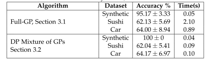
3.3 Empirical Evaluation . . . 46
3.4 Related Work . . . 50
3.5 Conclusion . . . 50
4 Decision-theoretic Sparsification for Gaussian Process Preference Learning 51 4.1 Decision-theoretic Sparsification . . . 52
4.1.1 Observation-driven Sparsification . . . 52
4.1.2 Item-driven Sparsification: Valuable Vector Machine . . . 53
4.1.3 Loss Functions and Risk . . . 55
4.1.3.1 Log loss and IVM . . . 55
4.1.3.2 Valuable Vector Machine – Value Of Information . . . . 55
4.1.3.3 Valuable Vector Machine – Upper Confidence Bound . 55 4.2 Empirical Evaluation . . . 56
4.2.1 Datasets . . . 58
4.2.2 Results . . . 59
4.3 Related Work . . . 60
4.4 Conclusion . . . 61
5 Loss-calibrated Monte Carlo Action Selection 63 5.1 Loss-calibrated Monte Carlo Importance Sampling . . . 65
5.1.1 Minimizing regret . . . 66
5.1.2 Minimizing the probability of suboptimal action . . . 67
5.1.3 Optimalq . . . 71
5.2 Applications . . . 73
5.2.1 Power-plant Control . . . 73
5.2.2 Robotic Navigation . . . 76
5.3 Conclusion and Future Work . . . 77
6 Conclusion 79 6.1 Summary of Contributions . . . 79
6.2 Future Work . . . 80
Contents 13
A Alternative Formulation of the Loss-calibrated MC Action Selection 85
List of Figures
2.1 A graphical model of three random variables x1,x2,y . . . 9
2.2 Graphical model and the plate representation . . . 11 2.3 Hierarchical Bayesian model . . . 13 2.4 Bayesian linear regression: the prior and the posterior of the parameter
θare shown in Figure 2.4(a). In Figure 2.4(b), the dots are the observed points. The red lines are three samples from the linear function defined by the posterior distribution. As is shown, the posterior is peaking at the true value (1 in this example). . . 15 2.5 Graphical model of the Mixture Model . . . 16 2.6 Dirichlet distribution for various values of α . . . 20
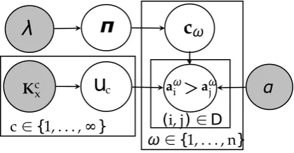
2.7 An illustration of the Dirichlet distribution and the partitioning of the space. . . 21 2.8 A graphical model for EP . . . 25 3.1 Our proposed generative graphical model for community-based
pref-erences. There is a plate for users ω with community membership
indicator cω ∈ C and an embedded plate for i.i.d. preference
obser-vations aω
i aωj of user ω depending on the community assignment
cω of ω, community cω’s latent utility function ucω, and the
discrim-inal dispersion parameter α. There is a separate plate for
commu-nities c ∈ C = {1 . . . ,∞} which contains the latent utility function
uc drawn from a Gaussian Process conditioned on local (optimized) community parameters Kcx. Finally, each cω is generated i.i.d. from
an infinite multinomial distribution with parameters π and Dirichlet Process prior with concentration parameter λ. . . 41
3.2 The distribution of preferred cars in each community for the AMT car dataset. Each x-axis position represents a different car and the y-axis the normalized frequency with which that car was preferred to another by a user in the community. Each community is distinct and differs in at least one car attribute. . . 48 3.3 Distribution of communities in the datasets . The x-axis is the number
of communities; the y-axis is the posterior probability at the last sam-pling iteration. These values are obtained at iteration 15 of Synthetic and Sushi and iteration 36 of AMT Car. . . 49
4.1 Illustration of Value of Information: it is the product of the shaded area under the normal curve when the utility is higher than the opti-mal value and the linear function of their difference. This value cor-responds to the expectation of the difference of the utility of the item and the optimal under the shaded mass. As it is observed, uω
1 has
negligible mass above uω,∗ point, therefore the item corresponding to uω
2 is selected. . . 56
4.2 Performance of the sparsification methods in terms of the recommen-dation loss (the proportion of items that are incorrectly predicted as the best item for recommendation) in the first column and the 0/1loss
(percentage of wrongly predicted preferences) in the second, as a func-tion of the proporfunc-tion of items selected for sparsificafunc-tion. The larger the number of items the lower the level of sparsification and the closer the algorithms are to the Full-GP method. . . 57 4.3 Average prediction time for inference with 200 users and 10 items. The
number calculated as the time consumed to make a series of predic-tions on the preferences of the test set. . . 60 5.1 Motivation for loss-calibration in Monte Carlo action selection. (Top) Utility
u(θ)for actionsa1anda2as a function of stateθ. (Middle) A belief state
dis-tributionp(θ)for which the optimal action arg maxa∈{a
1,a2}Ep[u(θ,a)]should
be computed. (Bottom) A potential proposal distributionq(θ)for importance
sampling to determine the optimal action to take inp(θ). . . 64 5.2 Power-plant simulations: the step-valued utility function (as in
Equa-tion 5.17 and 5.18) in the first column, the true distribuEqua-tion p (in blue) and q∗ (in red) in the second column and in the third and forth columns the result of performingSubsampled MCandMultiple MC(as de-scribed in the text) are shown. In the two right-hand columns, note that q∗ achieves the same percentage of optimal action selection per-formance as pin a mere fraction of the number of samples. . . 75 5.3 Performance of the decision maker in selecting the best action as the
dimension of the problem increases in the power-plant. Note that at 100 dimensions, pis unable to select the optimal action whereasqstill manages to select it a fraction of the time (and would do better if more samples were taken). . . 76 5.4 A robot’s internal map showing the samples taken from its true belief
distributionp(two modes are shown in blue, the second one is slightly obfuscated by the robot) and the optimal sampling distributionq∗ de-rived by our loss calibrated Monte Carlo importance sampler in 5.4(a). In 5.4(b) and 5.4(c) we see the performance (in terms of percentage of optimal action selected) of our loss-calibrated sampling method using
Chapter1
Introduction
1.1
Motivation
Every day, people and computers are faced with decision making in uncertain cir-cumstances. Decision theory is the study of optimal decision making under uncer-tainty. It is concerned with the analysis of the consequence ofactionsin an uncertain environment. Decision theory requires three major components: state,action,and the
utility function. The utility function is a means of evaluating how valuable an action (i.e. a choice amongst alternatives) is for the decision maker in a given state of na-ture. The expectation of this utility for an action with respect to the uncertain states is theexpected utilityand maximizing it is the core focus of decision theory.
In this formulation, conventional decision theory assumes the utility is known to the decision maker. However, in many applications this assumption is not valid. The utility may only be formulated by or revealed to the decision maker through an interaction with the environment and may be partially known. Consider the following examples:
• Recommendation: The objective of a recommender system is to suggest
attrac-tive items (alternaattrac-tives) to the users that potentially leads to their selection (e.g. purchase). With an abundance of consumer choices, such systems are becoming increasingly popular to direct users to what they might find useful. One way these recommenders provide these suggestions is by learning from the users’ feedback that was collected from their previous preferences for items. Under certain assumptions, we can model preferences using utilities. These utilities are unknown and user’s preferences provide information to help formulate belief about their true values.
• Robotic automation: Navigation and exploration are vital tasks in robotics
and entail making choices amongst a variety of alternatives. For example an unmanned aerial vehicle (UAV) for scientific research has to maximize area covered while choosing a path, places to stop for observation, duration of stay while observing, and types of measurements [28]. These all have to be done while carefully avoiding collisions with other objects, such as moving UAVs [5]. Also, one has to consider the fact that certain actions might perform well for a mission and poorly for others. Manually determining the utility function needs
a tedious investigation into the mission, the field, and possible consequences of each action. Alternatively, learning it (or improving from what was learned in a similar mission) through the collection of information from the environment can be considered.
• Automated medical assistant: Assessing the effectiveness of a medical
treat-ment is generally hard and has to be tailored towards the needs of each indi-vidual patient [22]. This is because each patient might feel differently about the process and consequences of each treatment. For instance, one might prefer a short but intensive treatment over a longer, relatively comfortable one. By presenting these alternatives at a given stage to a patient we can construct a personal utility function. We might start with a “general” utility function as a prior and update it as patient’s preferences are observed. In this process, we learn the utility of each patient during the course of a treatment.
• Autonomic computing: Managing a cluster server can be a tedious and
error-prone task. It can ideally be managed automatically by the computers them-selves with minimal human intervention [16, 66]. These systems are becom-ing crucial due to the increasbecom-ing popularity of cloud computbecom-ing where users can run their programs on these cloud resources and pay accordingly. An au-tonomic system seeks to maximize its income by intelligent allocation of all resources while ensuring certain quality constraints (such as maximum wait time in the queue) are satisfied. The utility function measures how much the allocation of a resource (e.g. CPU) to a task in the queue earns for the cloud service provider while maximizing the customer’s satisfaction. This utility is unknown in advance because each application’s resource requirements are not known and different. Learning the utility of resources for each application ensures a better allocation and consequently a better quality of services. In all these examples, the utility function is initially unknown or imprecise. The value of utilities is inferred from some form of available information (e.g. prefer-ences). With observing the alternative choices and their consequences, we formulate a "belief" in a utility function. For example in a recommender system, observing a purchase of a comedy movie increases the certainty that the user is interested in this genre and may assign higher utility values to instances of such movies.
§1.2 Basic Framework 3
Once the utility is formulated, finding the action to be performed requires calcu-lation of expected utilities that leads to computationally expensive integrals. This is true if either the utility is manually formulated or learned using probabilistic model-ing methods. Efficient computation of the expected utility is a challengmodel-ing problem that we also investigate in this thesis. In the subsequent section, we provide a more formal description of the fundamental problems that we address in this thesis.
1.2
Basic Framework
Bayesian theory [7, 32, 77] provides a formalization of robust decision-making in uncertain settings by maximizing expected utility. Formally, a utility func-tion u(θ,a) quantifies the return of performing an action a ∈ A = {a1, . . . ,ak} in a given state θ. When the true state is uncertain and only a belief state distribu-tion p(θ) is known, Bayesian decision-theory posits that an optimal control actiona should maximize theexpected utility
EUu(a) =Eθ∼p(θ)[u(θ,a)] =
Z
u(θ,a)p(θ)dθ, (1.1) where by definition, theoptimal action a∗ is
a∗ =arg max
a EUu(a). (1.2)
This conventional formalization assumes the utility is given and completely known. As discussed earlier, this is not always the case and utilities can be unknown or im-precise in various applications. Since we are treating the utility function as a random quantity, we have a belief in its values (technically a random function). Therefore, we are led to the framework known asexpected expected utility[15] that takes an expecta-tion both over state and utility uncertainty:
EEU(a) =Eu∼p(u)
EUu(a)
=
Z
EUu(a)p(u)du. (1.3)
Hereuis a functional andp(u)is a distribution over this functional. As expected, the optimal action is the one that maximizes this expression. For a fully known utility function, that is when the distribution of the utilities is a Dirac delta function centered at this fixed utility, we recover the conventional decision theoretic framework given in Equation 1.1.
When there is no observation in the Bayesian modeling of p(u), the utility value is represented in the prior provided by the expert. As more observations become available, the belief in the utility is updated.
• Learning a distribution over utility functions: In practice, modeling the dis-tribution of the utility function itself is difficult. For instance, utilities have to be inferred from pairwise comparisons in preference learning. Then the first question is how to learn a utility belief model p(u)from observations?
• Efficient computation of the optimal action: Once the utility is learned, finding the optimal action is often expensive and needs an efficient computation of the integral in the expected utility. In this case, if we are given a fixed utility, how do we efficiently compute EUu(a)? On the other hand, if we have a distribution over the utility p(u), then how to compute EEU(a)?
These two issues are the main problems that will be addressed in this thesis.
1.3
Contributions
As outlined previously, the two aims of this thesis are learning a distribution over utility functions and efficient computation of the optimal action. As such, in the following we summarize our main contributions:
• Learning Community-based Preferences via Dirichlet Process Mixtures of
Gaussian Processes: To formulate our belief in a utility function, we need a
flexible model that requires minimal constraints on the structure of utilities. This model has to be able to automatically adapt to the amount of data. Our first contribution is to use nonparametric Bayesian methods, in particular Gaus-sian Processes (GPs) [74], to model the distribution of the utility. However, as these models can grow prohibitively large when numbers of users grow, we leverage the notation of communities to motivate nonparametric clusterings of users for an efficient representation. This efficient extension reduces cubic op-erations for computing the posterior to linear ones using the Dirichlet Process (DP) [85]. We provide an application of this method to preference learning and show that our proposed approach is capable of grouping users based on their preference clusters.
• Decision-theoretic Sparsification for Gaussian Process Preference Learning:
§1.4 Thesis Outline 5
• Loss-calibrated Monte Carlo Action Selection: Obtaining the optimal action
that maximizes the expected utility requires computationally expensive inte-grals typically evaluated using Monte Carlo methods in both conventional Bayesian decision theory in Equation 1.1 and EEU in Equation 1.3. We provide an improved Monte Carlo method to find the optimal action in a fraction of the time compared to its conventional counterpart; To do this, we use the calculus of variations to find the optimal distribution that minimizes theregret, that is, we minimize the probability of suboptimal action selection when the number of samples is limited. As will be shown, this objective further minimizes the probability of suboptimal action selection in the finite sample case.
Putting these three basic contributions together we lay the foundation for efficient and scalable computation of expected expected utility for optimal Bayesian decision-theoretic action selection. Our empirical evaluations in various applications — in-cluding multiple preference learning problems using synthetic and real user data and robotics decision-making scenarios derived from actual occupancy grid maps — demonstrate the effectiveness of the theoretical foundations laid in this thesis and pave the way for future advances that address important practical problems at the intersection of Bayesian decision theory and scalable machine learning.
1.4
Thesis Outline
Chapter2
Background
As explained earlier in the introduction, decision theory studies models of decision making for agent(s) under Bayesian models of environment uncertainty. In this sec-tion we will provide the background material needed for our contribusec-tions in the rest of this thesis. In particular, we will discuss:
• What is decision theory and how it is formally defined? How can we model the uncertainty involved in the decision making process? We will formally introduce decision theory in Section 2.1 and modeling uncertainty in Section 2.1.2
• Amongst the decision theoretic frameworks, Bayesian decision theory is a com-pelling choice because it models the uncertainty as an explicit probability dis-tribution and, as will be argued in Section 2.1.4, is the framework that we will focus on. Since we will be using Bayesian decision theory, we will discuss its differences with the frequentist’s view. We further discuss how the Bayesian models are built and used for learning and inference in Section 2.2. In Section 2.3 we will provide some remarks on approximate Bayesian inference.
• Finally we draw the connection between the Bayesian decision theory and pref-erence learning via a notion of a utility function in Section 2.4.
2.1
Foundation of Decision Theory
In this section we will explain the basics of decision theory. Further reading on decision theory can be found in [7–9, 77][45, Chapter 22][31, 32, Chapter 9].
2.1.1 Basic Definitions
In this thesis, we use a decision making scenario consisting of three basic elements,
state, actionandutilityas detailed below:
• The state indicates the condition of the nature that the decision maker is in and is typically not fully realized and thus uncertain. This uncertainty can be due to the changing nature of the decision maker’s environment or the noisy tools
for measurement. As such, the “belief” over the value of the state is typically conditioned on some observations. This uncertain variable, denoted asθ ∈ Θ (depending on the application can be vector of continuous or discrete values), describes the attributes of this environment. When experiments are performed to gather information about the value of θ, it is called the parameter in some parameter space. We use the state of nature and the parameter interchangeably to refer toθ.
• The decision maker can affect its environment by taking an action a ∈ A in the set of all possible actions under considerationA={a1,a2, . . . ,ak}. At each state, the action performed produces an outcome o : A ×Θ. The analysis of this outcome for the selected action is of central interest to decision theory. • The utility function is a means of evaluating how valuable the outcome of an
action is for the decision maker in a given state. This functionu :Rd× A →R returns higher values for the actions that are more favorable in a given state. In the cases where there is no uncertainty (i.e. deterministic environment), the optimal action is the one that has the highest utility. However, in general the environment is uncertain and we need to consider expected utility over all possible states. In some applications it is insightful to think of the utility value in a monetary manner although this is not always the case.
In this thesis, we assume the outcomeois deterministic on the state-action space and therefore the utility of the selected action in the given state u(θ,a) is equivalent to the utility of the outcomeu(o), i.e.u(o) =u(θ,a).
Given a distribution over the state of the nature and a utility function, we define theexpected utilityas:
EUu(a) =Eθ∼p(θ)
u(θ,a)
, (2.1)
with theoptimal actionbeing the one that maximizes this value, i.e.,
a∗= arg max
a EUu(a)
That is, with respect to our belief about the state of nature, the action that maxi-mizes the expected utility is optimal. This definition connects three basic elements of decision theory. In the following we further detail how to obtain and model the distribution of states and the utility.
§2.1 Foundation of Decision Theory 9
y
x
1x
2(a) Bayesian network
y
x
1x
2 [image:25.595.210.427.117.213.2](b) Factor graph
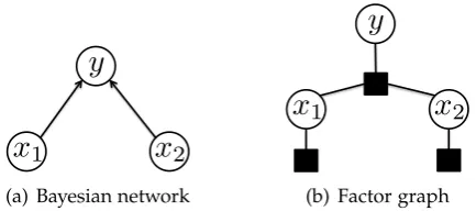
Figure 2.1: A graphical model of three random variablesx1,x2,y
2.1.2 Modeling Uncertainty
A well-understood mathematical tool for representing and reasoning under uncer-tainty is probability theory that is foundational to Bayesian methods that underly work in this thesis. In this section we discuss how to represent the probabilities and learn from observations. In subsequent sections where we discuss the uncertainty in the utility function, we employ the same modeling tools for the distribution of the utilities.
2.1.2.1 Graphical Models
Graphical models are the marriage of graph theory and probabilistic modeling. The reason for using such models is more compact representation of the joint probabilities by exploiting the independence of random variables. In particular for modeling the unknown state of nature, we might notice interactions among various variables that lead to a structured graphical model of conditional dependence. In addition, these graphical representations allow exploiting structure for efficient inference and paves the way for use of well-developed graph algorithms for probabilistic reasoning in graphical models. In short, we use a graph representation because:
• the graph structure reveals properties of the model, namely dependence/inde-pendence of variables;
• inference and learning can exploit the structure of graphical models for effi-ciency;
• much more compact than the explicit representation of full joint;
• compact models with fewer parameters have higher bias but can be learned with lower variance than full joint; and,
• it is easier to visualize the structure of the probabilistic models.
1. Undirected Graphical Models: Also known as Markov Random Fields (MRF),
represent the distribution that factorizes according to set of functions ψ that
define the interaction (or compatibility) between the variables in a clique. De-noting byC a clique in the graph, the joint probability of d random variables θ1, . . . ,θd, can be written as:
p(θ1,θ2, . . . ,θd) = 1
Z
∏
C ψC(θC),where θC is the subset of variables belonging to the clique C and their corre-sponding compatibility functionψC.
2. Directed Graphical Models: Also known as Bayesian networks, represent the
connection between variables in a parent-child relationship that is specified by the arrow direction in the graph. In this relation, the children depend on their parents. Therefore, the joint distribution factorizes based on the parents pa(θ) of a variableθ, that is,
p(θ1,θ2, . . . ,θd) =
∏
p(θi|pa(θi)).An example of a directed graph is shown in Figure 2.1(a). In this graph,x1,x2
are the parents ofy. The direction of arrows in the graph represent the direction of conditional dependency between variables. The joint in this figure represents the following:
p(x1,x2,y) = p(y|x1,x2)p(x1)p(x2)
Both directed and undirected graphical models can be easily depicted in a fac-tor graph as shown in Figure 2.1(b). The factor graph represents the factorization of a function. In a factor graph, the black squares represent the potential function between the connected random variables. This interaction is the compatibility func-tion in undirected graphs or the joint distribufunc-tion of the connecting variables in the directed one.
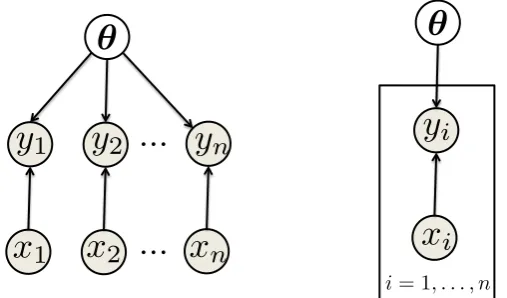
In many problems where the number of random variables is large and there are patterns of conditional independence, a plate diagram as shown in Figure 2.2 is conventionally used to provide a simpler representation. A simple example is shown in Figure 2.2 where variableyi depends onxi andθfor all i=1, 2, . . . ,n. The observed variables are normally shaded in graphical models. This graphical model is common in machine learning (regression and classification) where the target value (label) y depends on the observation x and the state of nature θ. We will discuss a regression example (whereyis continuous) in the following sections.
2.1.3 Using Prior and the Bayesian View
§2.1 Foundation of Decision Theory 11
x
1
✓
y
1
y
2
y
n
x
2
...
x
n
...
✓
x
i
y
i
[image:27.595.193.447.114.263.2]i= 1, . . . , n
Figure 2.2: Graphical model and the plate representation
• The frequentist view is that the state of nature is an unknown that we have measurements from. One formulates a hypothesis model that minimizes the average loss of the observed measurements. Through a large number of obser-vations, the model that minimizes the average loss on the training observations learns to recognize the unseen samples with a good performance. Similarly, models that find the single parameter that maximizes the probability of the observations are frequentist.
• The Bayesian view on the other hand, thinks of the state of nature as a random variable. Hence as a random variable, there is an initial belief about its value and upon seeing new observations this belief is updated. Bayesian modeling is done with the view that the uncertainty about the unknown state of nature is often reduced as more observations are made.
Bayesian methods use simple probability rules to infer unknown states. In particular, for two random variables AandB, we will use two standard probability rules:
p(A) =
Z
p(A,B)dB marginalization (sum/integrate out),
p(A,B) = p(A|B)p(B) chain rule (product rule).
These probabilistic principles combined with the basic Bayes rule lay the founda-tion for Bayesian reasoning about the uncertainty of the unknown state,
p(θ|D) = p(D|θ)p(θ)
Z , (2.2)
where Ddenotes the set of observed random variables{di}i=1,...,nand
Z = p(D) =
Z
distributed, the likelihood term factorizes, i.e.
p(D|θ) = n
∏
i=1p(di|θ)
In Figure 2.2, the graphical model of such factorization wheredi = (xi,yi)is shown. Here, p(θ)represents theprior, p(D|θ)thelikelihoodandZis the normalizer that ensures theposterior on the left-hand-side (LHS) sums to one, and hence is a proper distribution. This prior is obtained from a problem-specific expert’s knowledge or a similar problem. The distribution of the prior is often determined by its parameters that are called hyper-parameters to set apart from the unknown parameters we are looking for.Inferenceis the procedure of obtaining the posterior distribution of these unknown parameters from the prior using the likelihood. The posterior, p(θ|D), is the distribution of the state variable given the observations. When we are in the no-datasetting, that is, there are no observation, the posterior is equal to the prior. Upon having new observations we can incrementally update our belief about the state. In each step, the posterior of the previous iteration acts as a prior in the Bayes rule to update the belief aboutθ, i.e.
p(θ|D) ∝ p(dn|θ)p(θ|D1,...,n−1)
whereD1,...,n−1is the set of firstn−1 observations.
When the integral in the normalizer Zis tractable, exactinference can be carried out. Often times in practice however, the integral is hard to perform and as such var-ious sampling and approximation methods are developed to estimate the posterior. We will discuss these methods in the subsequent section.
An important advantage of Bayesian modeling is that, as opposed to the fre-quentest view,over-fittingorunder-fittingis automatically avoided. That is because in Bayesian methods, for prediction we integrate over all parameterizations, i.e.
p(d∗|D) ∝
Z
p(d∗|θ)p(θ|D)dθ
where d∗ is the unseen sample. This integration acts as an averaging with respect to all possible parameter values as opposed to picking the parameter that maximizes the posterior probability which might overfit the data and lead to poor generalization to unseen examples.
Furthermore, Bayesian models are generally considered consistent in the sense that if the true parameter valueθ∗ that generates the data is in the prior, as the num-ber of observations approach infinity, the posterior converges to the delta function centered at the true parameter value [31, 32], i.e., fornobservations inD,
lim
n→∞p(θ|D) → δ(θ−θ∗).
§2.1 Foundation of Decision Theory 13
✓
xi
yi
i= 1, . . . , n
Figure 2.3: Hierarchical Bayesian model
A Bayesian model can be hierarchical by having multiple levels of priors where priors of priors are hyper-priors:
p(θ) =
Z
p(θ|λ)p(λ)dλ.
where λ is the hyper-parameter. A graphical model of this new representation is shown in Figure 2.3. This will add further flexibility in the model. Although hierar-chical models are more complex and their inference is more challenging, in problems like topic modeling they proved to be effective [13].
2.1.4 Bayesian Decision Theory
Now that the state distribution in a Bayesian view can be obtained from the observa-tions, we can proceed to introduceBayesian decision theoryas:
EUu(a) =Eθ∼p(θ|D)[u(θ,a)] =
Z
u(θ,a)p(θ|D)dθ. (2.4) with theoptimal action a∗ being the one that maximizes this value, i.e.,
a∗= arg max
a EUu(a) Then actiona1ispreferredto actiona2if and only if
EUu(a1) > EUu(a2).
We say the decision maker isindifferentabouta1anda2when EUu(a1) =EUu(a2).
i.e.
EEU(a) = Eu∼p(u)
EUu(a)
=
Z
EUu(a)p(u)du.
Then the utility of an action is a distribution of the utility for that action and there is no independent state variable to consider.
2.2
Bayesian Modeling and Learning
So far we have introduced the general picture of decision theory without discussing the specific models. In this section, we concentrate on the Bayesian modeling for learning the distribution of unknown variables. These variables can be (1) the state of nature, (2) the utility function, or (3) otherlatentvariables that the belief over state or utility function depends on.
In Bayesian modeling, we choose the prior and the likelihood and compute the posterior from the Bayes rule. When the product of the prior and the likelihood re-mains in the same family, computing the posterior is tractable and the prior is called
conjugate. Formally, if M is a set of prior distributions onθ, then the prior is called conjugate to the likelihood model if for every observation, the posterior is inM. We will give an example of a tractable problem and then discuss various approximate methods that in subsequent chapters will be used for intractable problems.
In the following we will discuss parametric and nonparametric Bayesian models. A particular characteristic of the parametric Bayesian modeling is that there is a fixed dimensional parameter whose posterior distribution we are interested to obtain. The posterior in these models takes a fixed size parametric form. In the nonparametric models on the other hand, the dimension of the parameter can grow with the data. In the following, we will discuss them in details.
2.2.1 Parametric Bayesian Modeling
In the Bayesian view we are interested in the distribution of the unknown random variables. There is an initial belief about the value of these unknowns that ulti-mately become more certain with more observations. In case these likelihoods and the prior are conjugate we can compute the products in closed form and the integral is tractable. For example Gaussian distribution is a conjugate prior for a Gaussian likelihood as in theBayesian linear regressionbelow.
As an example of the parametric Bayesian modeling, consider the observations to be a set of pairs D = {(xi,yi)}ni=1 where xi ∈ Rd and yi ∈ R as a regression problem. The graphical model of this regression problem is shown in Figure 2.2 that corresponds to the following:
p(θ|D) = 1
Zp(θ)p(D|θ) =
1
Zp(θ)
n
∏
i=1§2.2 Bayesian Modeling and Learning 15
−6 −4 −2 0 2 4 6
θ
0.0 0.2 0.4 0.6 0.8 1.0 1.2
p
p(θ) p(θ|D)
(a) Prior and posterior on weights
1.0 1.2 1.4 1.6 1.8 2.0 2.2
x
0.5 1.0 1.5 2.0 2.5 3.0 3.5
y
[image:31.595.129.518.125.287.2](b) Regression model
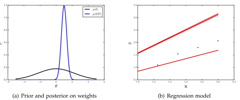
Figure 2.4: Bayesian linear regression: the prior and the posterior of the parameterθ are shown in Figure 2.4(a). In Figure 2.4(b), the dots are the observed points. The red lines are three samples from the linear function defined by the posterior distribution.
As is shown, the posterior is peaking at the true value (1 in this example).
In case of regression where we are not modeling p(xi), we can write the likeli-hood as p(yi|xi,θ) (i.e. since xi is observed, its distribution is absorbed in the nor-malizer). Assuming a Gaussian prior, θ ∼ N(0,α2Id) and a Gaussian likelihood yi ∼ N(θ>xi,β2Id)with hyper-parametersα,β∈R, the posterior is
p(θ|D) = N(β−2SX>y,S). S=α−2I+β−2X>X
−1 ,
whereId is the identity matrix of sized,Xis the matrix constructed from observation
x and y is the vector of labels. The posterior is a distribution over the value of the state of nature which represents the linear functions that generated the label y. Here, if the labels are binary (±1), the likelihood model is not Gaussian (i.e. not conjugate) and hence the integral in the posterior becomes intractable and requires approximation.
An illustration of this model at work is shown in Figure 2.4. The dots in Figure 2.4(b) represent the observations that are generated from a linear function with a small additional noise. That is, we chose a constant weight that was multiplied by each point on the x-axis and then a random noise was added to the output as shown in the y-axis, i.e. y∼ N(x>θ,β2). The prior, a zero mean Gaussian distribution over
that unknown weight, and the posterior that was obtained from these observations is shown in Figure 2.4(a) where the posterior is peaked at the true parameter value that generated the data. This posterior represents the belief over the space of weights that could generate the observations (with the given likelihood parameterβthat specifies
x
ii= 1, . . . , n
c= 1, . . . , m
✓
c [image:32.595.226.330.112.194.2]c
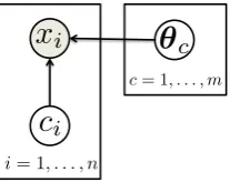
iFigure 2.5: Graphical model of the Mixture Model
posterior Gaussian distribution on the weight vectors becomes sharper and looks more like a delta function. It is an important example that shows how the conjugate likelihood can lead to an efficient inference. We will get back to this example again when we discuss Gaussian processes and Bayesian inference.
Bayesian parametric models can be used in the estimation of the mixture models as well. The easiest way to think about the mixture model is in clustering where a subset of observations form a group (k-means can be seen as a non-Bayesian mixture model). Instead of a labeled set, we have an unlabeled setD= {x1,x2, . . . ,xn}and a mixture model for the likelihood. That is, there is a parameter vector for each cluster and there is a hidden variableci that specifies which cluster each observationxi be-longs to. The likelihood of each observation given its cluster is p(xi|θc)(distribution of each observation depends on the parameter of that cluster). Then we have,
p(θ|D) = 1
Z
m
∑
c=1p(θc) n
∏
i=1p(ci = c)p(xi|θc). (2.5)
The integration of the posterior distribution becomes intractable in general and needs sampling or approximate inference. If we assumep(xi|θc)andp(θc)are conju-gates (say a Gaussian distribution like the regression problem), we can useExpectation Maximization (EM)to estimate the membership variable ci and the parameterθc (if not conjugate we need an approximation step inside EM, e.g. variational EM). Al-though with this procedure we enter the realm of frequentists byMaximum a-posteriori (MAP)estimation (andMaximum Likelihood if we ignore the prior on the value of θ) by selecting one set of parameters among many, we can get a feeling of the possible value for the unknowns. A graphical model of the mixture model is shown in Figure 2.5.
2.2.2 Nonparametric Bayesian Modeling
§2.2 Bayesian Modeling and Learning 17
many parameters that can equivalently be thought of as distributions in function spaces. A simple nonparametric method is the Parzen window which estimates the density function as a mixture of Gaussians each centered at one of the observations. In this thesis, we will discuss two prominent nonparametric approaches: Gaussian and Dirichlet processes.
One important underlying assumption about nonparametric Bayesian methods is
exchangeability. The joint distribution of exchangeable variables is invariant to their permutation. It is a valid and weaker assumption than i.i.d in machine learning. If this joint distribution depends on a variable that is distributed according to a prior and then integrated out, their joint marginal distribution remains exchangeable. The important consequence, due to de Finetti’s theorem, proves the converse statement: if a joint distributionx1,. . . ,xnis (infinitely) exchangeable then there is a latent random variableθsuch that
p(x1, . . . ,xn) =
Z
p(θ) n
∏
i=1p(xi|θ)dθ.
In other words, exchangeability automatically implies existence of a Bayesian model withθas its latent random variable. Therefore, any infinitely exchangeable sequence is inherently Bayesian with a process working under the hood. This is particularly important to the nonparametric Bayesian models because these models define a joint distribution of infinite variables. As will be shown below in both Gaussian and Dirichlet processes, there are underlying variables which are integrated out to model the joint distribution.
2.2.2.1 Gaussian Processes
A Gaussian process [51, 74] defines a multivariate Gaussian distribution (similar to the Bayesian linear regression) on functions over an input space. This distribution in the functional space can then be used as a prior. Since Gaussian processes are defined over functions that can represent infinite dimensional spaces, they extend the finite dimensional space in the parametric Bayesian models (e.g. regression model discussed before). We follow [51] in our introduction below.
Similar to that of the Bayesian linear regression, we use a linear function of the inputs. However, instead of using the inputsx directly, we use a linear combination of some basis functionsφh(x)in the feature space, i.e
f(x) =
∑
h
θhφh(x).
Gaussian with varianceα2, we have:
E[f] = ΦE[θ] =0
cov[f] = ΦE[θθ>]Φ>= α2ΦΦ>.
This is a defining characteristics of a Gaussian process, namely the distribution of f is a Gaussian that is defined by the product of the input values. The covariance matrix is defined as:
[ΦΦ>]
i,j =
∑
hφh(xi)φh(xj).
Increasing the number of basis functions to possibly infinite, this summation becomes integral (there are infinitely many basis function that can be used). This integral of inner products of these mapped functions represents the kernel function in the (possibly) infinite dimensionalHilbertspace. From applying the kernel functions on the input values, we obtain the kernel matrix that replace the covariance matrix, i.e.
E[f(xi)f(xj)] = k(xi,xj) =Ki,j.
Hence, Gaussian process prior, as a joint distribution of the functionsf in the space induced by the mapping functionφover the matrixXbuilt fromninputs xis:
p(f|X) ∼ N (f; 0,K)
This is the distribution of the functional values in the input space. It should be noted that the state variable θ is integrated out and we are left with a distribution over functions. Using this notion, we can form a belief over the non-linear functions that can be used for regression, classification and utility modeling. Gaussian process provides a very powerful statistical tool for Bayesian learning in complex domains. For instance in regression, we have the likelihood for the target valuesy,
p(y|f,X) = N y;f,σ2In
,
that is, the likelihood is defined as the value of thislatentfunction obtained from the Gaussian process prior with additional noise with varianceσ2. Then the distribution
of target values given the observed inputs is obtained by integrating out the latent functions as
p(y|X) =
Z
p(y|f,X)p(f|X)df = N y;0,K+σ2In
.
ob-§2.2 Bayesian Modeling and Learning 19
servedyand predictionsf∗ for test examplex∗:
p y
f∗
X,x∗
=N
y f∗
;0, K+σ
2I
n k∗
k∗> k∗,∗
,
where
[k∗]i = k(x∗,xi)
k∗,∗ = k(x∗,x∗).
and[k∗]i denotes theith element in the vector. Then the predictive distribution is the conditional obtained from this joint:
p(f∗|y,X,x∗) = N f∗;k∗(K+In)−1y,k∗,∗−k∗>(K+In)k∗
.
In the following chapters we will discuss how these functions can be seen as the unknown utilities and be used for preference learning. Unlike the regression model here, because of the form of the likelihood in both classification and preference learn-ing, the posterior becomes intractable and approximate inference has to be carried out, we discuss later.
The difficulty with the Gaussian process is the selection of the kernel function that specifies the prior. The kernel function acts as the basis for the function we are learning. Expert knowledge can be used in kernel selection for the given task. Additionally, most kernel functions have hyper-parameters that have to be tuned to fit the given problem. For instance in Gaussian (or RBF) kernel,
Ki,j = exp −k
xi−xjk2
λ
! ,
the hyper parameter is λ that specifies how sensitive the kernel function is to the
distance between inputs. Similarly in squared exponential kernel,
Ki,j = λ21exp
−(xi−xj)>A(xi−xj)
+λ2δi,j,
hyper-parameterλ2 puts more emphasis on the same instances corresponding to the
diagonal entries in the kernel matrix. The other hyper-parameter A is a squared symmetric matrix that specifies the correlation between input features. This kernel is an instance of automatic relevance determination (ARD) [51] in which the matrix
A determines the correlation of features of xi and xj similar to that of a covariance matrix in a Gaussian distribution. Alternatively one can view matrixAas a weighting of the features of the inputx.
(a)α={0.99, 0.99, 0.99} (b) α={2, 2, 2} (c)α={1, 1, 5} (d) α={50, 50, 50}
Figure 2.6: Dirichlet distribution for various values ofα
hyper-parameters can be done by maximizing the log marginal likelihood: log(p(y|X)) = 1
2y
>(K+σ2I
n)−1y−1
2log det(K+σ
2I
n)− n
2 log(2π). Here, only the first and the second term depend on the kernel matrix and can be easily optimized. For further reading, refer to the Gaussian processes book [74].
2.2.2.2 Dirichlet Processes
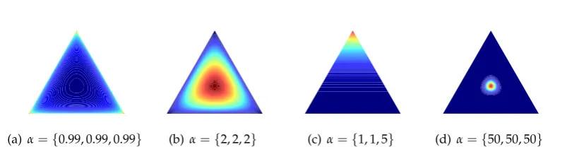
The Dirichlet distribution Dir(α) is defined over a finite simplex parameterized by a variable α = {α1, . . . ,αm}. This parameter specifies the concentration of samples in the simplex. Each point in this simplex can be thought of as a probability mass function (pmf) and consequently the joint is weighted sum of these pmfs (by α).
In Figure 2.6, we show examples of Dirichlet distribution with various values of parameter α. One important property of the Dirichlet distribution that is used in
building the Dirichlet process isaggregation. That is, if partitions of the sample space are joined, the resulting sample space is again a Dirichlet distribution where the values ofαs for that partition are aggregated.
Dirichlet process is an extension of the mixture model introduced earlier (refer to [39] for a complete introduction). It models the distribution over an infinite sample set as an infinite mixture of weighted Dirac delta functions. This infinite mixture becomes the Dirichlet distribution again when we employ the aggregation property on all the sample space regions. The parameterα(A)is the function of the region A
of this Dirichlet distribution and is the integral of all the point masses in the region, i.e. α(A) = R IA[x]dα(x) where IAis the indicator function of region Afor x in the
input space. For Dirichlet process, there is an additional parameter G that specifies the base distribution where the samples are generated from. Base distribution is the expected value of the Dirichlet process. It should be noted that while G can be either continuous or discrete, the Dirichlet process is always discrete. Similar to the Gaussian process where the marginals were Gaussian, in Dirichlet process the marginals are Dirichlet.
§2.2 Bayesian Modeling and Learning 21
A1
A2
A4
A3 A5
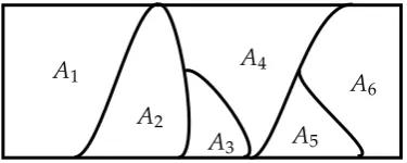
[image:37.595.225.413.115.190.2]A6
Figure 2.7: An illustration of the Dirichlet distribution and the partitioning of the space.
some probability one partition might break into two. As such, one way to construct the Dirichlet process is to consider the partitioning of the input space A={A1,A2}.
Then the distribution in Ais a Beta(α(A1),α(A2))with its expectation defined as α(A1)
α(A1) +α(A2)
= α(A1)
M .
Here, the denominator M denotes the mass of the region on which the probabil-ity is defined. When increasing the number of partitions, the joint distribution becomes Dirichlet with similar property. In particular for finite partitions A =
{A1,A2, . . . ,Am}the posterior p(A1), . . . ,p(Am)on given inputs{x1,x2, . . . ,xn}is Dir(α(A1) +n1, . . . ,α(Am) +nm)
where
ni = n
∑
j=1I[xj ∈ Ai],
the count for observations in partitionAi. The expectation of the posterior is [39]: E[x1,x2, . . . ,xn] =
M
M+nG(A) + n M+np˜
where ˜p is the empirical distribution, i.e., the distribution of observed points. This equation simply states on expectation a sample is drawn from the base distributionG
with a value proportionate to the mass (that is in the heart of sampling for the Dirich-let processes). Similarly, with a value proportionate to the number of observations it is assigned to one of the current partitions. Since this distribution is exchangeable, we have the following conditional:
p(xn+1 ∈ Am|x1,x2, . . . ,xn) =
M
M+nG(Am) + nm
M+np˜.
Again, probability of assigning a point xn+1 to a partition is proportionate to the
instance to be assigned to a more populous partition. Schemes such as Polya urn method, Chinese restaurant process and stick-breaking are developed around this central concept to provide various views for construction of the Dirichlet process [29, 39, 56, 67].
Another important property of the Dirichlet distribution is that it is a conjugate prior for the multinomial distribution. In other words, the simplex defined by the Dirichlet distribution is a distribution over parameter of the multinomial distribution. By integrating over all possible such parameters, we obtain a multinomial posterior. In the same way, one can use the Dirichlet distribution as a prior for the cluster probability p(ci =c)in Equation 2.5. We will see an example of using this property in Chapter 3.
2.3
Bayesian Inference
As mentioned before, Bayesian inference is the process of obtaining the posterior from the prior by incorporating the likelihood of the observations. In many practi-cal cases the integral of the posterior is intractable and approximations are needed. Although for simple problems with small dimensions numerical integration (such as quadrature method) can be performed, in practice these methods are infeasible in high dimensions. Also, since the posterior is obtained from the product of all the likelihoods with the prior, it can be highly multimodal. In this section we will discuss key Bayesian inference methods in the literature which will be used throughout the subsequent chapters.
In general, approaches to inference can be either deterministic or stochastic. In deterministic methods, the true posterior is used to constrain the approximate distri-bution so that is easier to work with. For example in variational methods, the true posterior is used as an upper bound on a predefined family of distributions (such as exponential family). These methods generally enjoy fast inference, however, the effectiveness of the approximation highly depends on the divergence measure and the distribution family used [54]. The stochastic methods typically draw samples directly from the posterior e.g. Markov Chain Monte Carlo methods. These methods are generally slower and computationally more demanding, but can be arbitrarily accurate in estimating the moments of the posterior.
2.3.1 Laplace Method
The first approximate Bayesian inference method that we will consider is the Laplace approximation [12, 55]. Laplace’s method uses the Taylor expansion of the log of the posterior at pointθ∗ as
log(p(θ|D)) ≈ log(p(θ∗|D)) +g>(θ−θ∗) +1 2(θ−θ
§2.3 Bayesian Inference 23
where
g =
∂log(p(θ|D))
∂θ
θ=θ∗
H =
∂2log(p(θ|D))
∂θ∂θ>
θ=θ∗ .
This expansion already looks like the log of Gaussian distribution. If we useθ∗at the mode (obtained from the MAP estimate), theng=0 and we get
p(θ|D) ≈ N(θ∗,−H−1).
Simply put, we obtain the point estimate of the posterior using MAP inference and use this point to compute the covariance matrix. Then, Laplace’s method ap-proximates the posterior with a unimodal Gaussian distribution centered at a mode of that posterior. As such, it ignores the complex multimodal shape of the posterior. Although the curvature of the posterior is captured in the hessian matrix of the log of the posterior, in general the exact shape of the posterior is not preserved in its Laplace’s approximation.
2.3.2 Variational Inference
Variational methods [12, 45, 88, 90, 92] have received significant attention in recent years and use the calculus of variations to have a better global approximation. Un-like Laplace’s method that is rather simplistic, variational methods can work with a larger family of distributions. Similar to Laplace’s method, variational methods involve finding a lower bound to the true posterior. Maximizing this lower bound can be done efficiently using well-established optimization algorithms. Therefore variational methods are efficient inference algorithms.
Since the difficult part of the inference is computing the normalizer, we use cal-culus of variation to rewrite it as
Z =
Z
p(D|θ)p(θ)dθ=
Z
p(D|θ)p(θ)
q(θ|ψ)
q(θ|ψ)dθ
where ψ is the collection of parameters that define q. The alternative distribution q is used to approximate the true posterior. Using−log as a convex transformation of
Zand Jensen’s inequality, we have
log(Z) ≥ Z
log p(
D|θ)p(θ)
q(θ|ψ)
q(θ|ψ)dθ,
therefore,
Z ≥ exp
Z
log
p(D|θ)p(θ)
q(θ|ψ)
q(θ|ψ)dθ
Maximizing the right hand side of this equation will achieve a tight lower bound on the normalizer. The tightness of this bound depends on the choice of q. It is easy to see this bound is equal to the negative of the KL-divergence between the two distributions. Therefore, this maximization over parameters ψ is equivalent to minimizing the KL-divergence between the approximate and the true posterior, i.e.
KL(q||p) =
Z
log
q(θ|ψ)
p(D|θ)p(θ)
q(θ|ψ)dθ.
The idea is that computing this integral with respect to q and working with the log is simpler because q is potentially a distribution with respect to which this in-tegral becomes tractable. This minimization objective is also known as I-projection (information projection) since it seeks to estimate the regions of the posterior that have higher density.
Various assumptions and constraints on the approximate distribution leads to several extensions namely, mean-field, Bethe method and cavity method [31, 90, 92]. For example, mean-field methods assume the parameters of the true posterior are independent which leads to simplification of the minimization of the KL divergence.
2.3.3 Expectation Propagation (EP)
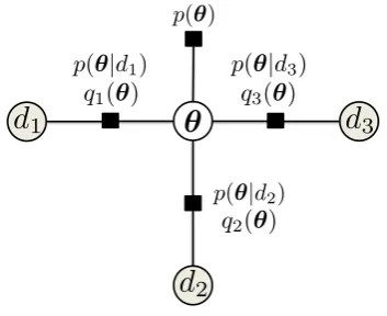
Another approximate Bayesian inference method isExpectation Propagation(EP) [55]. EP is an efficient algorithm for approximating factorized distributions. The gen-eral idea is that we can approximate the posterior by replacing each factor with an approximation and computing the product that permits a tractable posterior compu-tation. Iterating through this procedure for all factors will approximate the posterior. EP is presented in Algorithm 2.1 in detail. As is seen, first the approximate posterior
q(θ) is constructed from the prior and the initial estimate of each factor. Then iter-atively, each factor is replaced with its true likelihood (p(Di|θ)) and then updated accordingly for allnfactors. A graphical model of EP is shown in Figure 2.8.
Algorithm 2.1Expectation Propagation (EP)
q(θ) = p(θ)∏ni=1qi(θ)
whilenot convergeddo
fori=1,. . . ,ndo
compute cavity distributionq\i(θ) =q(θ)/qi(θ) compute tilted distribution ˜qi(θ) = p(Di|θ)qi(θ) setqnewi (θ) so that qnewi (θ)q\i(θ)≈q˜i(θ) updateq(θ) =qnewi q\i(θ)
end for end while
§2.3 Bayesian Inference 25
✓
d
2d
1d
3p(✓|d3)
p(✓|d1)
p(✓|d2)
q2(✓)
q1(✓) q3(✓)
[image:41.595.230.407.112.256.2]p(✓)
Figure 2.8: A graphical model for EP
distribution q\i(θ) by incorporating the given likelihood and the cavity distribution
p(Di|θ)q−i(θ). This draws further attention to the fact that using simple approxima-tion of each likelihood term (as probability of the condiapproxima-tionally independent variable
Di) and computing the approximate posterior from it is not a good approximation of the true posterior. Instead EP suggest using an approximation of each term that incorporates the approximations to other terms as well (i.e. effect of each observation individually on the posterior distribution). That is why the cavity distribution is re-quired to account for the other variables and their influence. If the approximation at each step is not required (computing tilted distribution is tractable), with this mes-sage passing view one can obtain the popular loopy Belief propagation algorithm [95] as a special case of EP.
The projection in this procedure is equal to minimizing the KL-divergence be-tween the true posterior and its approximation, i.e.
KL(p||q) =
Z
log
p(θ|D)
q(θ)
p(θ|D)dθ.
In particular, in the algorithm when the approximation of each factor is updated in
qnew
i (θ)q−i(θ)≈ q\i(θ), we minimize the KL divergence between this approximation and the true posterior. Interestingly when the distribution of q is in exponential family, it is easy to see that this minimization is equal to matching the expectations under p and q. This is known asmoment matching (matching mean, variance, etc.). Hence unlike variational inference, in EP the mass of the posterior is more important to be correctly estimated. Furthermore, as opposed to variational methods EP is zero-avoiding, meaning that if there is a non-zero density region in the posterior it will be considered in the approximations [45].
2.3.4 Sampling and Markov Chain Monte Carlo (MCMC)
In this section, we discuss stochastic methods for estimating the posterior. The gen-eral idea in stochastic methods is to draw samples from the posterior to estimate any desired expectation. For simple distributions, if the cumulative density function (CDF) is known, the samples can be easily drawn from its inverse function. However, in general many distributions that we are interested in (i.e. the posterior) may not have a tractable CDF. For further reading on stochastic methods refer to [32, 57, 79]. We closely follow [57].
2.3.4.1 Monte Carlo Methods
Monte Carlo (MC) methods are stochastic methods for unbiased estimation of the integrals with respect to a distribution by sampling. In particular, let’s imagine we are estimating the expectation of the posterior parameter, i.e.
Ep[θ] =
Z
θp(θ|D)dθ.
This integral is then estimated by an unbiased value obtained from the average of the samples, i.e.
Ep[θ] ≈ 1
N
N
∑
j=1θi θi ∼ p(θ|D).
As the number of samples grow, this average approaches the true expectation. Unlike the previous approaches, MC methods can be arbitrarily accurate depending on the number of samples.
In simple problems with low dimensions, one can perform rejection sampling, that is, generate samples ofθfrom a region that is easy to sample from and contains the posterior (e.g. a hypercube), and with some probability proportionate to the posterior’s density accept each sample. In high dimensional problems though, it is computationally costly to perform such sampling and almost all generated samples are rejected.
The difficulty with this approach is that samples generally have to be generated from the prior and weighted by the likelihood (likelihood weighting). Since the priors are typically far from the desired posterior, this process becomes slow and inefficient. The alternative approach is to construct the sequence of samples from the posterior distribution. Markov Chain Monte Carlo(MCMC) methods search the space and generate the samples that are provably from the posterior when the number of samples grows. It is known as Markovian since each sample is drawn conditioned on the previous one which forms a chain. In this search, MCMC generates more samples from the regions with higher density.