arXiv:1706.07067v1 [math.OC] 21 Jun 2017
interior–proximal primal–dual methods
Tuomo Valkonen∗
2017-06-23
Abstract We study preconditioned proximal point methods for a class of saddle point problems, where the preconditioner decouples the overall proximal point method into an al-ternating primal–dual method. This is akin to the Chambolle–Pock method or the ADMM. In our work, we replace the squared distance in the dual step by a barrier function on a sym-metric cone, while using a standard (Euclidean) proximal step for the primal variable. We show that under non-degeneracy and simple linear constraints, such a hybrid primal–dual algorithm can achieve linear convergence on originally strongly convex problems involv-ing the second-order cone in their saddle point form. On general symmetric cones, we are only able to show anO(1/N)rate. These results are based on estimates of strong convexity of the barrier function, extended with a penalty to the boundary of the symmetric cone.
Due to arXiv’s inability to handle biblatex properly, and refusal to accept PDFs, references are broken in this file. Please get the correctly typeset version from http://tuomov.iki.fi/publications/.
1
introduction
Interior point methods exhibit fast convergence on several non-smooth non-strongly-convex problems, including linear problems with symmetric cone constraints [1, 2, 3,4]. The meth-ods have had less success on large-scale problems with more complex structure. In particular, problems in image processing, inverse problems, and data science, can often be written in the form
(P) min
x G(x)+F(Kx)
for convex, proper, lower semicontinuousGandF, and a bounded linear operatorK. Often, with
GandF involving norms and linear operators, (P) can be converted into linear optimisation on symmetric cones. This is even automated by the disciplined convex programming approach of CVX [5,6]. Nonetheless, the need to solve a very large scale and difficult Newton system on each step of the interior point method makes this approach seldom practical for real-world problems. Therefore, first-order splitting methods such as forward–backward splitting, ADMM (alternating directions method of multipliers) and their variants [7,8,9, 10] dominate these application areas. In our present work, we are curiouswhether these two approaches—interior point and splitting methods—can be combined into an effective algorithm?
The saddle point form of (P) is
(S) min
x maxy G(x)+hKx,yi −F
∗(y).
A popular algorithm for solving this problem is the primal–dual method of Chambolle and Pock [10]. As discovered in [11], the method can most concisely be written as apreconditioned proximal point method, solving on each iteration forui+1
=(xi+1,yi+1)the variational inclusion
(PP0) 0∈H(ui+1)+Mi+1(u
i+1−ui),
where the monotone operator
H(u):=
∂G(x)+K∗y ∂F∗(y) −Kx
encodes the optimality condition0∈H(bu)for (S). For the standard proximal point method [12], one would takeMi+1 = I the identity. With this choice, the system (PP0) is generally difficult
to solve. In the Chambolle–Pock method thepreconditioningor step length operator is given for suitably chosen step length parametersτi,σi+1,θi > 0by
Mi+1 :=
τi−1I −K∗ −θiK σi−+11I
.
This choice ofMi+1decouples the primalxand dualyupdates, making the solution of (PP0)
fea-sible in a wide range of problems. IfGis strongly convex, the step length parametersτi,σi+1,θi can be chosen to yieldO(1/N2)convergence rates of an ergodic duality gap and the squared distancekxi−xbk2. If bothGandF∗are strongly convex, then the method converges linearly.
In our earlier work [13,14,15], we have modifiedMi+1 as well as the condition (PP0) to still allow a level of mixed-rate acceleration whenGis strongly convex only on spaces or sub-blocks of the variablex = (x1, . . . ,xm), and derived a corresponding doubly-stochastic
block-coordinate descent method. As an extension of that work, our specific question now is:
IfF∗encodes the constraintAy =bandy ∈ K
for a symmetric coneK,can we replaceMi+1in(PP0)by a non-linear interior point preconditioner
that yields tractable sub-problems and a fast, convergent algorithm?
Generalised proximal point methods motivated by interior point methods have been consid-ered before in [16, 17,18,19]. Here the approach has essentially been to replace the squared distance in the proximal point methodxi+1 :
=arg minx∈KG(x)+ 21τkx−xik2forminx∈KG(x)
by a suitable Bregman distance supported onintK ×intK, typicallyD(x,x′):=tr(x◦lnx−x◦
lnx′+x′−x). To the best of our knowledge, no convergence rates have been obtained using this approach. InSection 4of the present work, we will instead replace the squared distance in the proximal point step for the dual variabley by a more conventional barrier-based pre-conditioner−∇log det(y). With this, we are able to obtain convergence rates: in the general case onlyO(1/N), but linear convergence in the second-order cone under non-degeneracy and
A = ha,·ifora ∈ intK. We demonstrate these theoretical results by numerical experiments
The overall idea, how the theory works, is that the barrier-based preconditioner is strongly monotone on bounded subsets ofintK, and “compatible” with∂F∗on∂Kin such a way that these strong monotonicity estimates can, with some penalty term, be extended up to the bound-ary. This introduces some of the strong monotonicity that∂F∗itself is missing.
An interesting question for future research is, whether the results for general cones can be improved, or whether the second-order cone is special? Nevertheless, our present theoretical results makeprogress towards closing the gap between direct methods for (P), and primal–dual methods for (S): among others, forward–backward splitting for (P) is known to obtain linear convergence with strong convexity assumptions onG alone [20], but primal–dual methods generally still require the strong convexity ofF∗as well. For ADMM additional local estimates exist under quadratic [21,22] or polyhedrality assumptions [23]. On the other hand, it has been recently established that forward–backward splitting converges at least locally linearly even under less restrictive assumptions than the strong convexity ofG[24,25].
Our theoretical results depend on the convergence theory for non-linearly preconditioned proximal point methods from [14]. We quote the relevant aspects inSection 3. To use this theory, we need to compute estimates on the strong convexity of the barrier, with a penalty up to the boundary. This is the content of the latter half ofSection 2, after introduction of the basic Jordan-algebraic machinery for interior point methods on symmetric cones.
2 notation, concepts, and results on symmetric cones
We writeL(X;Y)for space of bounded linear operators between Hilbert spacesX andY. For anyA∈ L(X;Y)we writeN(A) for the null-space, andR(A)for the range. Also for possibly non-self-adjointT ∈ L(X;X), we introduce the inner product and norm-like notations
(2.1) hx,ziT := hT x,zi, and kxkT :=
p
hx,xiT, (x,z ∈X).
WithR := [−∞,∞], we write C(X)for the space of convex, proper, lower semicontinuous functions fromX toR. WithK ∈ L(X;Y),G ∈ C(X)andF∗∈ C(Y)on Hilbert spacesX andY, we then wish to solve the minimax problem (S) assuming the existence of a solutionbu=(bx,by) satisfying the optimality conditions0∈H(by), in other words
(OC) −K∗by ∈∂G(bx), and Kbx ∈∂F∗(by).
For a functionG, as above,∂G stands the convex subdifferential [26]. For a setC,∂C is the boundary. We denote byNC(x)= ∂δC(x)the normal cone to any convex setCatx ∈C, where δC is the indicator function of the setCin the sense of convex analysis.
InSection 4, we concentrate onF∗of the general form (2.2) in the next example.
Example 2.1 (From ball constraints to second-order cones). Very often in (P), we haveF(z)=
Ín
i=1αikzik2, where the norm is the Euclidean norm on Rm andz = (z1, . . . ,zn) ∈ Rmn.
ThenF∗(ys) = δB(0,αi)(ysi) forys = (y1s, . . . ,ysn) ∈ R
mn. We may lift each
s
yi =(yi,0,ysi), and replaceF ∗by
(2.2) Fˆ∗(y):=
n
Õ
i=1
δCi(yi), where Ci :={yi ∈ K |Ay =b},
where, the linear constraint is defined byAy := (y1,0, . . . ,yn,0)andb := (α1, . . . ,αn). The cone constraint is given byK =Ksocn for thesecond-order cone
Ksoc:={y =(y0,ys) ∈R1+m |y0 ≥ kysk}.
In the following, we look at the Jordan-algebraic approach to analysis on the second-order cone and othersymmetric cones.
2.1 euclidean jordan algebras
We now introduce the minimum amount of the theory of Jordan algebras necessary for our work. For further details, we refer to [27,28].
Technically, a realJordan algebraJ is a real (additive) vector space together with a bilinear and commutative multiplication operator◦ : J × J → J that satisfies the associativity conditionx ◦ (x2 ◦y) = x2◦ (x ◦y). Here we definex2 := x ◦x. The Jordan algebra J is
Euclidean(orformally real) ifx2+y2=0impliesx =y =0. We always assume that our Jordan algebras are Euclidean.
We will not directly need the last two technical definitions, but do rely on the very important consequence thatJhas a multiplicative unit elemente:x◦e=x for allx ∈ J. An elementx
ofJ is then called invertible, if there exists an elementx−1, such thatx◦x−1 =x−1◦x =e.
Example 2.2 (The Jordan algebra of symmetric matrices). To understand these and the
fol-lowing properties, it is helpful to think of the set of symmetricm×mmatrices. They form a Jordan algebra endowed with the productA◦B := 21(AB+BA). The inverse is the usual matrix inverse, as is the multiplicative identity. So are the properties discussed next.
An elementcin a Jordan algebraJ is anidempotent ifc◦c=c. It isprimitive, if it is not the sum of other idempotents. AJordan frame is a set of primitive idempotents{ei}ir=1 such that ei ◦ej = 0fori , j, andÍrj=1ej = e. The numberr is therankof J. For eachx ∈ J, there indeed exist unique real numbers{λi}ri=1, and a Jordan frame{ei}ir=1, satisfyingx =
Ír j=1λiei.
The numbersλi(x) = λi are called theeigenvalues ofx. If all the eigenvalues are positive, we
writex > 0and callx positive definite. Likewise we writex ≥ 0if the eigenvalues are non-negative, and callxpositive semi-definite. With the eigenvalues, we can define
(i) Powersxα :=Írj=1λαiei when meaningful,
(ii) The determinantdetx :=Îjλj, and
(iii) The tracetrx :=Írj=1λj.
(iv) The inner producthx,yi:=tr(x◦y), and the (v) Frobenius normkxk:= kxkF :=qÍrj=1λ2j =
p
The inner product is positive-definite and associative, satisfyinghx◦y,zi=hy,x◦zi. We also frequently write
λmax(x):= max i=1, . . .,r
λi(x) and λmin(x):= min
i=1, . . .,r
λi(x).
For conciseness, we define forx ∈ J the operatorL(x) byL(x)y := x ◦y. Thequadratic
presentation ofx—this is one of the most crucial concepts for us, as we will soon see when covering symmetric cones—is then defined asQx := 2L(x)2−L(x2). The invertibility ofx is
equivalent to the invertibility ofQx. Other important properties include [27,1]
(vi) Qαx =Qxα forα ∈R,
(vii) QQxy =QxQyQx (thefundamental formulaof quadratic presentations),
(viii) Qxx−1 =x, (ix) Qxe =x2, and
(x) det(Qxy)=det(x2)y =det(x)2y.
Moreover,Qxis self-adjoint with respect to the inner product defined above, and the eigenvalues
are productsλi(x)λj(x)[28,27], so that
(2.3) λ2min(x)kyk2≤ hQxy,yi ≤λmax(x)2kyk2 for all y when x ≥0.
Example 2.3 (The Euclidean Jordan algebra of quadratic forms). LetE1+m denote the space
of vectorsx =(x0,xs) ∈R1+mwithx0scalar. Setting
x◦y =(xTy,x0ys+y0xs),
we make(E1+m,◦)into a Euclidean Jordan algebra. The identity element ise = (1,0), rank r =2, and the inner product is
(2.4) hx,yi=2xTy.
Defining the diagonal mirroring operatorR:= 01 0−I
, we find thatdetx =xTRx =x02−kxsk2,
andx−1 =Rx/detxwhendetx ,0.
2.2 symmetric cones
Thecone of squares of a Euclidean Jordan algebraJ is defined as
K :={x2 |x ∈ J }.
The cones generated this way are precisely the so-called symmetric cones [27]K∗ = −K, or the self-scaled cones of [4]. Their important properties include [27,28]:
(i) intK ={x ∈ J |x is positive-definite}= {x ∈ J |L(x)pos. def.}. (ii) hx,yi ≥0for ally ∈ Kiffx ∈ K, and
(iii) hx,yi> 0for ally ∈ K \ {0}iffx ∈intK. (iv) Qx forx ∈intK mapsKonto itself.
(vi) For anyx,y ∈ K,hx,yi=0iffx◦y =0[29].
For application to interior point methods, and in particular for our work, the following proper-ties are particularly important:
(vii) The barrier functionB(x):=−log(detx)tends to infinity asx goes tobdK. (viii) ∇B(x)=−x−1and∇2B(x)=Q−x1(differentiated wrt. the norm inJ).
(ix) The normal coneNK(x)=−{y ∈ K | hy,xi=0}forx ∈ K[30, Lemma 3.1].
Example 2.4 (The cone of symmetric positive definite matrices). In the Jordan algebra of
symmetric matrices fromExample 2.2, the cone of squares is the set of positive semi-definite symmetric matrices.
Example 2.5 (The second order cone). The cone of squares of the Jordan algebraE1+m of
quadratic forms is the second order cone that we have already seen inExample 2.1,
K =Ksoc:={x ∈E1+m |x0 ≥ kxsk}.
If0,x ∈bdK, we havex2 = 2x0x. Rescaled, we get a primitive idempotentc = x/√2x0.
The only primitive idempotent orthogonal tocisc′=Rx/√2x0. Therefore, the normal cone
NK(x)={−αRx |α ≥ 0}.
One has to be careful with the fact that the expressions for the barrier gradient and Hes-sian in(viii)are based on the inner product (2.4) inE1+m. This is scaled by the factorr =2
with respect to the standard inner product onR1+m.
2.3 linear optimisation on symmetric cones
LetA ∈ L(J;Rk) for an arbitrary Euclidean Jordan algebraJ with the corresponding cone of squaresK. We will frequently make use of solutions(yµ,dµ,zµ) ∈intK ×intK ×Rk to the
system
(SCLPµ) Ay =b, A∗z+c =d, y◦d =µe, y,d ∈intK.
These are meant to approximate solutions(by,db,bz) ∈ K × K ×Rk to the system
(SCLP) Ay =b, A∗z+c =d, y◦d =0, y,d ∈ K.
The system (SCLP) arises from primal–dual optimality conditions for linear optimisation on symmetric cones, specifically the problem
min y∈K,Ay=b
hc,yi.
The system (SCLPµ) arises from the introduction of the barrier in the problem
(2.5) min
y∈K,Ay=b
The set of solutions to (SCLPµ) for varyingµ >0is called thecentral path. From [2, Theorem
2.2] we know that if there exists a primal–dualinterior feasible point, i.e., some(y∗,d∗,z∗) ∈ intK ×intK ×Rksuch thatAy∗=bandA∗z∗+c =d∗, then there exists a solution(yµ,dµ,zµ)
to (SCLPµ) for everyµ > 0. In particular, if there exists a solution for someµ >0, there exist a
solution for allµ >0. In fact, we have the following:
Lemma 2.1. Suppose there exists a primal interior feasible pointy∗∈intK ∩ {y ∈ K |Ay =b}.
Then there exists a solution(yµ,dµ,zµ) ∈intK ×intK ×Rk to(SCLPµ)for allµ > 0.
Proof. The article [2] considers a more general class of linear monotone complementarity prob-lems (LMCPs) than our our SCLPs (symmetric cone linear programs). For the special case of SCLPs, our assumption on the existence ofy∗implies that the feasible set in (2.5) non-empty and closed. Since the objective function level-bounded, proper, and lower semicontinuous, the problem (2.5) has a solutiony. Thisyhas to satisfy (SCLPµ) for somedandz. Now [2, Theorem
2.2] applies.
Practical methods [4,1] for solving (SCLP) by closely following the central path are based on scaling the iterates(yi,di)byQpfor a suitablep ∈intK. We will need this scaling for different
purposes, and therefore recall the following basic properties.
Lemma 2.2. Letp ∈intK, andy,d ∈ K. Defineey :=Q1p/2y, andd
e:=Q −1/2 p d. Then
(i) y◦d =0if and only ifey◦d e=0.
(ii) Ify,d ∈intK andµ >0, theny◦d =µe if and only ifey◦d e=µe.
(iii) (SCLP)(resp.(SCLPµ)) is satisfied fory andd if and only if it is satisfied forey andd
ewith
Aandcreplaced byAe:=AQ−p1/2andc
e:=Q −1/2 p c.
Proof. The claim(i)is a consequence of the propertiesSection 2.2(iv)and(vi). The claim(iii)is the content of [1, Lemma 28]. Finally, to establish(iii), the remaining linear equations in (SCLP)
and (SCLPµ) are obvious.
As a last preparatory step, before starting to derive new results, we say that solutionsy,d ∈ K
to (SCLP) arestrictly complementary ify ◦d = 0andy +d ∈ intK. We say thaty isprimal
non-degenerateif
(2.6) v =A∗zandy◦v=0 =⇒ v =0.
Likewised isdual non-degenerate if
(2.7) Av =0andd◦v=0 =⇒ v =0.
2.4 convergence rate of the central path
We now study convergence rates for the central path, which we will need to develop approxi-mate strong monotonicity estiapproxi-mates. Some existing work can be found in [31], but overall the results in the literature are limited; more work can be found on the properties and mere exis-tence of limits of the central path [32,33,34,35,36]. After all, in typical interior point methods, one is not interested in solving (SCLPµ) exactly; rather, one is interested in staying close to the
Lemma 2.3. Letby,db∈ K andbz ∈ Rk solve(SCLP). Also lety
µ,dµ ∈ intK andzµ ∈ Rk solve
(SCLPµ)for someµ > 0. Ifby anddbare strictly complementary, and both primal and dual
non-degenerate, then
(2.8) kyµ−byk ≤
2µ√r λmin(M
b
y,db)
,
where λmin(My,d) > 0is the minimal eigenvalue of the the linear operatorMy,d ∈ L(J;J )
defined aty,d ∈ J forη∈ N(A)andξ ∈ R(A∗)by
My,d(ξ +η):=L(y)ξ +L(d)η.
Proof. Observe that(yµ,dµ,zµ)solves (SCLPµ) if and only ifyµ =by+∆yanddµ =db+∆dwith
∆y ∈ N(A), ∆d ∈ R(A∗), and Mby
,db(
∆y+∆d)=µe−∆y◦∆d.
Here we have used the fact thatby◦db=0. We may rearrange the final condition as
1 2Mby,db(
∆y+∆d)=µe− 1
2(yb+∆y) ◦∆d− 1
2∆y◦ (db+∆d).
This simply says that
1 2
M
b
y,db+
Myµ,dµ
(∆y+∆d)=µe.
From [2, Corollary 4.9] we know that the operatorMyb
,db
is invertible when the solution(by,db)
is strictly complementary and both primal and dual non-degenerate. Moreover, for (yµ,dµ)
satisfying (SCLPµ), we know from [2, Corollary 4.6] thatMyµ,dµ is invertible. In fact, both
Myµ,dµ and Myb ,db
are positive definite: in both cases,(y,d) = (yb,db), and(y,d) = (yµ,dµ),
the mapm(ζ) := hζ,My,dζi is continuous on J, while m(η) > 0 andm(ξ) > 0 for all
η ∈ N(A) andξ ∈ R(A∗). For (y,d) = (yb,db) the positivity follows from the assumed pri-mal and dual non-degeneracy, as the operatorsL(by) andL(db) are positive semi-definite. For
(y,d) = (yµ,dµ) ∈ intK × intK, the operatorsL(yµ) andL(dµ) are positive definite; see
Section 2.2(i). By an interpolation argument, a contradiction to invertibility would therefore
be reached ifMy,d were not positive semi-definite on the whole space [?, cf.]proof of Lemma 32]as-2003.
As a sum of invertible positive definite operators, it now follows thatM
b
y,db+
Myµ,dµ is in-vertible. Consequently we estimate
k∆yk ≤ k∆y+∆dk=2µkekk(M
b
y,db+
Myµ,dµ) −1
k
≤ 2µ
√ r λmin(Myb
,db+
Myµ,dµ)
≤ 2µ
√ r λmin(Mby
,db)
,
2.5 strong monotonicity of the barrier
If the barrierB(y) = −log(dety) is as in Section 2.2, then in the next lemmad = −∇B(y). Therefore, the lemma provides an estimate of strong monotonicity of the gradient of the barrier.
Lemma 2.4. Lety,y′∈intK, and denoted :=y−1, andd′ :
=(y′)−1. Then
(2.9) − hd′−d,y′−yi ≥ 1
λmax(y′)λmax(y)ky
′−yk2.
Proof. There exists a uniquew ∈intKs.t.d′=Qw−1yandd =Qw−1y′; see, e.g., [4, Corollary 3.1].
We thus see (2.9) to hold if
(2.10) Qw−1 ≥ 1
λmax(y′)λmax(y). In fact,w is given by the Nesterov–Todd direction
(2.11) w =
Qy−1/2(Qy1/2d′)1/2 −1
.
Indeed, using the fundamental formula for quadratic presentations (Section 2.1(vii)), we see
(2.12) Qw−1 =Qw−1 =QQ
y−1/2(Qy1/2d′)1/2 =Qy−1/2Q 1/2
Qy1/2d′Qy−1/2.
Following [37, p.42], from this we quickly compute
Qw−1y =Qy−1/2QQ1/2
y1/2d′
e =Qy−1/2Qy1/2d′=d′.
Invertingd′ = Qw−1y, we get(d′)−1 = y′ = (Qv−1y)−1 = Qvy−1 = Qvd. Henced = Qv−1y. This
establishes the claimed properties ofw. Continuing from (2.12), we also have
(2.13) Qw−1=Qy−1/2[Qy1/2Qd′Qy1/2]1/2Qy−1/2
FromSection 2.1(i)and (2.3), we observe thatQd′ =Qy−1′ ≥λmax(y′)−2I. Thus
(2.14) Qw−1 ≥ 1
λmax(y′)Qy−1/2[Qy]1/2Qy−1/2 =
1
λmax(y′)Qy−1/2 ≥
1
λmax(y′)λmax(y).
This proves (2.10) and consequently (2.9).
We now extend the estimate to the boundary ofKwith a penalty using the approximations
formSection 2.4.
Lemma 2.5. Lety,d ∈ intK andyb,db∈ K withd = y−1, andby ◦db= 0. Suppose there exist
y′,d′ ∈ Ksuch that
(2.15) hdb−d′,y−byi=0 and y′◦d′ =e.
Then for anyα ∈ (0,1)and anya ∈intK holds
(2.16) − hd−db,y−byi ≥ 1−α
λmax(ey)λmax(ye′)ky −byk
2 Qa−
λmax(d)λmax(d′) 4α ky
′−byk2,
Proof. LetQw be as in the proof ofLemma 2.4.
(2.17)
−hd−db,y−byi (2.15=) −hd−d′,y−byi =hy−y′,y−ybiQw−1
= hy−yb,y−byiQ−1
w +hby−y
′,y −byi
Q−1
w ≥ (1−α)ky −byk2
Q−1
w − 1
4αky′−bykQ2−1
w
.
In the final step we have used Cauchy’s inequality. Letw
e:=Qa1/2w. By the fundamental formula of quadratic presentations (Section 2.1(vii)),
Qw−1 =Qa1/2Q−1 Qa1/2wQ
1/2 a =Q
1/2 a Qw−1
e
Qa1/2.
We also observe using fundamental formula of quadratic presentations thatw
eisw from (2.11) computed with the transformed variablesey =Q1a/2y andd
e ′
=Qa−1/2d′. We therefore estimate
Q−1
e
w as in (2.14). Since (2.13) implies
Qw−1=Qd1/2[Qd−1/2Qd′Qd−1/2]1/2Qd1/2,
we also estimateQw−1 ≤λmax(d′)λmax(d). Thus (2.16) follows from (2.17).
Lemma 2.6. Lety,d ∈intKandby,db∈ Kwithu◦d =µefor someµ >0, andby◦db=0. Suppose
there existy′,d′∈ Ksuch thathdb−d′,y−byi=0andy′◦d′=µe. Then for anyα ∈ (0,1)holds
(2.18) − hd−db,y −byi ≥ (1−α)µ
λmax(ey)λmax(ye′)ky−y′k
2 Qa−
λmax(d)λmax(d′) 4α µ ky
′−byk2.
Proof. We applyLemma 2.5withdb,d, andd′replaced bydb/µ,d/µ, andd′/µ. This causes the right-hand-side of the estimate (2.16) to be multiplied byµ, along with bothλmax(d)andλmax(d′)
to be divided byµ.
Applied to solutions of (SCLPµ), we can estimateλmax(y)andλmax(y′).
Proposition 2.7. SupposeAy =bimplies ha,yi =b0for somea ∈ intK andb0 > 0. Fixµ > 0,
and let (y,d,z) ∈ intK ×intK ×Rk solve(SCLP
µ). Likewise, suppose(yµ,dµ,zµ) ∈ intK × intK ×Rk solves(SCLP
µ)forc=cˆ, where(by,db,bz)solves(SCLP)forc =cˆ. Ifbyanddbare strictly
complementary,dbdual non-degenerate, andbyprimal non-degenerate, then for anyα ∈ (0,1)holds
(2.19) − hd−db,y−byi ≥ (1−α)µ
b02 ky−byk 2 Qa−
Cc,µCcˆ,µr
αλmin(M
b
y,db)
2µ,
where for some fixedy∗ ∈intK withAy∗=bthe constants
(2.20) Cc,µ :=
µr+2b0kckQ−1
Proof. We begin by applying Lemma 2.6 with(y′,d′) set to the µ-approximation(yµ,dµ) to (by,db)provided byLemma 2.3. Inserting (2.8) into (2.18), we therefore obtain
(2.21) − hd−db,y−byi ≥ (1−α)µ λmax(ey)λmax(eyµ)k
y−yµkQ2a−
µλmax(d)λmax(dµ)r αλmin(Mby
,db)
2 .
It remains to estimate the eigenvalues in this expression.
First of all, we easily derive the necessary bounds onλmax(ey)andλmax(y′)as
(2.22) λmax(ey) ≤tr(ey)=he,eyi= ha,yi=b0.
Secondly, regarding the estimate on λmax(d), we fix somey∗ ∈ intK satisfyingAy∗ = b. Such a point exist by our assumption of there existing solutions to (SCLPµ); see alsoLemma 2.1.
Sinced=A∗z+c for somez ∈Rk, andd◦y =µe, we then derive
λmin(y∗)λmax(d) ≤λmin(y∗)he,di ≤ hy∗,di= hey∗,d ei = hye,d
ei+hye ∗−ey,d
ei=µr+hye ∗−ye,c
ei
≤ µr+kc
ek(λmax(ey)+λmax(ey ∗)) ≤ µr
+2b0kc
ek.
In the last inequality we have used (2.22) for bothyeandey∗. Sincey∗∈intK, so thatλmin(y∗) >0, andkc
ek= kckQa−1, this gives the claimed bounds onλmax(d)andλmax(d
′).
2.6 strong monotonicity of the barrier in the second-order cone
In the second-order cone K = Ksoc ⊂ E1+m, under suitable constraintsAy = b, we have a
stronger result.
Lemma 2.8. Supposey,y′,d,d′∈intKsocwithy◦d =y′◦d′=µe for givenµ >0. Then
(2.23) − hd−d′,y−y′iJ ≥ det(d)+det(d
′)
µ ky−y
′k2
−R,
whereky−y′k−2R :=kys−ys′kR2m− (y0−y0)′ 2=−det(y−y′).
Proof. We haved = µRy/det(y) = µ−1det(d)Ry. Likewised′ = µ−1det(d′)Ry′. We write for brevityβ:=µ−1det(d)andβ′:=µ−1det(d′). Then
−hd−d′,y−y′iJ =−hβRy−β′Ry′,y−y′iJ =2hβy−β′y′,y−y′i−R,
where the second “inner product” ishx,yi−R :=−hRx,yiR1+m. We can thus write
−hd−d′,y−y′iJ =2βky−y′k2−R +2(β−β′)hy′,y−y′i−R
as well as
−hd−d′,y −y′iJ =2β′ky−y′k−2R+2(β−β′)hy,y−y′i−R.
Summing these two expressions we deduce
(2.24) − hd−d′,y−y′iJ =(β+β′)ky−y′k−2R +(β−β′)(kyk 2
−R− ky′k 2
Now observe that
kyk−2R =y 2
0− kysk2=−det(y)=−µ2/det(d).
Thus
(β−β′)(kyk−2R− ky′k−2R)=µ(det(d) −det(d′))(det(d′)−1−det(d)−1) =µ(det(d′) −det(d))2/(det(d)det(d′))>0.
This and (2.24) immediately prove the claim.
For solutions of (SCLPµ) with one-dimensional linear constraints, we can extend the estimate
to the boundary with some penalty. For this, we first bound the determinant with the distance
DF(w,d):= kQw1/2d−µw,dek for µw,d = hw,di/r, (w,d ∈ K).
This distance is typically used to define the so-called short-step neighbourhood of the central path [?, see, e.g.,]]as-2003.
Lemma 2.9. Supposey,d ∈ intKsoc withy ◦d = µe and ha,yi = b0 for someµ,b0 > 0 and
a ∈intKsoc. Then
(2.25) 2µ
2
+√2b0DF(a−1,d)µ
b20det(a) ≤det(d) ≤
4µ2+√2b0DF(a−1,d)µ b02det(a) .
Proof. We defineey := Q1a/2y, andd
e := Q −1/2
a d. Then he,yei = ha,yi = b0, and by [1, Lemma
28],ey ◦d
e= µe. These conditions expand toy0dee0+eys
T
s
d
e= µ,ey0eds+de0eys= 0, and2ey0 =b0. (In the latter, recall that theE1+m-inner product satisfieshe,eyi =2eTey.) We reduce this system to
d
e
2 0− kds
ek
2 −2d
e0µ/b0=0, from where we solve
(2.26) d
e0 =
µ + q
µ2
+b02kds
ek
2
b0
.
Thus
det(d
e)=de
2 0− kds
ek
2
=
2µ2+2µ q
µ2
+b02kds
ek
2
b02 ,
from which we easily estimate
(2.27) 2µ
2
+2µb0kds ek
b20 ≤det(de) ≤
4µ2+2µb0kds ek
b02 .
To finish deriving (2.25), from Section 2.1(x)we recall thatdet(d
e) = det(a)det(d). We also haverd
e0= hde,ei= hd,a −1
ifor the rankr =2, so
(2.28) √2kds
ekRn = kde−de0ekJ = kQ −1/2 a d−µa−1
,dekJ =DF(a −1,d
),
where we emphasise the standard Euclidean norm onds
e∈ R
n versus the√2-scaled standard
IfDF(a−1,db) > 0, or alternativelydet(by) > 0, then the next proposition shows local strong
monotonicity of the barrier ford close todbandµ > 0small. Moreover, ifDF(a−1,db) > 0, the
factor of strong monotonicity does not vanish asµ ց0.
Proposition 2.10. LetK = Ksoc, and supposeAy =bimplies ha,yi=b0for somea ∈intK and
b0 >0. Let(y,d,z) ∈intK ×intK ×Rk solve(SCLP
µ), and likewise that(by,db,bz) ∈ K × K ×Rk
solve(SCLP)forc =bc. Then
(2.29) − hd−db,y−ybi ≥ µ+2
−1/2b
0[DF(a−1,d)+DF(a−1,db)]
b02 ky−byk 2 Qa−µ
+ 2 −1/2b
0DF(a−1,db)µ 2µ+2−1/2b0DF(a−1,d)
+ µ+2 −1/2b
0DF(a−1,d) b02/2 det(Q
1/2 a yb).
Proof. We have
(2.30) 0=by◦db=(by0db0+bys Tb
s
d,yb0bds+db0bys).
Sinceha,byi =b0 > 0, andyb∈ K, necessarilyby0 > 0. Since, moreover,yb, 0, we cannot have
b
d ∈ intK foryb◦db= 0to hold. Therefore0 = det(db) =db20− kbdsk2. It follows from (2.30) that
b
d =βRb by for
(2.31) βb=−bys
Tb s d b y2 0
= db0 b
y0 = kbdskRm
b
y0 = √
2DF(a−1,db) b0 ≥
0.
In the final step we have reasoned as in (2.28). We may therefore repeat the steps ofLemma 2.8
until (2.24) to obtain
(2.32) − hd−db,y −byi=(β+βb)ky−byk−2R+(β−βb)(kyk−2R− kbyk−2R).
We havedet(by) = −kbyk−2R = by02− kbysk2 ≥ 0. If this is non-zero,by ∈ intK. But in that case
b
y ◦db=0impliesdb=0, and consequentlyβb=0. Thusβbkbyk−2R = 0whether or notkbyk−2R =0.
Usingkyk2−R =−det(y)= −µ2/det(d)andβ=det(d)/µ, we therefore obtain from (2.32) that
(2.33) − hd−db,y−byi =(µ−1det(d)+βb)ky−byk−2R −µ+
b
β µ2 det(d) +
det(d)det(by) µ .
Ifa =e, we havey0 = by0 = b0/2, so that2ky −byk2−R = ky −byk 2
J. The final equality from (2.31) also givesβb=√2DF(e,db)/b0. With the help ofLemma 2.9, (2.33) thus yields
−hd−db,y−byi ≥ 2µ+ √
2b0[DF(e,d)+DF(e,db)]
b20 ky−byk 2
−µ
+
√
2b0DF(e,db)µ
4µ+√2b0DF(e,d)
+ 2µ +
√
2b0DF(e,d) b2
0
det(by). (2.34)
Ifa ,e, we defineye:=Q1a/2y, andd
e:=Q −1/2
a d as inLemma 2.9. Then(ey,d
e,z)continues to satisfy (SCLPµ) withAreplaced byAe:= AQa−1/2andc
e:=Q −1/2
a c. The same holds with (SCLP)
foreby := Q1a/2by anddb
e:=Q −1/2
a db. Therefore, (2.34) holds for these transformed variables. Since DF(e,d
e)=DF(a
−1,d), as well askey−ebyk2
= ky−bykQ2a, and−hd−d
′,y−y′i =−hd
e−edb,ey−ebyi,
we obtain the claim.
Corollary 2.11. LetK = Ksoc, and supposeA = ha, ·i for somea ∈ intK. Suppose moreover
that ha−1,ci = ha−1,bci = 0. Let(y,d,z) ∈ intK ×intK ×Rk solve(SCLPµ), and likewise that (by,db,bz) ∈ K × K ×Rk solve(SCLP)forc =bc. Ifbc ,0, then
−hd−db,y−byi ≥ µ +2
−1/2b
0[kckQ−1
a +kbckQ−a1]
b02 ky−ybk 2 Qa−µ.
(2.35)
Otherwise, ifbc =0withby =ba−1/2, then
(2.36) − hd−db,y−ybi ≥ µ+2
−1/2b 0kckQa−1
b02 ky−byk 2 Qa.
We say that (2.35) is strong monotonicity of the barrier “with a penalty”,µ.
Proof. We do not until the very end of the proof use the assumptionA= ha, ·i. For now, we use the weaker assumption thatAy = bimpliesha,yi = b0. We applyProposition 2.10. This gives
(2.37) − hd−db,y−byi ≥ µ +2
−1/2b0
[DF(a−1,d)+DF(a−1,db)]
b02 ky−ybk 2 Qa−µ
+ 2 −1/2b0D
F(a−1,db)µ 2µ+2−1/2b0DF(a−1,d)
+ µ+2 −1/2b0D
F(a−1,d) b02/2 det(Q
1/2 a yb).
IfDF(a−1,db)=0, by assumptionby =2b0a−1. This impliesdet(Qa1/2by)=b0/2. Consequently
µ+2−1/2b0DF(a−1,d) b02 det(Q
1/2 a by) ≥
µ 2.
Therefore no penalty is imposed, and (2.37) reduces to
(2.38) − hd−db,y−byi ≥ µ+2
−1/2b
0DF(a−1,d)
b02 ky−byk 2 Qa.
Suppose then thatDF(a−1,db) > 0. On the right hand side of (2.37), only the term −µ is
negative. Thus the condition holds if
(2.39) − hd−db,y−byi ≥ µ+2
−1/2b0
[DF(a−1,d)+DF(a−1,db)]
Finally, using our assumptions thatA = ha, ·i andha−1,ci = 0, we haved = za +c and
µa−1,d = ha −1,di/r
=zfor somez ∈R. Thus
(2.40) DF(a−1,d)= kQa−1/2(d−za)k = kckQa−1.
Likewise DF(a−1,db) = kbckQ−1
a . Therefore, the cases DF(a
−1,db
) > 0 andDF(a−1,db) = 0 are equivalent to the cases on kbck in the statement of the corollary. Inserting (2.40) into (2.38)
consequently yields the claimed estimates.
3 an abstract preconditioned proximal point iteration
In this section, we recall some of the core results from [14]. We start by setting
(3.1) H(u):=
∂G(x)+K∗y ∂F∗(y) −Kx
,
and for someτi,ϕi,σi+1,ψi+1 >0, defining the step length and “testing” operators
(3.2) Wi+1:=
τiI 0 0 σi+1I
, and Zi+1 :=
ϕiI 0 0 ψi+1I
.
We also letVi+1 : X ×Y ⇒ X ×Y for eachi ∈ N be an abstract non-linear preconditioner, dependent on the current iterateui. Then we consider the generalised proximal point method, which involves solving
(PP) 0∈Wi+1H(ui+1)+Vi+1(ui+
1 )
for the unknown next iterateui+1. To obtain convergence rates for the resulting method, the
idea from [14,13] will be to analyse the inclusion obtained after multiplying (PP) by the testing operatorZi+1.
AssumingG to be (strongly) convex with factorγ >0, we also introduce
Ξi
+1(γ):=
2γτiI 2τiK∗ −2σi+1K 0
,
which is an operator measure of strong monotonicity ofH.
The next lemma, which is relatively trivial to prove [14], forms the basis from which our work proceeds.
Theorem 3.1. Let us be givenK ∈ L(X;Y),G ∈ C(X), andF∗∈ C(Y)on Hilbert spacesX andY.
For eachi ∈N, for someVi′
+1 :X ×Y ⇒X ×Y andMi+1 ∈ L(X ×Y;X ×Y), take (3.3) Vi+1(u):=Vi′+1(u)+Mi+1(u−u
Assume that(PP)is solvable,Zi+1Mi+1is self-adjoint, andGis (strongly) convex with factorγ ≥0.
If for alli ∈Nthe estimate
(C0-Γ) 1 2ku
i+1−uik2
Zi+1Mi+1 | {z }
step length in local metric
+ 1
2ku
i+1−buk2
Zi+1(Ξi+1(γ)+Mi+1)−Zi+2Mi+2 | {z }
linear preconditioner update discrepancy
+h∂F∗(yi+1) −∂F∗(yb),yi+1−ybiΨi+1Σi+1 | {z }
variably useful remainder fromH
+hZi+1Vi′+1(u
i+1 ),ui+1
−bui
| {z }
from non-linear preconditioner
≥ −∆i
+1
holds, then
(3.4) 1
2ku N
−bukZ2
N+1MN+1 ≤
1 2ku
0
−bukZ21M1 +
NÕ−1
i=0
∆i
+1, (N ≥ 1).
Proof. This is [14, Theorem 3.1] specialised to scalar step length and testing operatorsTi =τiI,
Φi =ϕiI,Σi+1=σi+1I, andΨi+1 =ψi+1I, as well aseΓ=γ I.
It is possible to extend this theorem to provide an estimate on an ergodic duality gap [?, see]Theorem 4.6]tuomov-proxtest. For the sake of conciseness, we have however decided against including such estimates in the present work. For this reason, in the following, we concentrate on strongly convexG.
4 a primal–dual method with a barrier preconditioner
LetF(y):=δ{A·=b}(y)+δK(y)for someA∈ L(J;Z), whereJ andZ are Hilbert spaces,J also a Euclidean Jordan algebra. LetK be the cone of squares ofJ. We suppose there exists somey ∈ intKwithAy =b. Then the subdifferential sum formula (see, e.g., [26]) applies, so that
(4.1) ∂F∗(y)= (
{A∗z |z ∈Z}+NK(y), Ay =bandy ∈ K,
∅, otherwise.
In particular, ify ∈intK withAy =b, then∂F(y)= {A∗z |z ∈Z}. Note fromSection 2.2(ix) and(vi)that
NK(y)={−d |d ∈ K, hp,di=0} (y ∈ K).
Thus0∈H(bu)may also be written as the existence of(bx,by,db,bz) ∈X × K × K ×Z with
(IOC) −K∗by ∈∂G(bx), Aby =b, A∗bz−Kbx =db, by◦db=0.
4.1 a general estimate for dual barrier preconditioning
To construct algorithms with the help of the theory from Section 3, we have to construct the preconditionerVi+1(ui+1):=Vi′+1(ui+1)+Mi+1(ui+1−ui). We specifically take
(4.2) Mi+1=
I 0 0 0
, and Vi′+1(ui+1)
=(0,σi+1[K(xi+
1
−xi) −di+1]),
wheredi+1 ∈ intK is defined to satisfy yi+1 ◦di+1 = µ
i+1e for some µi+1 > 0. The term σi+1K(xi+1 −xi)inVi′+1 decouples the primal and dual updates so that(PP) may be written as
the system
0∈τi∂G(xi+1)+τiK∗yi+1+(xi+1−xi), (4.3a)
0∈σi+1[A∗zi+1−Kxi−di+1], as well as (4.3b)
yi+1◦di+1
= µi+1e and Ayi+1=b with yi+1,di+1 ∈intK.
(4.3c)
For this general setup, we have the following lemma:
Lemma 4.1. LetF∗have the structure(4.1). TakeMi+1andVi′+1according to(4.2). Suppose for some
ωi+1,δi+1 ∈Rfor alli ∈Nthat
−hdi+1−db,yi+1−byi ≥ω
i+1kyi+1−ybk2−δi+1,
(4.4a)
ψi+1σi+1=ϕiτi, (4.4b)
2ωi+1 ≥τikKk
2, and
(4.4c)
ϕi+1 ≤ϕi(1+2τieγ).
(4.4d)
Then(C0-Γ)holds with∆i
+1 =ψi+1σi+1δi+1, andZi+1Mi+1 is self-adjoint with
(4.5) Zi+1Mi+1 =
ϕiI 0 0 0
≥0.
Proof. The condition (C0-Γ) now reads
(4.6) 1
2ku i+1
−uikZ2 i+1Mi+1 | {z }
step in local norm
+ 1
2ku i+1
−bukD2 i+2 | {z }
lin. precond. upd. d.
+ψi+1σi+1hK(xi+1−xi),yi+1−ybi
| {z }
de-coupling term fromV′
+ψi+1σi+1hA∗(z
i+1
−bz),yi+1
−byi −ψi+1σi+1hd
i+1
−db,yi+1 −byi
| {z }
F∗term from (C0-Γ) as well asdi+1fromV′
≥ −∆i
+1
with the linear preconditioner update discrepancy
Di+2:=Zi+1(Ξi+1(γ)+Mi+1) −Zi+2Mi+2.
The expansion and estimate (4.5) are trivially verified along with the self-adjointness of
Zi+1Mi+1. This expansion allows us to write
Di+2=
ϕi(1+2τiγ)I−ϕi+1I 2ϕiτiK∗ −2ψi+1σi+1K 0
We use (4.4b) to cancel the off-diagonals ofDi+2in (4.6). Then we use the fact thatA(yi+1−by)=0 to cancel the first term on the second line of (4.6). Finally, we use∆i
+1 =ψi+1σi+1δi+1and (4.4a) to estimate the second term on the second line of (4.6). This gives the condition
(4.7) ϕi
2 kx i+1
−xik2+ψi+1σi+1ωi+1 2 ky
i+1
−byk2+ϕi(1+2γτi) −ϕi+1
2 kx
i+1 −xbk2
+ψi+1σi+1hK(x
i+1
−xi),yi+1
−byi ≥0.
Application of (4.4d), as well as Cauchy’s inequality to the inner product term, shows that (4.7) and consequently (C0-Γ) is satisfied if
ψi+1σi+1ωi+1 ≥
1 2ϕ
−1 i ψi2+1σ
2 i+1KK
∗.
This follows from (4.4b) and (4.4c).
We defineτi through (4.4c) for a lower boundω∗,i+1 ofωi+1. Likewise, we take (4.4d) as an equality as the definition ofϕi+1. We observe thatσi+1 andψi+1 are irrelevant to the algorithm in (4.3), as will be the specific choice ofϕ0 > 0to the satisfaction of (4.4). Takingϕ0 = 1, we
obtainAlgorithm 4.1from (4.3).
Algorithm 4.1 (Barrier-preconditioned primal–dual method).
Require: Linear operatorK ∈ L(X;J ), strongly convexG ∈ C(X), andF∗∈ C(J )of the form (4.1). Factorγ >0of the strong convexity ofG. Rules forµi,ω∗,i >0.
1: Choose initial iteratesx0 ∈X andy0 ∈Y.
2: Set initial testing parameterϕ0:=1.
3: repeat
4: Calculateµi,ω∗,i, and step length
τi :=2ω∗,i+1/kKk
2.
5: Update testing parameter
ϕi+1 :=ϕi(1+2γτi).
6: Perform dual update by solving for(yi+1,di+1,zi+1) ∈intK ×intK ×Z the system
Ayi+1
=b, A∗zi+1−Kxi =di+1, and yi+1◦di+1 = µi+1e.
7: Perform primal update
xi+1 :
=(I+τi∂G)−1(xi−τiK∗yi+1).
Remark 4.2 (Solution ofLine 6ofAlgorithm 4.1). The system onLine 6is a standard(SCLPµ). In
the second-order cone withA= he, ·iandhe,R(K)i = {0}, it is easy to solve. Indeed,(0,dsi+1) =
−Kxi whiledi+1
0 is given by the expression in(2.26). Finally
yi+1
=µi+1(di+1)−1 =
µi+1Rdi+1 det(di+1) =
µi+1Rdi+1 (di+1
0 )2− kdsi+1k2
.
More general casesA=ha, ·iand ha−1,R(K)i ={0}follow by scaling.
4.2 convergence rates in general symmetric cones
We still need to specifyµi+1, verify (4.4a), and produce convergence rates. In general symmetric
cones, we have:
Theorem 4.3.WithKan arbitrary symmetric cone, andZ =Rk, let the requirements ofAlgorithm 4.1
be satisfied. Assuming thatAy =b implies ha,yi =b0 for somea ∈ intK andb0 > 0, suppose
there exists a solution(bx,by,db,bz) ∈X× K × K ×Z to(IOC)withbyanddbstrictly complementary,db
dual non-degenerate, andbyprimal non-degenerate. Suppose further thatdomGis bounded, or that the primal iterates{xi}i∈NofAlgorithm 4.1stay bounded through other means. For some constant
θ > 0andζ ∈ (0,b−02), take
(4.8) µi+1 :=θϕi−1/2, and ω∗,i+1 :=ζ λmin(a)µi+1.
ThenkxN −bxk2
=O(1/N).
Remark 4.4. The assumptionZ =Rk is merely for the simplicity of application ofProposition 2.7
and laterCorollary 2.11. There would be nothing stopping us from applying the results on uncount-able products of symmetric cones, for example.
Proof. We useProposition 2.7, which verifies (4.4a) with
δi+1 ≤CCˆ −K xi
,µi+1C−Kbx,µi+1µi+1 and ωi+1=ω∗,i+1 =ζ λmin(a)µi+1 forC−K xi
,µi+1,C−Kxb,µi+1 defined in (2.20), and some
ˆ
C > 0. From (2.20) we see that the for-mer constants are bounded as long as{µi}i∈Nis non-increasing, and the sequence{kKxik}i∈N bounded. The latter is guaranteed by our assumptions, and the former by our construction of
µi+1in (4.8) andLine 5of the algorithm. Thereforeδi+1 ≤Cµi+1for some constantC >0. From
(4.4b) and (4.8) it now follows
(4.9) ∆i
+1 :=ψi+1σi+1δi+1 ≤Cτiϕiµi+1 =Cθτiϕ
1/2 i .
Next we useTheorem 3.1andLemma 4.1. ForC0:= 21ku0−bukZ21M1, (3.4), (4.5), and (4.9) give the combined estimate
(4.10) ϕN
2 kx N
−bxk2≤C0+Cθ N−1
Õ
i=0
τiϕ1i/2, (N ≥ 1).
Insertingω∗,i+1andµi+1 from (4.8),Lines 4and5of the algorithm say
ϕi+1=ϕi+γνϕ
1/2
i and τi =ϕ
−1/2 i ν/kKk
2 for ν :
=2ζ λmin(a)θ.
It follows [?, see ]]tuomov-cpaccel thatϕN =Θ(N2), whileÍNi=−01τiϕ
1/2
i = N ν/kKk2. Inserting
4.3 convergence rates in the second-order cone
In the second-order cone, we obtain linear convergence under dual non-degeneracy:
Theorem 4.5. ForK = Ksocthe second-order cone,Z = Rk, andA= ha, ·ifor somea ∈ intK
withha−1,R(K)i = {0}, let the requirements ofAlgorithm 4.1be satisfied. Suppose there exists a
solution(bx,by,db,bz) ∈X × K × K ×Z to(IOC). IfKbx =0, takeby =ba−1/2anddb= 0For some
θ > 0andζ ∈ (0,b−02], take
(4.11) µi+1 :=θϕ−i1/2, and ω∗,i+1 :=(µi+1ζ +2 −1/2b−1
0 kKxikQ−1
a)λmin(a).
Suppose further thatdomG is bounded, or that the primal iterates{xi}i∈N ofAlgorithm 4.1stay
bounded through other means. Then for someC,ε >0holds
kxN −xbk2≤
(
C(1+ε)−N, Kbx ,0,
C/N2, Kbx
=0.
Proof. FromLine 4of the algorithm and (4.11), we expand
(4.12) τi :=2(ζ θϕi−1/2+eℓi+1)λmin(a)/kKk2 for eℓi+1:=2−1/2b0−1kKxikQ−1
a.
From (4.12) andLine 5, we estimate
(4.13) ϕN ≥ϕ0+2γ ζ θ
N−1
Õ
i=0
ϕi1/2.
It follows from (4.12) thatsupiτi ≤ Cτ for some constantCτ > 0. From (4.11), we also obtain µi+1 ց0.
We then useCorollary 2.11, which verifies (4.4a) with
ωi+1 :=(µi+1ζ+ℓi+1)λmin(a),
ℓi+1 := k
K xik Qa−1
√
2b0
, andδi+1 :=0, ifKbx =0,
ℓi+1 =
kKbxkQa−1+kK xikQa−1
√
2b0
, andδi+1 =µi+1, ifKbx ,0,
Settingℓ:= kKbxkQ−1
a/( √
2b0) >0, we haveℓi+1=ℓei+1+ℓ.
Next we useTheorem 3.1 andLemma 4.1. Recalling (4.4b) and that∆i+1 = ψi+1σi+1δi+1 in
Lemma 4.1, settingC0:= 21ku0−ubk2Z1M1, (3.4) and (4.5) yield
(4.14) ϕN
2 kx N
−xbk2 ≤C0+DN for DN :=
N−1
Õ
i=0
τiϕiδi+1 (N ≥1).
In the caseKxb=0, we haveδi+1 =0. As in the proof ofTheorem 4.3, by a standard analysis [15,13], it follows from (4.13) thatϕN ≥CN2for someC > 0. We therefore get from (4.14) the
Consider then the caseKbx,0. We estimate
(4.15) DN =
N−1
Õ
i=0
τiϕiµi+1 ≤Cτ N−1
Õ
i=0 ϕiµi+1
ByLines 4and5of the algorithm,ϕN ≥ ϕ0+2γ ζkKk−2ÍNi=−01ϕiµi+1. Using these estimates in
(4.14), it follows thatkxN −xbkis bounded. Ifeℓi+1 ց0, (4.12) and (4.13) shows that alsoτi ց0.
Restarting our analysis from a later iteration, we can therefore makeCτ > 0arbitrarily small.
Consequently, for anyϵ > 0, for large enoughN holdskxN −bxk ≤ ϵ. Sinceℓ > 0, this is in contradiction toeℓi+1 ց0. We may therefore assume thateℓi+1 ≥eϵ for someeϵ > 0, at least for largei. Since our claims are asymptotical, we may without loss of generality assume this for alli.
From (4.12), we now estimateτi ≥eϵλmin(a)/kKk2=:τ∗> 0. FromLine 5consequently
(4.16) ϕi+1 ≥ϕi(1+2γτ∗).
This shows thatϕN ≥Θ((1+γτ∗)N)grows exponentially, predicting (4.14) to yield linear rates from if we can control the penaltyDN.
Continuing form (4.15), by Hölder’s inequality, since the conjugate exponent of1/(1−p)is
1/p, for anyp ∈ (0,1)holds
DN ≤Cτθ N−1
Õ
i=0
ϕi1−pϕpi−1/2≤Cτθ N−1
Õ
i=0
ϕi
!1−p N−1
Õ
i=0
ϕi1−1/(2p)
!p
.
By (4.16), the second sum on the right is bounded if1−1/(2p) < 0, that isp ∈ (0,1/2). From
Line 5of the algorithm
ϕN−ϕ0=2γ N−1
Õ
i=0
ϕiτi ≥ 2γτ∗
N−1
Õ
i=0 ϕi.
For some constantC′ >0we therefore get
DN ≤C′(ϕN −ϕ0)1−p ≤C′ϕ 1−p N .
Minding (4.14) and (4.16), this shows the claimed linear rate.
5 numerical demonstrations
We study the performance of the proposed algorithm on two image processing problems, total variation (TV) denoising, andH1denoising. These can be written as
(5.1) min
x∈Rn1n2 1
2kz−xk 2
2+αR(x),
wheren1×n2is the image size in pixels, andzthe noisy image as a vector inRn1n2. The parameter
α > 0 is a regularisation parameter, andR a regularisation term. For TV regularisation, it is
R(x) = kDxk2,1, and forH
1regularisation, it isR
for a discretisation of the gradient, andkдk2,1 :=
Ín1n2
i=1 √д
i,1+дi,2 forд = (д·,1,д·,2) ∈ R
2n1n2.
We specifically takeDas forward-differences with Neumann boundary conditions. The problem (5.1) can in both cases be written in the saddle point form
min x∈Rn1n2maxy∈ J
1
2kz−uk 2
2+hKx,yi −δK∩A−1b(y),
where forH1denoising
J =E1+2n1n2, Kx =(0,Dx), Ay =y0, b =α,
and for TV denoising, fori=1, . . . ,n1n2,
J =(E1+2)
n1n2, [Kx]
i =(0,[Dx]i,1,[Dx]i,2), Ay =((y1)0, . . .(yn1n2)0), b =(α, . . . ,α).
In the latter case,Line 6ofAlgorithm 4.1splits inton1n2parallel problems of the form covered
byRemark 4.2. The remark therefore shows how to efficiently solve the step for both example
problems.
While TV denoising [38] is a fundamental benchmark in mathematical image processing, we have to emphasise here thatH1 denoising is not an approach of practical importance. It blurs images unlike TV denoising. Nevertheless, it forms a non-trivial optimisation problem, as we do not square the norm of the gradient. (The optimality conditions in that case would be linear: in the continuous setting the heat equation.)
5.1 remarks on convergence rates
The linear convergence results for the second-order cone inSection 4.3apply toH1denoising, but they do not apply to TV denoising. In the latter case,K=Ksocn1n2is a product of second-order
cones, but not a second-order cone. It would be possible to extend the analysis ofSection 4.3
to product cones. Due to the coupling through (4.4b), a straightforward approach would yield linear convergence whenminik[Kbx]ik>0. From the structure of the TV denoising problem, it
is however easy to see that it can often happen that[Kbx]i =0. This is the case when the solution
image is locally flat. This happens in total variation denoising more often than one might expect, due to the characteristic staircasing effect of the approach [39]. Therefore, there is little hope to obtain linear convergence on practical TV denoising problems using this approach.
5.2 numerical setup
We performed some numerical experiments on the parrot image (#23) from the free Kodak image suite photo.1We used the image, converted to greyscale, both at the original resolution ofn1×n2=768×512, and scaled down ton1×n2=192×128pixels. To the high-resolution test
image, we added Gaussian noise with standard deviation29.6(12dB). In the downscaled image, this becomes6.15(25.7dB). With the low-resolution image, we used regularisation parameter
α = 0.01for TV denoising, andα = 5 forH1 denoising. We scale these up toα/0.25 for the high-resolution image [40].
Table 1:TV denoising performance: CPU time and number of iterations (at a resolution of 10) to reach given duality gap, distance to target, or primal objective value.
low resolution
gap≤ −50dB tgt≤ −50dB val≤ −50dB Method iter time iter time iter time PDHGM 4 0.01s 30 0.09s 27 0.08s PEDI 16 0.04s 270 0.73s 280 0.75s
Dual FB 12 0.03s 6 0.02s 9 0.02s
high resolution
gap≤ −50dB tgt≤ −50dB val≤ −50dB iter time iter time iter time 4 0.13s 34 1.42s 13 0.52s
86 3.78s – – 400 17.76s
14 0.62s 21 0.96s 12 0.53s
We compared our algorithm (denoted PEDI,Primal Euclidean–Dual Interior) to the acceler-ated Chambolle–Pock method (PDHGM,Primal–Dual Hybrid Gradient method, Modified[41]) on the saddle-point problem, as well as forward–backward splitting on the dual problem (Dual FB). For Dual FB we took as the basic step sizeτ = 1/L2, whereL := √8 ≥ kKk[42]. For the PDHGM, we tookτ0≈0.52/Landσ0 =1.9/L, using the strong convexity parameterγ =0.9<1 for acceleration. For our method, we tookζ =0.9/b20andθ =1/ζ, keepingτ0andγ unchanged
from the PDHGM. For the initial iterates we always tookx0=0andy0=0. The hardware we used was a MacBook Pro with 16GB RAM and a 2.8 GHz Intel Core i5 CPU. The codes were written in MATLAB+C-MEX.
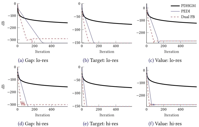
For our reporting, we computed a target optimal solutionbxby taking one million iterations of the basic PDHGM. In Figure 1and Table 1for TV denoising, andFigure 2and Table 2for
H1 denoising, we report the following: the distance tobx in decibels10 log10(kxi −bxk2/kbxk2),
the primal objective value val(x) := G(x) + F(Kx) relative to the target 10 log10((val(x) − val(xˆ))2/val(xˆ)2), as well as the duality gap10 log10(gap2/gap20), again in decibels relative to the initial iterate. For forward–backward splitting, to compute the duality gap, we solve the primal variablexifrom the primal optimality conditionK∗yi =∇G(xi)=xi−z.
5.3 performance analysis and concluding remarks
As expected, the performance of PEDI on TV denoising is not particularly good, reflecting the
O(1/N)rates fromTheorem 4.3. ForH1 denoising we observe significantly improved conver-gence, reflecting the linear rates from Theorem 4.5, and of dual forward–backward splitting. While PEDI eventually has better gap behaviour than dual forward–backward splitting, overall, however, the method appears no match for the latter in our sample problems. Further research is required to see whether there are problems for which the overall Primal Euclidean(Proximal)– Dual Interior or similar approaches provide competitive algorithms.
0 200 400 −150 −100 −50 0 Iteration d B
(a)Gap: lo-res
0 200 400
−100
−50 0
Iteration
(b)Target: lo-res
0 200 400
−100 −50 0 Iteration PDHGM PEDI Dual FB
(c)Value: lo-res
0 200 400
−150 −100 −50 0 Iteration d B
(d)Gap: hi-res
0 200 400
−80 −60 −40 −20 0 Iteration
(e)Target: hi-res
0 200 400
−100
−50 0
Iteration
[image:24.595.112.488.91.332.2](f)Value: hi-res
Figure 1:TV denoising convergence behaviour: high and low resolution images; gap, distance
to target solution, and primal objective value in decibels.
0 200 400
−300 −200 −100 0 Iteration d B
(a)Gap: lo-res
0 200 400
−150
−100
−50 0
Iteration
(b)Target: lo-res
0 200 400
−200 −100 0 Iteration PDHGM PEDI Dual FB
(c)Value: lo-res
0 200 400
−300 −200 −100 0 Iteration d B
(d)Gap: hi-res
0 200 400
−150
−100
−50 0
Iteration
(e)Target: hi-res
0 200 400
−200
−100 0
Iteration
(f)Value: hi-res
Figure 2:H1 denoising convergence behaviour: high and low resolution images; gap, distance
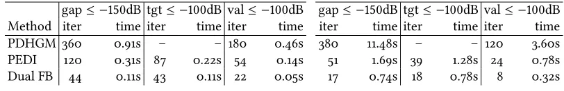
[image:24.595.111.491.391.633.2]Table 2:H1 denoising performance: CPU time and number of iterations (at a resolution of 10) to reach given duality gap, distance to target, or primal objective value.
low resolution
gap≤ −150dB tgt≤ −100dB val≤ −100dB Method iter time iter time iter time
PDHGM 360 0.91s – – 180 0.46s
PEDI 120 0.31s 87 0.22s 54 0.14s
Dual FB 44 0.11s 43 0.11s 22 0.05s
high resolution
gap≤ −150dB tgt≤ −100dB val≤ −100dB iter time iter time iter time
380 11.48s – – 120 3.60s
51 1.69s 39 1.28s 24 0.78s
17 0.74s 18 0.78s 8 0.32s
acknowledgements
The final stages of this research have been performed with the support of the EPSRC First Grant EP/P021298/1, “PARTIAL Analysis of Relations in Tasks of Inversion for Algorithmic Leverage”.
a data statement for the epsrc
All data and source codes will be deposited for readers to access when the final accepted version of the manuscript is submitted.
references
[1] S. H. Schmieta and F. Alizadeh, Extension of primal-dual interior point algo-rithms to symmetric cones, Mathematical Programming 96 (2003), 409–438, doi:10.1007/s10107-003-0380-z.
[2] L. Faybusovich,Euclidean jordan algebras and interior-point algorithms, Positivity1(1997), 331–357, doi:10.1023/A:1009701824047.
[3] R. Monteiro,Polynomial Convergence of Primal-Dual Algorithms for Semidefinite Program-ming Based on the Monteiro and Zhang Family of Directions, SIAM Journal on Optimization 8(1998), 797–812, doi:10.1137/S1052623496308618.
[4] Y. E. Nesterov and M. J. Todd, Self-scaled barriers and interior-point methods for convex programming, Mathematics of Operations Research 22 (1997), 1–42, doi:10.1137/S1052623495290209.
[5] M. Grant and S. Boyd,CVX: Matlab software for disciplined convex programming, version 2.1,http://cvxr.com/cvx(2014).
[6] M. Grant and S. Boyd,Graph implementations for nonsmooth convex programs, in:Recent Advances in Learning and Control, Edited by V. Blondel, S. Boyd and H. Kimura, Lecture Notes in Control and Information Sciences, Springer-Verlag Limited2008, 95–110.
[8] I. Loris and C. Verhoeven, On a generalization of the iterative soft-thresholding al-gorithm for the case of non-separable penalty, Inverse Problems 27 (2011), 125007, doi:10.1088/0266-5611/27/12/125007.
[9] D. Gabay,Applications of the method of multipliers to variational inequalities, in:Augmented Lagrangian Methods: Applications to the Numerical Solution of Boundary-Value Problems, volume 15, Edited by M. Fortin and R. Glowinski, North-Holland1983, 299–331.
[10] A. Chambolle and T. Pock,A first-order primal-dual algorithm for convex problems with applications to imaging, Journal of Mathematical Imaging and Vision40(2011), 120–145, doi:10.1007/s10851-010-0251-1.
[11] B. He and X. Yuan,Convergence analysis of primal-dual algorithms for a saddle-point prob-lem: From contraction perspective, SIAM Journal on Imaging Sciences 5 (2012), 119–149, doi:10.1137/100814494.
[12] R. T. Rockafellar,Monotone operators and the proximal point algorithm, SIAM Journal on Optimization14(1976), 877–898, doi:10.1137/0314056.
[13] T. Valkonen and T. Pock,Acceleration of the PDHGM on partially strongly convex functions, Journal of Mathematical Imaging and Vision (2016), doi:10.1007/s10851-016-0692-2, to ap-pear,arXiv:1511.06566.
URLhttp://iki.fi/tuomov/mathematics/cpaccel.pdf
[14] T. Valkonen,Testing and non-linear preconditioning of the proximal point method (2017), submitted,arXiv:1703.05705.
URLhttp://iki.fi/tuomov/mathematics/proxtest.pdf
[15] T. Valkonen,Block-proximal methods with spatially adapted acceleration(2016), submitted,
arXiv:1609.07373.
URLhttp://iki.fi/tuomov/mathematics/blockcp.pdf
[16] Z. Yu, Y. Zhu and Q. Cao,On the convergence of central path and generalized proximal point method for symmetric cone linear programming, Appl. Math. Inf. Sci.7(2013), 2327–2333, doi:10.12785/amis/070624.
[17] J.-S. Chen and S. Pan,An entropy-like proximal algorithm and the exponential multiplier method for convex symmetric cone programming, Computational Optimization and Appli-cations47(2010), 477–499, doi:10.1007/s10589-008-9227-0.
[18] J. López and E. A. P. Quiroz,Construction of proximal distances over symmetric cones, Op-timization (2017), doi:10.1080/02331934.2016.1277998, published online.
[19] A. Kaplan and R. Tichatschke,Interior proximal method for variational inequalities on non-polyhedral sets, Discussiones Mathematicae, Differential Inclusions, Control and Optimiza-tion27(2007), 71–93, doi:10.7151/dmdico1077.
[21] D. Boley, Local linear convergence of the alternating direction method of multipliers on quadratic or linear programs, SIAM Journal on Optimization 23 (2013), 2183–2207, doi:10.1137/120878951.
[22] D. Han and X. Yuan,Local linear convergence of the alternating direction method of multi-pliers for quadratic programs, SIAM Journal on Numerical Analysis51(2013), 3446–3457, doi:10.1137/120886753.
[23] M. Hong and Z.-Q. Luo,On the linear convergence of the alternating direction method of mul-tipliers, Mathematical Programming162(2017), 165–199, doi:10.1007/s10107-016-1034-2.
[24] J. Liang, J. Fadili and G. Peyré,Local linear convergence of forward–backward under partial smoothness, Advances in Neural Information Processing Systems27(2014), 1970–1978.
URLhttp://papers.nips.cc/paper/5260-local-linear-convergence-of-forward-backward-under-partial-smoothness.p
[25] K. Bredies and D. A. Lorenz,Linear convergence of iterative soft-thresholding, Journal of Fourier Analysis and Applications14(2008), 813–837, doi:10.1007/s00041-008-9041-1.
[26] R. T. Rockafellar,Convex Analysis, Princeton University Press1972.
[27] J. Faraut and A. Korányi,Analysis on Symmetric Cones, Oxford University Press1994.
[28] M. Koecher,The Minnesota notes on Jordan algebras and their applications,Lecture Notes in Mathematics, volume 1710, Springer-Verlag, Berlin1999.
[29] L. Faybusovich, Linear systems in Jordan algebras and primal-dual interior-point algorithms, Journal of Computational and Applied Mathematics 86 (1997), 149–175, doi:10.1016/S0377-0427(97)00153-2.
[30] T. Valkonen,Diff-convex combinations of Euclidean distances: a search for optima, num-ber 99 in Jyväskylä Studies in Computing, University of Jyväskylä2008, Ph.D Thesis. URLhttp://iki.fi/tuomov/mathematics/thesis.pdf
[31] S. J. Wright and D. Orban, Properties of the log-barrier function on degener-ate nonlinear programs, Mathematics of Operations Research 27 (2002), 585–613, doi:10.1287/moor.27.3.585.312.
[32] H. Ramírez and D. Sossa,On the central paths in symmetric cone programming, Journal of Optimization Theory and Applications (2016), 1–20, doi:10.1007/s10957-016-0989-8.
[33] J. X. da Cruz Neto, O. P. Ferreira, P. R. Oliveira and R. C. M. Silva,Central paths in semidefinite programming, generalized proximal-point method and cauchy trajectories in riemannian manifolds, Journal of Optimization Theory and Applications139(2008), 227, doi:10.1007/s10957-008-9422-2.