Progress Towards finding Quark Masses and the QCD scale Lambda from the Lattice

arXiv:hep-lat/0411036v1 25 Nov 2004

Progress Towards finding Quark Masses and the QCD scale Λ from the

Lattice

P.E.L. Rakowa a

Department of Mathematical Sciences, University of Liverpool, Liverpool L69 3BX, UK

We discuss recent work trying to extract the renormalised quark masses and Λ, the QCD scale, from dynamical simulations in lattice gauge theory.

1. INTRODUCTION

Quark masses and ΛQCD are both parameters

which are not accessible to direct observation, un-like quantities such as hadron masses which have a very clear meaning both in the continuum and on the lattice. Extraction of either quantity from lattice data inevitably involves both a matching of lattice measurements with continuum measure-ments and the use of results from perturbation theory.

We can divide the reliance on perturbation the-ory into two classes. In the most favourable cases all the perturbation theory needed can be per-formed in the continuum. In this case the technol-ogy of perturbation theory is very well-developed, and we can expect to find fairly long perturbative series (often to three loops) for the quantities we need. Less favourable is the case when lattice perturbation theory is needed. The propagators and vertices for lattice perturbation theory are much more complicated, making high order cal-culations very difficult. However we will see that some impressive progress is being made with lat-tice perturbation theory too.

The structure of this paper is as follows. First we will discuss renormalisation in general, as this is crucial to producing quark masses defined in a way that can be related to continuum physics. Then we will discuss quark masses, dealing sep-arately with the lighter quarks (up, down and strange) and (in less detail) with the heavier quarks (charm and bottom).

For the light quarks the method we discuss in most detail is the use of the pseudoscalar meson masses to determine the quark masses. From the

lowest-order chiral perturbation theory we know that a pseudoscalar meson made of quarks of flavouraandbhas its mass given by

m2

P S∝ma+mb (1)

which implies that the pseudoscalar meson mass (and especially the πmass) will be very sensitive to the quark masses. Eq. (1) also implies that the average light quark mass ml ≡

1

2(mu+md)

will be easier to measure than the separateuand d masses, and in this contribution we will only discuss this averaged light quark mass.

In the second part of the paper we will dis-cuss attempts to fix the scale parameter of QCD, ΛQCD, both from measurements carried out at

“normal” lattice spacings, using gauge configura-tions generated for other projects, and from fine lattice spacings, using simulations dedicated to the purpose of determining Λ.

2. RENORMALISATION AND Z FAC-TORS

With very few exceptions, an operator expec-tation value measured on the lattice has to be renormalised before we can give a number which can be compared with experiment. One can think of this as a calibration factor. Estimating Zm,

the renormalisation factor for the quark mass, is one of the more difficult steps in the calculation of quark masses, so it is appropriate to discuss renormalisation in some detail.

There are a handful of cases where theZfactor is not needed (for example, the conserved vector current). In other cases one can do a completely

2

non-perturbative calculation. An example of this isZV, the renormalisation constant for the local

vector current, ψγµψ. We know, from the

con-servation of baryon number and charge, exactly what the correct answer should be when the ma-trix element of the vector current is measured in a hadron. This can be used to calculateZV, e.g. [1].

This calculation does not rely on any perturba-tion theory at all, neither on the lattice nor in the continuum.

Usually we are not this fortunate, and we have to calibrate our lattice probe by comparing lattice results with continuum perturbation theory re-sults [2]. To use this method one measures quark propagators and Greens functions at a range of virtualities. Because these are gauge-dependent quantities the gauge must be fixed, the usual choice is to impose the Landau gauge. The re-lation we use to define the renormalisation of an operatorO is

ΛM S

O =

ZO

Zψ

Λlat

O , (2)

where Zψ is the wave-function renormalisation

constant, defined in a similar fashion by compar-ing the lattice propagator with theM S propaga-tor1

.

Where do we get the M S Greens functions which we need for this calculation? Here we have to rely on continuum perturbation theory. The results we need to interpret our lattice results are now available up to 3 or 4 loops [3]. Even the continuum perturbation series can be slowly con-verging in some cases. Tricks to accelerate the se-ries’ convergence, such as careful choice of scale, may be helpful.

The comparison between lattice and continuum results must be performed at a scaleµ that sat-isfies

Λ2

QCD≪µ

2

≪1/a2

. (3)

1_{Traditionally the process is split up into two stages by} introducing an intermediate renormalisation scheme such as RI or RI′_{. A renormalisation factor taking us from}

lattice to RI′ _{is followed by a conversion factor to change}

RI′_toM S. I think the nature of the calculation is easier to follow if we combine both stages, and convert directly from lattice toM S.

The lower limit arises because when µ2

is too small we do not know the true value of ΛM S

O ,

since our perturbative series do not converge fast enough, and because the Greens function may have large non-perturbative contributions, for ex-ample contributions associated with the sponta-neous breaking of chiral symmetry and the ex-istence of a quark condensate. The upper limit arises because the lattice Greens function will have discretisation errors which become impor-tant when a2

µ2

∼1. The method of [2] relies on the existence of a plateau region between these two limits, and in practice this may turn out to be disappointingly narrow.

There is little that can be done about the lower limit, what happens here is a real physical effect, present both on the lattice and in the continuum. On the other hand lattice perturbation theory can be used to greatly reduce thea2

µ2

errors, extend-ing the useful plateau region outwards.

Normally lattice perturbation theory results are quoted for small external momentaa2

µ2

≪1 but with a little extra effort the Greens functions can be found for any external momentum. Sub-tracting off the one-loop contribution to the dis-cretisation errors allows us to reduce errors of this type from O(g2

a2

µ2

) to O(g4

a2

µ2

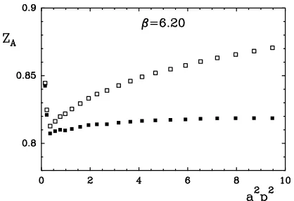
). The success of this procedure can be seen in Fig. 1, which shows a much better plateau after subtraction of one-loop lattice artefacts.

2.1. Singlet Contribution

We have discussed how to measure the renor-malisation constants for quark bilinear operators, but how can we measure the mass renormalisation factor Zm? The usual method is to look for an

identity relating Zm to ZS, the renormalisation

factor for the scalar operator.

The usual way to derive this is by looking at the divergence of a flavour non-singlet vector current Ja

µ. In the continuum this current is ψγµτaψ,

where τ is a traceless flavour matrix. The lattice form depends on the fermion action, for Wilson or clover fermions it is

1

2ψ(x+ ˆµ)[γµ+r]τ

a_ψ(x)

+1

2ψ(x)[γµ−r]U

Figure 1. The renormalisation factor for the axial current, for quenched clover fermions at β = 6.20. The open squares show the raw data, the black squares show the result after subtraction of the one-loop discretisation errors. The subtrac-tion procedure increases the plateau region.

The Ward identity [4] reads

∂µJµa

=

ψ [M, τa_{] ψ}

+ contact terms, (4) where M is the quark mass matrix. This iden-tity links the flavour non-singlet scalar operator and the flavour non-singlet part of the mass ma-trix. Eq. (4) is an exact lattice identity if we use the conserved vector current, but because it only involves the non-singlet part of the mass matrix (i.e. mass differences), it still permits an additive renormalisation of the singlet part of the mass matrix (which does of course occur in Wilson or clover fermions).

Requiring that eq. (4) still hold after renormal-isation tells us that ZN S

m Z_ψψN S = 1. This tells us

how to renormalise non-singlet quantities, such as mass differences, but it doesn’t tell us how the singlet part ofM (which commutes withτ) renor-malises.

InM S we are used to having a difference be-tween singlet and non-singlet renormalisation fac-tors for operafac-tors with anoddnumber of gamma matrices. Because clover fermions have no ex-act chiral symmetry, there can be a difference be-tween singlet and non-singletZfor operators with anevennumber of gamma matrices too. This can be seen in Fig. 2. In the continuum the “bubble”

diagram would be the product of 5 gamma matri-ces (3 from propagators, 2 from qqg vertices) so its trace would be zero in the massless case. For Wilson or clover fermions this no longer holds, and the bubble will give a non-zero contribution.

Figure 2. An example (above) of a Feynman dia-gram present in both singlet and non-singlet cases, and (below) a diagram which only contributes to the singlet Z. The black point shows where the ψψ operator is inserted.

The singlet vector current does not give us any useful information about the mass matrix, but we can find some relationships by considering partially quenched QCD, with valence quarks al-lowed to have a different mass from the sea quark mass. If we change the valence quark mass while keeping the sea quark mass fixed, the derivative of the quark propagator S gives the non-singlet scalar three-point function

∂ ∂ 1

2_κval

S(p) =GN S

ψψ(p). (5)

However if we change valence and sea quark masses together we get an identity for the singlet scalar three-point function

∂ ∂ 1

2_κval

+ ∂ ∂ 1

2_κsea

!

S(p) =GS_ψψ(p). (6)

From these identities we conclude that ZN S

4

Vector Ward Identity) and ZS

mZ_ψψS = 1 which

is new. We can findZN S

ψψ and thusZ N S m by the

non-perturbative methods discussed earlier. The identities here also give us a way of findingZS

m.

Figure 3. Dynamical and partially quenched pseu-doscalar meson masses for clover fermions at β= 5.29. Data from [5].

In Fig. 3 we show partially quenched (open points) and full dynamical (filled points) data for the pseudoscalar meson masses. We can immedi-ately see that there is a different criticalκ if we follow the solid line connecting the full dynami-cal points (the points with valence and sea quark masses equal) than if we follow one of the dashed lines (sea quark mass held fixed, valence quark mass varied). This is because clover fermions have no exact chiral symmetry, and so an additive quark mass renormalisation is possible. The dif-ference in criticalκs shows that this additive term depends quite strongly on the sea quark mass.

In the continuum the situation would look quite different — because of chiral symmetry both the full and partially quenched curves would both have to pass through the origin, at zero valence quark mass. This would also apply for a lattice fermion formulation (such as overlap fermions) which have an exact chiral symmetry. After renormalisation the lattice results ought to show the same structure, with both full dynamical and

partially quenched mP S vanishing at the same

place. The only way to arrange this is to use different renormalisation factors for the partially quenched and full QCD quark masses, see Fig. 4, just as we expected from considering the identi-ties eqs. (5) and (6).

Figure 4. Dynamical and partially quenched pseudoscalar meson masses before and after renormalisation of the quark mass.

We define the bare sea and valence quark masses by

m= 1 2κ−

1 2κc

with κc defined as the critical κ for QCD with

equal valence and sea quark masses (see Fig. 4). The renormalised masses are then defined by

mRsea = ZmSmsea, (8)

mR

val = ZmN S(mval−msea) +ZmSmsea.

The partially quenched pseudoscalar mesons are massless at the point where mR

val= 0, which we

callκval

c . We can use this to find the ratio of the

twoZ’s, ZS m

ZN S m

= msea−mval msea

κval=κcval

(9)

=

₁

2κsea

− 1

2κc val

1 2κsea

− 1

2κc

−1

.

Z ratios calculated this way in [5] are shown in Fig. 5. The ratio only depends weakly on the quark mass, but it depends very strongly on β. The ratio drops rapidly as lattice spacing de-creases.

Figure 5. The ratioZS

m/ZmN Sfor dynamical clover fermions [5]. β values run from 5.20 (highest line) to 5.40 (lowest line).

One way to illustrate the importance of the ra-tioZS

m/ZmN Sis to go back to one of the pioneering

dynamical calculations [6], carried out with two

flavours of unimproved Wilson fermions. In this paper they initially found a value for the ratio ms/ml≈52, which is a long way from the value

found in quenched calculations, and also far from the predictions of chiral perturbation theory

ms

ml

= 2m

2

K−m

2

π

m2

π

≈25. (10)

Normally one would expect the mass renormalisa-tion factor to cancel out in this ratio, but because the singlet and non-singletZdiffer this is not en-tirely true.

In Fig. 6 we show a pion line, the line giv-ing the pseudoscalar mass when valence and sea quark masses are equal, and the kaon line, show-ing the result when sea quarks and one valence quark (representing theuordin theK) are kept at a fixed mass, while the other valence quark (representing the strange quark) is varied. The slopes of these two lines are different, just as seen in the partially quenched case.

Figure 6. A schematic diagram illustrating the subtleties of measuring the strange/light quark mass ratio from Wilson fermions.

6

crosses the mass-squared of the physical K. If we now use these two κ values to calculate the ratio of the bare quark masses, mbare

s /mbarel we

get a ratio much larger than from eq. (10), be-cause theK line in Fig. 6 is less steep than the πline. However, if we renormalise the masses ac-cording to eq. (8), then the slopes of the kaon and pion lines will become approximately equal, as in the lower panel of Fig. 4, and now the ratio of therenormalisedquark masses will be close to eq. (10).

0 1 2 3 4 5 6 7

0 0.1 0.2 0.3 0.4 0.5

a [GeV-1] m

— MS——

[MeV]

semi-quenched direkt

Figure 7. A figure from [7] showing the differ-ence in light quark masses found from partially quenched and fully dynamical (“direkt”) data.

In later works [7] the SESAM collaboration used a different strategy, measuring data from both partially quenched and fully dynamical mesons, and then making a joint extrapolation to the continuum limit, Fig. 7. The same Z was used in both cases. This gives a result more in line with what we do here, but it is not exactly the same. Although we have seen in Fig. 5 that the ratioZS

m/ZmN Sdecreases asadecreases, there

will presumably be a perturbative contribution at the two-loop level, which means that theZ ratio will asymptotically approach the value 1 rather slowly, like 1 +O(g4

), rather than like a power of

a, so one will not be able to completely remove this effect by power-law extrapolations ina.

The argument we give here, using different Z factors for the singlet and non-singlet parts of the mass matrix is rather similar to the discussion given at Lattice ’97 in [8].

2.2. Quark mass results

The preliminaries are now over, and it is time to discuss some of the recent quark mass results from dynamical simulations.

Figure 8. A comparison of quenched (above) and dynamical (below) estimates for the strange quark mass [5].

In Fig. 8 we show an estimate of the strange quark mass calculated using the flavour-singlet renormalisation constant calculated from the comparison of dynamical and partially quenched mesons. The result is rather similar to that found in the quenched case. If the non-singlet renormal-isation constant had been used thea-dependence would be much stronger, and the data points would have been lower.

with flavour indexa[4],

h∂µAaµi=hψ{m, τa}γ5ψi+contact terms. (11)

In clover fermions the axial current has to be im-proved by adding irrelevant operators, because of the lack of a true chiral symmetry. As can be seen from the Ward identity, this axial Ward identity (AWI) mass has to be renormalised by the factor

mren= ZA ZP

mAW I . (12)

The final renormalised result ought to be the same in either case, but we will see that this is not yet the case, there are still fairly large dif-ferences between different groups working on this problem.

The AWI quark mass definition has been used by the CP-PACS and JLQCD Collaborations to study the quark masses in clover QCD, both for two-flavour [9] and (2+1) flavour simulations [10]. The Z ratio needed to renormalise the bare lat-tice masses are calculated from tadpole-improved one-loop lattice perturbation theory. Their re-sults are summarised in Fig. 9. In the quenched case the result depends quite heavily on whether theKorφmeson is used to determine the strange quark mass. This is a sign that the quenched the-ory differs from the real world. Fortunately this discrepancy is greatly reduced when sea quarks are switched on, as can be seen in the panels of Fig. 9 showing thesquark mass from dynamical QCD.

The SPQcdR Collaboration [11] have measured quark masses in anNf = 2 simulation using the

Wilson quark action at a singleβ value,β = 5.8. They use both the VWI and AWI definitions of quark mass, and find compatible results from both methods. The renormalisation constants are found non-perturbatively using the method of [2]. Their preliminary values are included in Table 1, and are broadly compatible with the results of [5]. In [12] the quark masses are measured in a dynamical simulation with (2+1) flavours of sea quark. The use of staggered quarks speeds up the calculation considerably, allowing the light u/d sea quarks to be simulated all the way down to

2.0 3.0 4.0

mud

MS

(

µ

=2GeV)

N_f=2+1 N_f=2 N_f=0

a ~ 0.1 fm AWI

a ~ 0.1 fm a ~ 0.1 fm

RG + clover(PT) RG + clover(PT)

AWI AWI

K-input

φ-input RG + clover(NPT)

60 80 100 120 140 160

ms

MS

(

µ

=2GeV)

N_f=2+1 N_f=2 N_f=0

RG + clover(PT) RG + clover(PT)

a ~ 0.1 fm a ~ 0.1 fm

AWI AWI

RG + clover(NPT)

K-input

AWI a ~ 0.1 fm

φ-input

φ-input

K-input

φ-input

K-input

Figure 9. Theuanddquark masses (above) and s quark mass (below) ata∼0.1fm, from [10].

masses ∼ms/8, a considerable advance on what

is possible with other quark formulations. The staggered quarks have been improved to suppress ‘taste’ violation and other discretisation errors. This also has the effect of making perturbation theory better behaved than it is for unimproved staggered fermions. The Z factors used in [12] are calculated in one-loop tadpole improved per-turbation theory. The estimated error due to the unknown higher-order terms in perturbation the-ory is 9%. This study finds that the effects of including sea quarks are dramatic, and that the final physical masses of the quarks are a lot lighter in the dynamical simulation than they were in a quenched calculation.

8

ml/MeV ms/MeV sea quarks Reference

3.05(6) 80.4(1.9) (2+1) CP-PACS and JLQCD [10] 2.8(0)(1)(3)(0) 76(0)(3)(7)(0) (2+1) HPQCD, MILC and UKQCD [12]

4.7(2)(3) 119(5)(8) Nf = 2 QCDSF/UKQCD [5]

4.8(5) 111(6) Nf = 2 SPQcdR Collaboration [11]

4.5(17) Nf = 2 SESAM/TχL [7]

Table 1

Masses of the light, ml=

1

2(mu+md), and strange quarks in dynamical lattice QCD, as determined by

various collaborations. The masses are given in theM S scheme at a scale of 2 GeV.

{ 15{

Figure 2. The values of each quark mass parameter taken from

the 2004 Data Listings. The most recent data points are at the

top of each plot. Points from papers reporting no error bars are

open circles. Arrows indicate limits reported. The grey regions

indicate values excluded by our evaluations; some regions were

determined in part through examination of Fig. 1.

June 16, 2004 16:10

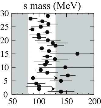
Figure 10. Determinations of the strange quark mass from the Particle Data Group [13].

Group [13]. Comparing this with Table 1 we see that most of the dynamical lattice determi-nations look low compared with estimates from traditional methods.

2.3. The charm quark mass

The charm quark mass has its own special dif-ficulties because mc is comparable with the

in-verse lattice spacing a−1

for the lattice spacings we have to work with at present. This means that lattice artefacts proportional to high powers of amc can be important, so it would be useful

to have expressions resumming all (amc)nterms.

Suggestions on how to do this (known as FNAL masses) were made in [14]. As the lattice spac-ing becomes smaller all definitions should agree. This is examined in [15], where the charm mass determined from the axial and vector Ward iden-tity definitions, and the mass determined from the FNAL method m1 and m2 are compared in

the quenched case (where the a range can be made large). At present lattice spacings the mass from the Axial Ward Identity (mA) looks as if it

might extrapolate to a lower value than the oth-ers, though there is still room for it to move up again, see Fig. 11.

This reference also looks at the effect of find-ing mc on dynamical clover configurations, the

open symbols on the right-hand side of Fig. 11. There seems to be very little difference between the quenched and dynamical results, though of course the present results are at a single rather coarse lattice spacing, and the sea quarks in the simulation are rather heavy.

2.4. b quark mass

A nice example of the interplay between pertur-bation theory and physical result is the b quark mass calculation of Gimenez, Giusti, Rapuano and Martinelli [16] converting lattice data into a value formbinM S, using stochastic perturbation

theory results from [17].

0 0.1 0.2 0.3 0.4 0.5

a (GeV)-1

0.9 1 1.1 1.2 1.3 1.4 1.5 1.6 1.7

mc

(m

c

) (GeV)

m_V m_A m₁ m₂

Figure 11. Different determinations of the charm quark mass [15]. The closed symbols show the effect of using different mass definitions in the quenched case. All definitions should lead to the same continuum value. The open symbols at the right show the charmed quark mass determined on Nf = 2dynamical configurations from UKQCD.

After that, the conversion from pole mass toM S mass is done using results from continuum per-turbation theory. Since the b quark pole mass is just used as an intermediate step the calculation taken as a whole is presumably legitimate even though confinement means that there is no pole in theb-quark propagator.

The two-loop subtraction for the residual mass was calculated using traditional lattice perturba-tion theory methods in [18]. The three-loop result was calculated using the novel method of stochas-tic perturbation theory, which has the major advantage that the difficulty of calculating new terms in the series does not increase as rapidly as it does in conventional calculations. Stochas-tic perturbation theory thus promises to over-take conventional techniques in the future. It does have some disadvantages, being a stochastic

method, the coefficients calculated do have a sta-tistical error, and can not be given to the number of decimal places that we are used to from con-ventional perturbation theory, but they are usu-ally quite good enough for comparison with real lattice data.

The dependence of the final b quark mass on the order of lattice perturbation theory used is illustrated in Table 2. Knowing the three-loop coefficient helps to significantly reduce the sys-tematic uncertainty in the final estimate, which is

mb(mb)|unq = (4.21±0.03±0.05±0.04) GeV.

3. DETERMINING Λ

An important (but difficult) project for the lat-tice is to link the low-energy, non-perturbative quantities we normally measure (such as hadron masses) with the high-energy world accessible in accelerators, where perturbative QCD works well. The key to bridging this gap is to find a value for Λ, the scale parameter of QCD.

The strategy for determining Λ has two nec-essary parts. Firstly some dimensionful quantity has to be measured to set the scale. A common choice is to look at the static potential. This can be measured fairly well. A good way to fix a length scale is to find the distance at which

r2

F(r)≡ −r2 d

drV(r) (13)

has a particular value [19], the usual value chosen is 1.65, which gives a distance scale r0 ≈0.5f m.

Another way to find a length scale from the po-tential, now less popular, would be to use the string tension.

Secondly, we need to extract theM S coupling at a known scale, which can then be converted into a value for Λ_{M S}. One possibility is to use lattice perturbation theory to relate the lattice couplingg2

= 6/β tog2

M S.

Relating the Λ parameters of two schemes is a finite calculation. This is an asymptotic state-ment, and can be answered completely by a one-loop calculation [20].

10

mb(mb) Dependence on higher orders (unquenched data)

Order δm mpole_b mb(mb)/mpoleb mb(mb) ∆mb

LO 0 3770 1.000 3770 –

NLO 978.79 4748.79 0.92276 4382 612 NNLO 10.53 4759.32 0.89060 4239 143 NNNLO 74.55 4833.87 0.86883 4200 39 Table 2

A table illustrating the way in which the estimate for the bottom quark mass mb(mb) depends on the order of the lattice perturbation theory used. The quark mass results are preliminary values from [16], using perturbative calculations from [17] and [18].

asymptotic regime we need calculations of theβ -function of both schemes to as high an order as possible, this can then be translated into a rela-tion between the couplings. Currently we know the latticeβ function to three loops [21].

As often happens with lattice perturbation the-ory we find that the series converge rather poorly. Fortunately we have several methods to accel-erate the convergence. One explanation for the large coefficients in lattice perturbation theory is that they come from gluon “tadpoles” due to the higher order vertices present on the lat-tice [22]. A way to take these into account is to re-express the series in terms of a “boosted” cou-pling,g2

=g

2

/Uplaq_:

1 g2

M S(

1

a)

= 1

g2−0.4682013−0.0556675g 2

,

1 g2

M S(

1

a)

= 1 g2

−0.1348680−0.0217565g2

,

1 g2

M S(

2.63

a )

= 1 g2

−0.013837g2

. (14)

Using the quenched case as an example we can see in the equation above that the coefficients in the series for the M S coupling are reduced when we change the expansion parameter fromg2

to g2

.

We can improve the series further by choosing a natural scale [23]. If, instead ofg2

M S(1/a) we

cal-culate g2

M S(2.63/a), the g

0

term vanishes, and

the first correction is O(g2

) with a rather small

coefficient. This gives us grounds to hope that the unknown higher-order coefficients will not se-riously change the estimate ofg2

M S.

Once we have values for g2

M S we can use the

known β function to convert these into a value for ΛM S_{. The results in the quenched case [24],}

based on data from [25] and [26], are shown in Fig. 12.

0.00 0.01 0.02 0.03 0.04 0.05

(a/r0)2

0.50 0.55 0.60 0.65

r0

Λ

MS

−−

Figure 12. ΛM S _{calculated for quenched QCD} for β values in the range 5.95 to 6.92 [24]. The r0 values for high β are from [26]. The data

ex-trapolates very smoothly towards a valueΛM S Nf=0=

242(11)(10)M eV.

Some extrapolation in a is needed, this seems not to present any great problem, the data look surprisingly linear ina2

, and the smallestavalues are close to the continuum limit. The result in physical units is ΛM S

Nf=0= 242(11)(10)M eV. The

first error is a statistical error, the second error is an attempt to estimate the possible effects of the unknown higher order terms in theβ functions.

configura-tions produced by the UKQCD/QCDSF Collab-orations. The latticeβ function for clover quarks is available [21]. In the dynamical case we need a double extrapolation, both in lattice spacing and in sea quark mass. Both these extrapola-tions are over a rather large distance. A simple phenomenological extrapolation formula is

r0ΛM S=const+B(a/r0) 2

+Camq+Dr0m_q .

(15) The formula fits the data fairly well, as can be seen in Fig. 13.

0.00 0.01 0.02 0.03 0.04 0.05

(a/r0)2

0.45 0.50 0.55 0.60

0.0 0.1 0.2 0.3 0.4 0.5

0.45 0.50 0.55 0.60

r0mq

r0ΛMS

−−

− B(a/r0)2 − Camq

r0ΛMS

−−

− Camq − Dr0mq

Figure 13. Extrapolation of ΛM S _for dy-namical quarks. The data are measured on UKQCD/QCDSF configurations with dynamical clover fermions [24]. The upper part of the figure shows the mass dependence after the data has been extrapolated to the continuum limit. The lower half shows the adependence of data after extrap-olating to the chiral limit.

The extrapolated value hasn’t changed very much due to the jump to finer lattice spacings in the past year [24], the new value is Λ = 222(4)(28)M eV atNf = 2.

0.45 0.5 0.55 0.6 0.65 0.7 0.75

0 0.02 0.04 0.06 0.08 0.1 0.12

ΛMS

r0

(a/r₀)2 SW-I Wilson KS SW

Figure 14. A comparison of continuum extrapola-tions ofr0ΛM S[27] made for various fermion

ac-tions. Wilson fermions are extrapolated linearly in a, while clover and staggered are extrapolated linearly in a2

.

One way to estimate the systematic error in the final result is to repeat the calculation for different formulations of dynamical fermions, and see how much the results scatter. A very complete study was carried out in [27]. As can be seen in Fig. 14 the results do still depend quite a lot on the action and extrapolation procedure. The dependence on the action could be due in part to higher order terms in the perturbation series, which will of course depend on the fermions used. A very impressive attack on finding Λ was re-ported in this year’s Lattice Conference [28], ex-tending work done in [29] with Asqtad improved staggered fermions. Extensive three-loop calcula-tions of Wilson loops and the static potential have been carried out. Some idea of the work involved can be gained by looking at the number of Feyn-man diagrams that have to be considered, Fig. 15. Wilson loops of different sizes are dominated by gluons of different virtualities, with small loops corresponding to large Q2

. Thus by calculating αs from loops of different sizes one can see how

αsruns even from data taken at a single value of

12

BD5 BD6 BD7 BD8

BD9 BD10 BD11 BD12

BD13 BD14 BD15 BD16

BD17 BD18 BD19 BD20

BD21 BD22 BD23 BD24a

BD24b BD25 BD26 BD27

BD28 BD29 BD30 BD31

BD32 BD33 BD34 BD35

Figure 15. The gluon and ghost Feynman dia-grams used in [28] to calculate three-loop results for Wilson loops and the static potential. A simi-lar number of fermion loop diagrams is needed to calculate the unquenched case.

In Fig. 17 we see the lattice results extrapolated out to the scale mZ, where they are compared

with the traditional Particle Data Group value. The agreement looks impressively good.

Is there any way of diminishing the dependence on high-order perturbation theory? The obvious way to reduce our sensitivity to high order terms in the perturbation theory is to work at weaker values of the coupling — in QCD this means working at high energy or short distance. This

0.15 0.2 0.25 0.3 0.35 0.4 0.45 0.5 0.55 0.6 0.65

1 2 3 4 5 6 7 8

alpha

V

q* in GeV Running of alpha

PDG value Fine MILC Configs Coarse MILC Configs Potential (Coarse)

Figure 16. The running of αs as determined by [28]. αs is defined in the potential scheme.

quires a very fine lattice spacing,a, which in turn forces us to consider simulations in small physi-cal volumes. The small volumes involved in this method mean that it isn’t possible to reuse config-urations generated for other projects on hadronic physics, the calculations require many dedicated runs at very largeβ values.

The ALPHA Collaboration have been pursu-ing this method for many years [30], uspursu-ing the same methods that they applied in the quenched case [31]. A recent plot of their results is shown in Fig. 18. By repeatedly halving the lattice spac-ing (and the physical size L of their system), they make measurements ofαsover a large range

of scales (more than two orders-of-magnitude). These are compared with the running expected from the three-loop β function. The data reach αsvalues∼0.1, where we are very confident that

log(1×1)

log(1×2)

log(1×3)

log(2×2)

log(1×2/u6

P)

log(1×3/u8

P)

log(2×2/u8

P)

log((1×1)(2×2)/(1×2)2

)

log(1×3/2×2)

V(r≤3/a)

Lattice Results Compared With PDG

α_{M S}(MZ)

0.12 0.115

0.11 0.105

Figure 17. αs(mZ)estimated from Wilson loops of various sizes, and from the short distance po-tential [28].

10 or 20, but clearly the precision that will be achieved from data at µ/Λ ∼ 1000 should be much greater.

This work has not yet given a final value for Λ in physical units, preliminary results give the value ln(ΛLmax) = −1.34(7) where αs(Lmax) =

0.372, but the final step is still needed, a con-version from the length scale they use, Lmax, to

physical units.

4. CONCLUSIONS

The determination of quark masses is the more mature of the two fields we have looked at. We see that agreement has not yet been reached, and there are still differences between the measure-ments of the different groups. It is not yet clear (to me at least) where the origin of these differ-ences lies, as there are many differdiffer-ences between the calculations, particularly in the ways the Z factors are calculated and in the choice of mass definition.

Figure 18. The running ofαs in two-flavour dy-namical QCD as determined by the ALPHA Col-laboration [30].

One area in which we are making progress, and can expect more advances in the coming years, is bringing the sea quark masses down towards more realistic values. When simulations are carried out with large sea quark masses it can be difficult to find much difference from quenched calculations, and the extrapolation to the physical region can be difficult. Now, with more powerful machines and new fermion actions, we are seeing simula-tions carried out much closer to the physical re-gion, and we can expect more soon.

A topic which we have not covered here is the calculation of quark masses using overlap fermions, since dynamical overlap is not yet as ad-vanced as dynamical calculations with the older fermion formulations.

14

complicated Feynman rules, and because there is now far greater diversity in the choice of fermion and gauge actions used. At Lattice ’04 we have seen that diagrammatic techniques are rising to the challenge, we have also seen that stochas-tic perturbation theory is delivering results which are useful to those extracting physics from lattice simulations.

REFERENCES

1. T. Bakeyev, M. G¨ockeler, R. Horsley, D. Pleiter, P.E.L. Rakow, G. Schierholz and H. St¨uben (QCDSF-UKQCD Collaboration), Phys. Lett. B580(2004) 197.

2. G. Martinelli, C. Pittori, C.T. Sachrajda, M. Testa and A. Vladikas, Nucl. Phys. B445 (1995) 81.

3. K.G. Chetyrkin and A. Retey, Nucl. Phys. B 583(2000) 3; J.A. Gracey, Nucl. Phys. B662 (2003) 247; Nucl. Phys. B667(2003) 242. 4. I. Montvay and G. M¨unster, “Quantum Fields

on a Lattice”, Cambridge University Press (1994).

5. M. G¨ockeler, R. Horsley, A.C. Irving, D. Pleiter, P.E.L. Rakow, G. Schierholz and H. St¨uben, arXiv:hep-ph/0409312.

6. N. Eickeret al.[SESAM Collaboration], Phys. Lett. B407(1997) 290.

7. N. Eickeret al.(SESAM/TχL Collaboration) Nucl. Phys. Proc. Suppl.106(2002) 209. 8. T. Bhattacharya and R. Gupta, Nucl. Phys.

Proc. Suppl.63(1998) 95.

9. A. Ali Khanet al.[CP-PACS Collaboration], Phys. Rev. D 65 (2002) 054505. [Erratum-ibid. D67(2003) 059901].

10. T. Ishikawa et al., (CP-PACS and JLQCD Collaborations) [arXiv:hep-lat/0409124]. 11. D. Becirevicet al., (SPQcdR Collaboration),

arXiv:hep-lat/0409110.

12. C. Aubin et al. (HPQCD, MILC and UKQCD Collaborations) Phys. Rev. D70 (2004) 031504; C. Aubin et al. (MILC Col-laboration), arXiv:hep-lat/0407028.

13. S. Eidelman et al., Phys. Lett. B592, 1 (2004).

14. B.P.G. Mertens, A.S. Kronfeld and A.X. El-Khadra, Phys. Rev.D58(1998) 034505.

15. A. Dougal, C.M. Maynard and C. McNeile, arXiv:hep-lat/0409089.

16. V. Gimenez, personal communication. 17. F. Di Renzo and L. Scorzato,

arXiv:hep-lat/0410010.

18. G. Martinelli and C.T. Sachrajda, Nucl. Phys. B 559(1999) 429.

19. R. Sommer, Nucl. Phys. B411(1994) 839. 20. A. Hasenfratz and P. Hasenfratz, Phys. Lett.

B93 (1980) 165; A. Hasenfratz and P. Hasen-fratz, Nucl. Phys. B 193 (1981) 210; P. Weisz, Phys. Lett. B 100 (1981) 331; R. Dashen and D.J. Gross, Phys. Rev. D 23 (1981) 2340.

21. C. Christou, A. Feo, H. Panagopoulos and E. Vicari, Nucl. Phys. B 525 (1998) 387 [Erratum-ibid. B 608 (2001) 479]; A. Bode and H. Panagopoulos, Nucl. Phys. B 625 (2002) 198.

22. G.P. Lepage and P.B. Mackenzie, Phys. Rev. D 48, 2250 (1993).

23. M. L¨uscher, arXiv:hep-lat/9802029.

24. M. G¨ockeler, R. Horsley, A.C. Irving, D. Pleiter, P.E.L. Rakow, G. Schierholz, H. St¨uben, (QCDSF-UKQCD Collabora-tion), arXiv:hep-lat/0409166.

25. S. Boothet al. (QCDSF-UKQCD Collabora-tion), Phys. Lett. B519(2001) 229.

26. S. Necco and R. Sommer, Nucl. Phys. B 622 (2002) 328.

27. G. Bali and P. Boyle, arXiv:hep-lat/0210033. 28. Q. Mason, these proceedings.

29. C. Davieset al., (HPQCD and UKQCD Col-laborations) Nucl. Phys. Proc. Suppl. 119 (2003) 595

30. A. Bode et al., Phys. Lett. B 515 (2001) 49; M. Della Morte et al., Nucl. Phys. Proc. Suppl. 119(2003) 439.