arXiv:1310.7898v1 [cs.DS] 29 Oct 2013
Moving in temporal graphs with very sparse
random availability of edges
Paul G. Spirakisa,b, Eleni Ch. Akridac
a
Computer Technology Institute & Press Diophantus (CTI), Patras, Greece
b
Department of Computer Science, University of Liverpool, UK
c
Department of Mathematics, University of Patras, Greece Email: spirakis@ cti. gr, akridel@ master. math. upatras. gr
Abstract
In this work we consider temporal graphs, i.e. graphs, each edge of which is assigned a set of discrete time-labels drawn from a set of integers. The labels of an edge indicate the discrete moments in time at which the edge is available. We also consider temporal paths in a temporal graph, i.e. paths whose edges are assigned a strictly increasing sequence of labels. Furthermore, we assume the uniform case (UNI-CASE), in which every edge of a graph is assigned exactly one time label from a set of integers and the time labels assigned to the edges of the graph are chosen randomly and independently, with the selection following the uniform distribution. We call uniform random temporal graphs the graphs that satisfy the UNI-CASE. We begin by deriving the expected number of temporal paths of a given length in the uniform random temporal clique. We define the term temporal distance of two vertices, which is the arrival time, i.e. the time-label of the last edge, of the temporal path that connects those vertices, which has the smallest arrival time amongst all temporal paths that connect those vertices. We then propose two statistical properties of temporal graphs. One is the maximum expected temporal distance which is, as the term indicates, the maximum of all expected temporal distances in the graph. The other one is the temporal diameter which, loosely speaking, is the expectation of the maximum temporal distance in the graph. Since uniform random temporal graphs, except for the clique, have at least a pair of vertices whose temporal distance is infinity, we assume the existence of aslow way to go directly from any vertex to any other vertex in order for the above measures to have a finite value. We derive the maximum expected temporal distance of a uniform random temporal star graph as well as an O(√nlog2n) upper bound, and a
greedy algorithm which computes in polynomial time the path that achieves it, on both the maximum expected temporal distance and the temporal diameter of the normalized
version of the uniform random temporal clique, in which the largest time-label available equals the number of vertices. Finally, we provide an algorithm that solves an optimization problem on a specific type of temporal (multi)graphs of two vertices.
1. Introduction
A temporal graph (or otherwise called temporal network) is, loosely speak-ing, a graph that changes with time. This concept incorporates a variety of both modern and traditional networks such as information and communica-tion networks, social networks, transportacommunica-tion networks, and several physical systems. The presence of dynamicity in modern communication networks, i.e. in mobile ad hoc, sensor, peer-to-peer, and delay-tolerant networks, is of-ten very strong. We can also find that kind of dynamicity in social networks, where the topology usually represents the social connections between a group of individuals. Those connections change as the social relationships between the individuals or even the individuals themselves change. Temporal graphs can also be associated with transportation networks. In a transportation network, there is usually some fixed network of routes and a set of trans-portation units moving over these routes. In such networks, the dynamicity refers to the change of positions of the transportation units in the network as time passes. Concerning physical systems, dynymicity may be present in systems of interacting particles.
In this work, embarking from the foundational work of Kempe et al. [KKK00], we consider the time to be discrete, that is, we consider networks in which changes can only occur at discrete moments in time, e.g. days or hours. This choice not only gives to the resulting models a purely combinatorial flavor but also naturally abstracts many real systems. In particular, we consider those networks that can be described via an underlying graph G
would mean that it is possible to transmit a data packet along the network nodes that belong to such a path from the first node in order to the last one, as time progresses. The time label on the last edge of a temporal path is called its arrival time and, in the above example of a connection network, it would indicate the time at which the transmitted data packet would arrive at the last node of the path.
In this work, we initiate the study of temporal graphs from a probabilistic and statistical viewpoint. In particular, we consider the case in which every edge of a graph is assigned exactly one time label from a setL0 ={1,2, . . . , a}
of integers. The time labels assigned to the edges of the graph are chosen randomly andindependently from one another from the setL0 and the
prob-ability that an edge is assigned a time label i ∈ L0 is equal to 1a, for every
i ∈ L0. We use the term UNI-CASE for the above described case and for
any graph that satisfies UNI-CASE’s properties we use the term Uniform Random Temporal Graph. We focus on examining three statistical proper-ties of such graphs. The first one, called expected number of temporal paths of a given length, is the number of temporal paths, of a given length, that we expect to have in a graph, given that every edge is assigned a label satisfying UNI-CASE. The second one, called the Maximum Expected Temporal Dis-tance, is the maximum of all temporal distances in the graph. By temporal distance of two vertices we denote the arrival time of the temporal path that connects those vertices, which has the smallest arrival time amongst all tem-poral paths that connect those vertices. The last property that we examine is calledthe Temporal Diameter of a uniform random temporal graph. Loosely speaking, it is the expected value of the maximum temporal distance in the graph, which of course is in correspondence with the diameter of a graph, as we know it up to now.
The motivation of the definitions we initiate and the work we carry out here comes from the natural question on how fast we can visit a particular destination, i.e. arrive at a particular network node, starting from a given point of origin, i.e. another network node, when the connection between a pair of nodes only exists at one moment in time.
1.1. Related work
labeled graphs that we study are naturally temporal properties. However, we can note that any property of a graph that is assigned labels from a discrete set of labels can correspond to some temporal property. Take for example a proper edge-coloring in a graph, i.e. a coloring of the graph’s edges in which no two adjacent edges have the same color. This corresponds to a temporal graph in which no two adjacent edges have the same time label, that is no two adjacent edges exist at the same time.
Single-labeled and multi-labeled Temporal Graphs. The model of temporal graphs that we consider in this work has a direct relation with the single-labeled model studied in [KKK00] as well as the multi-labeled model studied in [MMCS13]. The main results of [KKK00] and [MMCS13] have to do mainly with connectivity properties and/or cost minimization parameters for temporal network design. In this work we study temporal graphs from a statistical view and mainly focus on how fast we expect to arrive at a target vertex in a temporal graph. In [KKK00], a temporal path is considered to be a path with non-decreasing labels on its edges. In this work, we follow the assumption of [MMCS13] and consider a temporal path to be a path with strictly increasing labels. This choice is also motivated by recent work on dynamic communication systems, in which if it takes one time unit for the transmition of a data packet over a link, then a packet can only be transmitted over paths with strictly increasing labels.
Continuous Availabilities (Intervals). Some authors have assumed the availability of an edge for a whole time-interval [t1, t2] or multiple such
time-intervals. Although this is a clearly natural assumption, in this work we focus on the availability of edges at discrete moments and we design and develop techniques which are quite different from those needed in the continuous case.
1.2. Roadmap and contribution
In Section 2, we formally define the model of temporal graphs under con-sideration and provide all further necessary basic definitions. In Section 3, we make some general remarks on the expected number of temporal paths in any graph and proceed to the study of the expected number of temporal paths of a given length in the uniform random temporal clique ofn vertices,
Kn. For this matter, we distinguish two cases. In Section 3.1, we study the first case, where we set the largest label available for assignment to be
a =n−1 and we search for the expected number of temporal paths of length
of length k < a, when the largest label available for assignment is a=n−1. In Section 4, we formally define the maximum expected temporal distance of a uniform random temporal graph and we make some preliminary notations. In Section 4.1, we look at some known graphs’ maximum expected temporal distance. In particular, in Section 4.1.1, we study the case of the uniform random temporal star graph and we provide its exact maximum expected temporal distance. In Section 4.1.2, we study the case of the uniform ran-dom temporal clique, focusing on its normalized version, where the largest label, a, available for assignment is equal to the number of vertices, n. We also give a simple (greedy) algorithm which can, with high probability, find a temporal path with small expected arrival time from a given source to a given target vertex in the normalized uniform random temporal clique. In Section 5, we formally define the temporal diameter of a uniform random temporal graph and provide an inequality relation between the latter and the maximum expected temporal distance as well as the relevant proof. Fur-thermore, we provide an upper bound for both the temporal diameter and the maximum expected temporal distance of the nomalized uniform random temporal clique. In Section 6, we study an optimization problem on a specific type of temporal (multi)graphs of two vertices. We prove that the problem can by polynomially solved and provide an algorithm that gives the solution, along with the proof of its correctness. Finally, in Section 7 we conclude and give further research horizons opened through our work.
2. Preliminaries
Definition 1. A temporal graph is an ordered triplet G={V, E, L}, where:
• V stands for a nonempty finite set (called set of vertices)
• E stands for a set of m elements, each of which is a 2-element subset of V (called set of edges), and
• L = {Le,∀e ∈ E} = {Le1, Le2, . . . , Lem}, is a set of m elements,
Lei, 1 ≤ i ≤ m, each of which is a set of positive integers mapped
to the edge ei ∈ E (called assignment of time labels or simply assign-ment)
We also denote the temporal graph G = {V, E, L} by G′(L) or (G′, L),
where G′ = {V, E} is the graph, on the edges of which we assign the time
The values assigned to each edge of the graph are called time labels of the edge and indicate the times at which we can cross it (from one end to the other).
2.1. Further Definitions
We can now talk about temporal edges (or time edges) that are considered to be triplets (u, v, l), whereu, vare the ends of an edge in the temporal graph and l∈L{u,v} is a time label of this edge. That is, if an edge e={u, v} has
more than one time labels, e.g. has a set of three time labels,Le ={l1, l2, l3},
then this edge has three corresponding time edges, (u, v, l1), (u, v, l2) and
(u, v, l3).
Definition 2. A journey j from a vertex u to a vertex v ((u, v)- journey) is a sequence of time edges (u, u1, l1), (u1, u2, l2), . . . , (uk−1, v, lk), such that
li < li+1, for each 1≤i≤k−1.
We call the last time label of journey j, lk, arrival time of the journey. Definition 3. A (u, v)-journeyj in a temporal graph is called foremost jour-ney if its arrival time is the minimum arrival time of all (u, v)-journeys’ arrival times, under the labels assigned on the graph’s edges.
Now, consider any temporal graphG={V, E, L}. Let every edge receive exactly one time label, chosen randomly, independently of one another from a set L0 = {1,2, . . . , a}, where a ∈N, with the probability of an edge label
to be i, ∀i∈L0, equal to 1a. (UNI-CASE)
Definition 4. A temporal graph that satisfies UNI-CASE is called Uniform Random Temporal Graph (U-RTG).
In the special case, where the largest label,a, that can be assigned to the edges of a graph is equal to the number of its vertices, the graph is called Normalized Uniform Random Temporal Graph (Normalized U-RTG).
Note. There could be prospective study of cases in which each edge of a graph may receive several time labels, selected randomly and independently of one another from the setL0={1,2, . . . , a}, wherea∈N, with the selection
following a distribution F. (F-CASE)
In such cases, the graphs under consideration would be called F-Random Temporal Graphs (F-RTG) respectively.
of brevity, we often call such journeys “k edges temporal paths”. We also study the Expected (or Temporal) Diameter and the Maximum Temporal Distance of a graph, as defined in the following paragraphs.
3. Expected number of temporal paths
In this section we will search for the expected number ofk edges temporal paths in a clique of n vertices, Kn, that satisfies UNI-CASE.
It is obvious that for there to exist a temporal path of length k in any graph, the number of edges, k, has to be at most equal to the maximum label of the set L0, a, that can be assigned to the various edges. Otherwise, it is
impossible for a k edges temporal path to exist (see Figure 1).
L0 ={1,2,3(=a)}
k= 4
1 2 3 ;
Figure 1: There is no temporal path, when k > a
3.1. Special case: G=Kn, k =n−1, a=n−1
Initially, we focus our interest in the case of the clique (complete graph) of n vertices, Kn, that satisfies UNI-CASE with a = n−1 (i.e. with L0 =
{1,2, . . . , n− 1}), in which we seek the expected number of n − 1 edges
temporal paths.
Obviously, there can only be one assignment of labels of L0 on the k =
n−1 edges of any path starting from a random initial vertice v0 ∈ V(Kn)
in the clique Kn such, that we can find a journey on the edges of this path. This assignment gives label 1 on the 1st edge, label 2 on the 2nd edge, . . . , label n−1 on the (n−1)th edge.
is:
#assignments= (n−1)n−1
Consequently, given a path ofn−1 edges starting fromv0, the probability
for there to exist the corresponding temporal path (i.e. the one arising on the simple path after the assignment of the time labels) is:
P(temporal path of length n−1 starting f rom v0) =
1 (n−1)n−1
The number of paths of length n−1, starting from v0 in the clique Kn is equal to the number of permutations of the n−1 vertices remaining (i.e. except the start v0) to construct such a path. That is, the number of paths
of length n−1 that start from v0 in the clique Kn is:
(n−1)!
Therefore, since the clique Kn has n vertices, and due to the linearity of expectation, the expected number of temporal paths of length k = n−1 in the clique Kn is:
E(#temporal paths of length n−1) =n·(n−1)!· 1
(n−1)n−1 =
n!
(n−1)n−1 Comments. Let us observe that when n is too large (n → +∞), then, by Stirling’s formula, we result in the following:
E(#temporal paths of length n−1) =
√
2πnn e
n
(n−1)n−1
=
√
2πnnn
en(n−1)n−1 −−−−→n→+∞ 0
3.2. Special case: G=Kn, k < a, a≥n
Now let’s see what happens in the case of the clique Kn, that satisfies UNI-CASE, when we look at the expected number of temporal paths of lengthk < aand the maximum label that can be assigned to any edge of the clique is a≥n.
Starting from a vertexv0 ∈V(Kn) and along the path of k edges, we can
construct, as explained in Figure 2, a number of assignments equal to:
#assignments=ak
. . . . . .
↓
a choises for the label assigned to the ith edge
v0
e1 e2 ei ek
Figure 2: Number of assignments on a path of length k, when k < a
The number of assignments that can be made on thek edges, where the time labels assigned are distinct (different from each other) is:
#distinct time labels assignments=a·(a−1)·. . .·(a−k+ 1) = a!
(a−k)! We will now calculate the number of paths of lengthkthat can be starting from v0 ∈ V(Kn). We have n−1 options for how to select v1, the vertex
followingv0on the path,n−2 options for how to selectv2, the vertex following
v1 on the path, etc., and finally n−k options for how to select vk, the last
vertex on the path.
Therefore, the number of paths of length k that can be starting from
v0 ∈V(Kn) is:
#paths of length k starting f rom v0 = (n−1)·(n−2)·. . .·(n−k) =
(n−1)! (n−k−1)! We callA the event that “we have theright labels” assignment on the k
That is, if l1, l2, . . . , lk are the time labels assigned to the 1st, the 2nd, . . ., the kth edge of the path, respectively, with l
i ∈ L0 = {1,2, . . . , a}, ∀i =
1,2, . . . , k,A is the event that:
l1 < l2 < . . . < lk
We callφ the probability that A occurs. That is:
φ =P(A) = P(l1 < l2 < . . . < lk)
Let us note that the number of assignments ofk labels, lai, i= 1, . . . , k,
such that
la1 < la2 < . . . < lak
is k! and each one has a probability equal to P(A) to happen.
Therefore, if we consider B to be the event that “at least two of the labels assigned on the k edges of the path are equal”, then the following applies:
k!·P(A) +P(B) = 1⇔
k!·φ+ 1−P(⌉B) = 1 (1) The probability that the event⌉B occurs, that is there are no two equal labels assigned on the k edges of the path, is:
P(⌉B) = #distinct time labels assignments
#assignments =
= a! (a−k)!
ak
= a!
ak·(a−k)!
Consequently, the relation (1) becomes:
k!·φ+ 1− a!
ak·(a−k)! = 1⇔
⇔φ= a!
k!·ak·(a−k)!
Let us recall thatφ is the probability to have aproper assignment on the
Also, recall that the number of paths of length k that can be starting from any vertice v0 of the clique Kn is (
n−1)! (n−k−1)!.
Therefore, the expected number of paths of length k that start from a ran-dom vertex v0 and on which there are labels assigned so that there exists a
temporal path on them, is:
E(#temporal paths of length k starting f rom v0) =
(n−1)! (n−k−1)! ·φ Eventually, since the clique Kn has a number of n vertices, the expected number of paths of lengthk, on which labels are assigned in a way that there exists a temporal path on them, is:
E(#temporal paths of length k) =n· (n−1)!
(n−k−1)! ·φ
= n·(n−1)! (n−k−1)!·
a!
k!·ak·(a−k)!
= n!·a!
(n−k−1)!·k!·ak·(a−k)! Comments. Let us observe that the probabilityφ is:
φ = 1
k!·
k factors
z }| {
a(a−1). . .(a−k+ 1)
a·. . .·a
| {z }
k factors
and so, if a is very large in comparison with k, then we have φ≈ k1!.
Hence, if ais far larger than k, then the expected number of temporal paths of length k in the cliqueKn, is:
E(#temporal paths of length k)≈ n!
k!(n−k−1)! =
n·(n−1)·. . .·(n−k)
k!
4. The Maximum Expected Temporal Distance
In this section, we will define and study a new concept, that ofthe max-imum expected temporal distance of a U-RTG.
Definition 5. Consider an instance G(L) of a U-RTG. Given two vertices
s, t∈V G(L), we define:
• δ′(s, t) = a(j), where j is a foremost (s, t)−journey, to be called
dis-tributional temporal distance from source vertex s to target vertex
t under the assignment L. If there exists no (s, t)−journey in G, then
δ′(s, t)→ ∞
• δ(s, t) =min{δ′(s, t), n′} to be calledtemporal distance from source
vertex s to target vertex t under the assignment L, and
• MD =maxs,t∈V(G)E δ(s, t)
to be calledMaximum Expected Tem-poral Distance of G
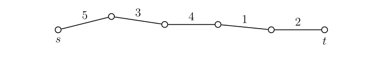
Remark. If the U −RT G is a path itself, then its maximum expected tem-poral distance is obviously n′.
s t
[image:12.612.112.489.373.448.2]5 3 4 1 2
Figure 3: MD of a U −RT G, which is a path itself, equals n′.
This can be easily understood if we consider that for any two vertices
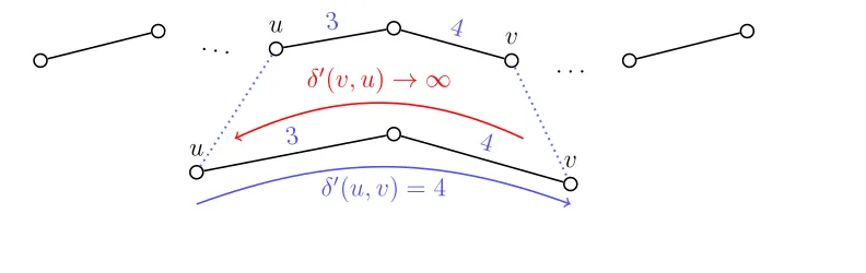
u and v in the path, if there exists a (u, v)-journey, then the time labels assigned to its edges form a strictly increasing sequence and thus there is no (v, u)-journey in it, apart from the slow journey which we assume that exists. Therefore, δ′(v, u) → +∞ and δ(v, u) = min{δ′(v, u), n′} = n′. (see
Figure 4).
4.1. Known graphs’ maximum expected temporal distance
u v
u 3 4 v
. . . 3 4
. . .
δ′(u, v) = 4
[image:13.612.125.521.138.263.2]δ′(v, u)→ ∞
Figure 4: Example of temporal distance, from source vertex to target vertex, equal to n′.
4.1.1. Case: G=Gstar
It is easy to understand that, even if the temporal star graph does not satisfy UNI-CASE, but satisfies any F-CASE, as defined in Section 2.1, it is:
maxs,t∈V(Gstar)EF δ(s, t)
≥2, for any distribution F
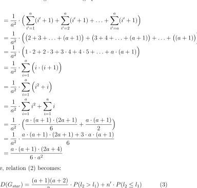
We will calculate the exact maximum expected temporal distance, MD, of a uniform random temporal star graph. It is:
MD(Gstar) =maxs,t∈V(Gstar)E δ(s, t)
=E δ(s, t), for any two vertices s, t∈V(Gstar)
=E(l2| l2 > l1)·P(l2 > l1) +n′·P(l2 ≤l1) (2)
We calculate the expected value of label l2, given that l2 > l1, that is
E(l2| l2 > l1):
E(l2| l2 > l1) =
a X
i=1
E(l2| l2 > i)·P(l1 =i)
= a X
i=1
Xa
i′=i
P(l2 =i′+ 1)·(i′ + 1)
·P(l1 =i)
= a X
i=1
Xa
i′=i
(i′ + 1)· 1
a
· 1a
= 1
a2 ·
a X
i=1
a X
i′=i
t
s
. . . l
2
[image:14.612.173.557.290.656.2]l1
Figure 5: A star graph
= 1
a2 ·
Xa
i′=1
(i′ + 1) + a X
i′=2
(i′+ 1) +. . .+ a X
i′=a
(i′+ 1)
= 1
a2 ·
2 + 3 +. . .+ (a+ 1)+ 3 + 4 +. . .+ (a+ 1)+. . .+ (a+ 1)
= 1
a2 ·
1·2 + 2·3 + 3·4 + 4·5 +. . .+a·(a+ 1)
= 1
a2 ·
a X
i=1
i·(i+ 1)
= 1
a2 ·
a X
i=1
i2 +i
= 1
a2 ·
a X
i=1
i2+
a X
i=1
i
= 1
a2 ·
a·(a+ 1)·(2a+ 1)
6 +
a·(a+ 1)
2
= 1
a2 ·
a·(a+ 1)·(2a+ 1) + 3·a·(a+ 1) 6
= a·(a+ 1)·(2a+ 4) 6·a2
Therefore, relation (2) becomes:
MD(Gstar) = (a+ 1)(a+ 2)
3a ·P(l2 > l1) +n
′·P(l
It holds that:
P(l2 ≤l1) =
a X
i=1
P(l2 ≤i)·P(l1 =i)
= a X
i=1
i
a ·
1
a
= 1
a2
a X
i=1
i
= a+ 1 2a
Therefore, it is:
P(l2 > l1) = 1−P(l2 ≤l1)
= a−1 2a
Relation (3) now becomes:
MD(Gstar) = (a+ 1)(a+ 2)
3a ·
a−1
2a +n
′ ·a+ 1
2a
Eventually, the star graph’s maximum temporal distance is:
MD(Gstar) = (a−1)(a+ 1)(a+ 2)
6a2 +n
′· a+ 1
2a
4.1.2. Case: G=Kn
We will now study extensively the clique’s case. First, let us observe that
δ′(s, t) ≤ a, and therefore δ(s, t) ≤ a, for any two vertices s, t in a clique.
Hence:
MD(Kn) =maxs,t∈V(Kn)E δ(s, t)
≤a
Normalized uniform random temporal clique. Let G = Kn be a clique of n vertices and let us consider its normalized U-version. That is, every edge
e ∈ E(Kn) is given a single availability label and those labels are chosen randomly and independently from one another from the setL0={1,2, . . . , n},
with the probability that an edge’s label equals i being equal to 1
n, ∀i∈L0. For any two vertices s, tin the clique, we have:
E l(e={s, t})= n
. . .
Figure 6: A clique
In the specific case of the normalized uniform random temporal clique of n vertices, there is actually no need for us to assume any slow journey to connect any pair of vertices since we already have such a journey, with arrival time equal to E l(e ={s, t}) = n
2. But, for the sake of consistency,
we can set the fixed number n′ to be equal to n
2.
It holds that:
MD(normalized Kn) =maxs,t∈V(Kn)E δ(s, t)
≤ n2
Since this is only an upper bound, we wonder if we can find temporal paths with smaller arrival time than that bound. Indeed, we give a simple (greedy)algorithm which can, with high probability, find a journey with small expected arrival time from a given source vertex s to a given target vertex t
in the normalized uniform random temporal clique.
Algorithm 1The normalized U-RTG clique short journey finding algorithm, Extend-Try
1: procedure Extend-Try(clique Kn, s, t, c1, k) 2: for i = 0 ... c1√nlogn do
3: si := undefined;
4: end for
5: s0 :=s;
6: for i = 0 ... c1√nlogn do
7: if l({si, t})∈ c1√n(logn)k, c1√n(logn)k+√n
then
8: Follow directly the edge {si, t}; Success!
9: go to line 20
10: else
11: if ∃u ∈ U \ {t} (where U stands for the set of the unvisited vertices) such, that l({si, u})∈ k·i, k(i+ 1)
then
12: si+1 =u;
13: go to line 6
14: else
15: follow directly the edge{si, u} with the smallest l({si, u}) among all u∈U; Failure!
16: go to line 23
17: end if
18: end if
19: end for
20: for i = 0 ... c1√nlogn do
21: return si; 22: end for
23: end procedure
Analysis of Extend-Try. Next, we analyze algorithm 1, looking for the prob-ability that it succeeds.
The probability that the time label of the edge {si, t} belongs to the interval (c1√nk, c1√nk+√n) and thus the algorithm succeeds in the (i+1)th
iteration, is:
Pl({si, t})∈ c1√n(logn)k, c1√n(logn)k+√n
=
√
n
n =
1
√
Let εj1 be the following event:
“The algorithm finds a proper journey s0s1, s1s2, s2, s3, . . . , sj−1sj”
meaning that it finds a temporal path, on the temporal edges of which we find strictly ascending time labels and in fact the ith temporal edge’s time label correctly belongs to the interval ((i−1)k, ik). The time labels are given to the edges independently from one another, thus the proba-bility that the event εj1 occurs is the product of the following probabili-ties: P∃s1 unvisited vertex : the edge {s0, s1} has time labell({s0, s1})∈
(0, k)
P∃s2 unvisited vertex : the edge {s1, s2} has time labell({s1, s2})∈(k,2k)
.. .
P∃sj unvisited vertex : the edge {sj−1, sj} has time label l({sj−1, sj}) ∈
(j−1)k, jk
For any ith probability of the above, it holds that:
P∃si unvisited vertex : the edge{si−1, si} has l({si−1, si})∈((i−1)k, ik)
= 1−P6 ∃si unvisited vertex : the edge {si−1, si} has l({si−1, si})∈ ((i−1)k, ik)
= 1−P∀si unvisited vertices : the edge {si−1, si} has l({si−1, si})∈/ ((i−1)k, ik)
= 1−P the edge {si−1, si} has l({si−1, si})∈/((i−1)k, ik), si unvisited vertex n−i
= 1−1−P the edge {si−1, si} has l({si−1, si})∈((i−1)k, ik), si unvisited vertex n−i
= 1−1− k
n
n−i
Therefore, the probability that εj1 occurs, is:
P(εj1) = 1−1− k
n
n−1!
·
1−1− k
n
n−2!
·. . .· 1−1− k
n
n−j!
≥ 1−1− k
n
n−j!j
≥
≥ 1−e−k1
− k
n
−j!j
Forj ≤c1√nlogn, we have:
1− k
n
−j
≤1− k
n
−c1√nlogn
⇔
⇔1−e−k1
− kn−j ≥1−e−k1
− kn−c1
√n
logn
and:
1−e−k1− k
n
−j!j
≥ 1−e−k1− k
n
−c1√nlogn
!c1√nlogn
As a result, for j ≤c1√nlogn, it is:
P(εj1)≥ 1−e−k1
− nk−c1
√nlogn!c1√nlogn
P(εj1)≥ 1−e−k1
− k
n
−c1√nlogn
It holds asymptotically:
c1√nlogn≤n ⇔
1− k
n
c1√nlogn
≥1− k
n
n
⇔
1− k
n
−c1√nlogn
≤1− k
n
−n
⇔
1−e−k1
− kn−c1
√nlogn
≥1−e−k1
− kn−n
Therefore:
P(εj1)≥1−e−k1
− nk−n
and since k ≥1, we have:
P(εj1)≥1−e−k
1− 1
n
= 1−e−ke = 1−e1−k
Fork =rlogn, r > 1, we have:
P(εj1)≥1−e1−rlogn
= 1−en−r
The probability that we fail in every iteration i = 0, . . . , c1√nlogn to
find a vertex si such, that l({si, t})∈(c1√nk, c1√nk+√n) is:
P(allf ail) =
c1√nlognfactors
z }| {
1− √1
n
·1− √1
n
·. . .1− √1
n
=1− √1
n
c1√nlogn
=e−c1logn =n−c1
The probability that we succeed in some iteration of the algorithm is:
P(success) =1−P(allf ail)P(εj1)
≥1−n−c1
1−en−r Therefore, the following theorem holds:
Theorem 1. For any constants c1, r > 1, given two vertices s, t, s 6= t, of the normalized uniform random temporal clique, Kn, the probability to arrive, starting from s, to t at time at most
t0 =c1√n(logn)k+√n, where k=rlogn
is at least
1−n−c1
1−en−r.
5. Temporal Diameter
In this section, we study the concept of the temporal diameter of a uniform random temporal graph.
Definition 6. Consider an instance G(L) of a U-RTG. We denote the max-imum of all distributional temporal distances between all pairs of vertices of
G(L) by d(G(L)):
d(G(L)) =maxs,t∈V(G)δ′(s, t).
We definediam(G(L)) =min{d(G(L)), n′}. Then, the Expected or Temporal
Diameter of G, denoted by T D, is given by the following formula:
T D(G) =Ediam G(L)=X
L
diam G(L)·P(L)
, where P(L) is the probability for labelling L to occur.
We can easily prove that every temporal graph’s temporal diameter,T D, is equal or greater than its maximum expected temporal distance, MD. Theorem 2. It holds that:
T D(G)≥MD(G), for every temporal graph G.
Proof. To prove this, we use the Reverse Fatou’s Lemma[D10]:
Theorem (Reverse Fatou’s lemma). If Xn≥0, for all n, then
E(limnsupXn)≥limnsupE(Xn).
In other words, the expected value of the maximum of a set of random variables is at least equal to the maximum of the expected values of those variables.
Now, notice that the Temporal Diameter of a temporal graphGis actually the expected value of the maximum of all distributional temporal distances, that isE(maxs,t∈V(G)δ′(s, t)), in the case where we haveδ′(s, t)≤n′, for every
Therefore, in that case, using the above described Reverse Fatou’s Lemma, we conclude that:
T D(G)≥MD(G).
In the case, where there is at least one pair of vertices s, t∈ V(G) such, that δ′(s, t) ≥ n′, both the temporal diameter and the maximum expected
temporal distance of G are equal to n′.
Thus, we conclude that it generally applies that:
T D(G)≥MD(G), for every temporal graphG.
We will now prove that the timet0−o(t0) (see. Theorem 1) is an upper
bound of the normalized uniform random temporal clique’s temporal diam-eter, T D, and, thus, is an upper bound of its maximum expected temporal distance, MD.
Theorem 3. The quantity t0−o(t0) is an upper bound of both the temporal diameter, T D, and the maximum expected temporal distance, MD, of the normalized U-RT clique.
Proof. Let s, t be two vertices of the normalized U-RT clique. We call Est the following event:
“We arrive, starting from s, to t at time at most to”
where t0 =c1√n(logn)k+√n, c1 >1, k=rlogn, r >1.
It holds that:
P(Est)≥1−n−c1
1−en−r
≥1−n−c1 −en−r
Forr=c1, the above relation becomes:
P(Est)≥1−n−c1 −en−c1
Therefore, the probability that the complement ofEst occurs is:
P(Est) = 1−P(Est)
≤2en−c1
Thus, the probability that there exist two verticess, tsuch that we arrive, starting from s, to t at time greater than t0 is:
P(∃s, t:Est)≤n(n−1)2en−c1
≤2en−c1−2
Let us denote by T the max{ast, s, t ∈V(Kn)}, where ast is the greatest arrival time amongst all (s, t)-journeys’ arrival times. Then, we have:
P(∃s, t:Est) =P(T > t0)
≤2en−c1−2
It is:
T D ≤E(max{ast, s, t ∈V(Kn)})
≤(1−2en−c1−2)·t
0+n·2en−c1−2
≤t0−o(t0)
Since T D(G)≥ MD(G), for every temporal graph G, we conclude that in the case of the normalized U-RT clique, it is:
MD ≤T D ≤t0−o(t0)
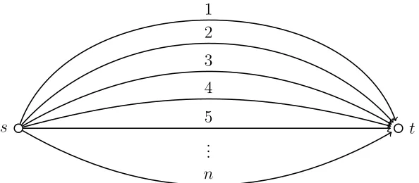
6. An optimization problem: The Bridges’ problem
We will now study an optimization problem concerning the temporal multigraph shown in Figure 7.
The problem
s t
1 2 3 4 5 ...
[image:24.612.158.455.149.279.2]n
Figure 7: The bridges’ problem
of a total ofn bridges that connect the two riversides, paying individual cost equal to 1 + i
mi
, wherei stands for the number of the bridge they pass and
mi stands for the total sum of people that cross that bridge. Thus, the total cost payed by m people to cross the ith bridge,i= 1,2, . . . , n, is:
cost[i] =mi+i
We denote by maximum cost payed the maximum, over all bridges i, cost
mi+i:
maximum cost payed=max{mi+i, i= 1,2, . . . , n: bridge}
How should the n people be assigned to the bridges so, that the maximum cost payed is minimized?
We denote the minimum, over all assignments of n people to n bridges, maximum cost payed by OP T, that is:
OP T =minall assignments{maximum cost payed}
s 1,2, . . . , n t
Figure 8: The bridges’ problem (another interpretation)
Here we have a single bridge which is available everyday from day 1 to day
n. As time progresses the cost someone needs to pay to move from s to t
increases. Again, one has to pay individual cost equal to 1 + i
mi
, where i
stands for the day on which he decides to move from s to t and mi stands for the total sum of people decide to move from s tot on that same day. Therefore, the total cost payed bym people who move from s tot on theith
day, i= 1,2, . . . , n, is:
cost[i] =mi+i
Theorem 4. We can compute the assignment of n persons to n bridges that achieves the OP T in polynomial time O(n2).
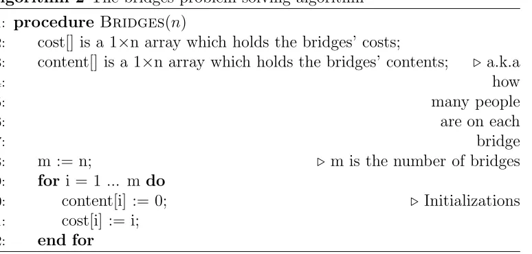
Proof. We provide Algorithm 2 and show that it computes the assignment that achieves OP T.
Algorithm 2 The bridges problem solving algorithm
1: procedure Bridges(n)
2: cost[] is a 1×n array which holds the bridges’ costs;
3: content[] is a 1×n array which holds the bridges’ contents; ⊲a.k.a
4: how
5: many people
6: are on each
7: bridge
8: m := n; ⊲ m is the number of bridges
9: for i = 1 ... m do
10: content[i] := 0; ⊲ Initializations
11: cost[i] := i;
Algorithm 2 The bridges problem solving algorithm (continued)
13: for i = 1 ... n do
14: bridge := 1; ⊲ Initialize the bridge that the ith person will pass
15: for j = 2 ... m do ⊲ Find the bridge that gives the minimum
16: possible cost
17: if cost[j] <cost[bridge] then
18: bridge := j;
19: end if
20: end for
21: content[bridge] := content[bridge]+1; ⊲ Add the ith person to
22: the selected
23: bridge’s content
24: cost[bridge] := cost[bridge]+1; ⊲ Calculate the right new cost 25: end for
26: for i = 1 ... m do
27: if content[i] == 0 then 28: cost[i] := 0;
29: end if
30: if content[i] == 1 then
31: Write content[i] , “ person passes bridge #”, i , “ who therefore has to pay cost equal to ”, cost[i];
32: else
33: Write content[i] , “ people pass bridge #”, i , “ who therefore have to pay cost equal to ”, cost[i];
34: end if ⊲ Print the bridges’ costs
35: end for
36: end procedure
The algorithm assigns theith person to the bridge, for which the current minimum cost is payed. If there are more than one such bridges, the algo-rithm assigns the ith person to the first one in order. It is trivial to see that the algorithm’s running time is O(n2).
Proof of correctness We will prove the validity of the algorithm 2 by induction on the number n of persons.
the sole person is assigned to the bridge, paying cost equal to:
cost[1] = 2
So, actually, the algorithm solves the problem for n = 1 person.
• Assume that the algorithm solves the problem for n=k people.
• We will show that the algorithm solves the problem for n = k + 1 people.
Before continuing, let us consider the following: Letn1, n2 ∈Nnumbers
of people, with n1 > n2. It is obvious that the minimum possible
maximum cost for n = n1 people is at least equal to the minimum
possible maximum cost for n =n2 people.
Let us observe now that the procedures performed by the algorithm in the main loop for k people, and the results obtained through these, are identical to those performed and obtained respectively for k+ 1 people, except that for k+ 1 people, there is a (k+ 1)th bridge, which throughout the execution of these processes has zero content, and there is also an additional execution of the loop. At the beginning of this (k+ 1)th execution, the algorithm has already assigned the k people to the brisges in a way that we obtain the minimum possible maximum cost.
The algorithm, by construction, assigns the people to the bridges in a way that their costs are ordered by (not necessarily strictly) descending order and indeed one of the following two possible events occur:
all the bridges have the same cost, denoted byOP T
or
some bridges have cost OP T and some others have cost OP T −1.
In the second case, the algorithm is obviously going to assign the (k+ 1)th person to the first in order bridge that has cost equal toOP T
−1, thereby maintaining the maximum cost that occurs on the bridges to a minimum, that is OP T.
r+content[r] =OP T
But: content[r]≥1 and so: r+content[r]≥r+ 1
⇒OP T ≥r+1
Also, since the(r+ 1)th bridge has zero content, it is:
cost[r+ 1] =r+ 1
The algorithm checks which of thek+ 1 bridges has the minimum cost to assign the (k + 1)th person to that bridge. If OP T = r + 1, then the algorithm assigns the last person to the 1st bridge. Otherwise, it assigns it to the (r+ 1)th bridge. This way, it ensures the minimum possible maximum cost for the k+ 1 bridges.
Therefore, the algorithm solves the problem for n =k+ 1 people.
We will now calculate the value of the OP T. Again, let us denote by r
the number of bridges that have a positive content, i.e. are not empty, in the optimal case which the Algorithm 2 computes. For the sake of brevity, let us also denote by li the content of the ith bridge. Since the average cost of the non empty bridges is equal or less than the maximum cost that occurs on those bridges, the following holds for the optimal case:
r X
i=1
(i+li)
r ≤OP T
Therefore, we have:
r X
i=1
(i+li)≤rOP T (4)
Furthermore, it is easy to see that since, in the optimal case that the algorithm computes, the OP T is greater than any bridge’s cost by at most one, it holds that:
rOP T −r ≤
r X
i=1
By the relations (4) and (5), we have:
rOP T−r ≤
r X
i=1
(i+li) ≤rOP T⇔
rOP T−r ≤
r X
i=1
i+
r X
i=1
li ≤rOP T⇔
rOP T−r ≤ r(r+ 1)
2 +n ≤rOP T⇔
OP T −1 ≤ (r+ 1)
2 +
n
r ≤OP T
Now, the quantity (r+1)2 + n
r is minimized at r=
√
2n and at that point, its value is equal to √2n+1
2. Therefore, we conclude that:
OP T =⌈√2n+1
2⌉
7. Conclusions and further research
References
[MMCS13] George Mertzios, Othon Michail, Ioannis Chatzigiannakis, and Paul G. Spirakis (2013).Temporal Network Optimization Subject to Con-nectivity ConstraintsSpringer
[KKK00] D. Kempe, J. Kleinberg, and A. Kumar (2000). Connectivity and inference problems for temporal networksIn Proceedings of the 32nd an-nual ACM symposium on Theory of computing (STOC)
[MR02] M. Molloy and B. Reed (2002).Graph colouring and the probabilistic method, volume 23 Springer