arXiv:1703.02776v1 [math.AG] 8 Mar 2017
TOM BRIDGELAND
Abstract. We study the Riemann-Hilbert problems associated to the Donaldson-Thomas theory
of the resolved conifold. We give explicit solutions in terms of the Barnes double and triple sine functions. We show that the correspondingτ-function is a non-perturbative partition function, in the sense that its asymptotic expansion coincides with the topological string partition function.
1. Introduction
In [6] we studied a class of Riemann-Hilbert problems arising naturally in Donaldson-Thomas theory. They involve piecewise holomorphic maps from the complex plane into an algebraic torus (C∗)n with prescribed discontinuities along a given collection of rays. These problems represent
the conformal limit of the Riemann-Hilbert problems appearing in the work of Gaiotto, Moore and Neitzke [12]. The purpose of this paper is to give a detailed solution to the Riemann-Hilbert problems associated to the resolved conifold using a class of special functions related to Barnes’ multiple gamma functions [1, 2, 3]. We also compute the τ-function in the sense of [6], and show that the asymptotic expansion of log(τ) reproduces the positive degree terms in the genus expansion of the topological string free energy. Our calculations thus suggest a new approach to defining non-perturbative partition functions in topological string theory.
1.1. BPS structures for the resolved conifold. Let X denote the resolved conifold: this is the non-compact Calabi-Yau threefold which is the total space of the vector bundle OP1(−1)⊕2.
Contracting the zero-section C ⊂X gives the threefold ordinary double point x1x2 −x3x4 ⊂C4.
The Riemann-Hilbert problems we shall consider arise from the Donaldson-Thomas (DT) theory of the category of compactly-supported coherent sheaves on X. They depend on a point in the space
M =
(v, w)∈C2 :w6= 0 and v+nw 6= 0 for all n∈Z ⊂C2.
Mathematically speaking, as we recall in Appendix A, this is the space of stability conditions on the derived category DbCoh(X), quotiented by the subgroup of the group of auto-equivalences
generated by spherical twists. From the physical standpoint, it can be thought of as the smallest unramified cover of the natural C∗-bundle over the stringy K¨ahler moduli space on which central charges of branes are single-valued.
Associated to a point ofM is a collection of data which we referred to in [6] as a BPS structure. Mathematically it represents the output of unrefined DT theory applied to the given stability
condition. In physical terms it encodes the BPS invariants of the non-linear supersymmetric sigma model associated to the space X. It consists of
(i) The charge lattice Γ≤1 =Zβ⊕Zδ equipped with the skew-symmetric formh−,−i= 0.
(ii) The central charge: this is the group homomorphism
Z≤1: Γ≤1 →C, Z≤1(aβ+bδ) = 2πi(av+bw).
(iii) The nonzero BPS invariants
Ω(γ) =
1 if γ =±β+nδ for some n∈Z,
−2 if γ =kδ for some k ∈Z\ {0}. (1)
.
The lattice Γ≤1 is the natural receptacle for Chern characters of compactly-supported sheaves
onX. All such sheaves are supported in dimension≤1: the most important examples are the line bundles OC(n) supported on the zero-sectionC ⊂X, and the skyscraper sheaves Ox supported at
points x∈X. We have
ch(OC(n)) = β+nδ, ch(Ox) =δ.
The two cases in (1) give the contribution to DT theory from sheaves supported in dimension one and zero respectively, and arise from the above-mentioned sheaves and their shifts. For the mathematical derivation of (1) we refer to [16, Example 6.30].
The form h−,−i, which in the general context of [6] is the Euler form of the relevant category, vanishes in this case because curves on a threefold have zero intersection number. This has the consequence that the BPS invariants Ω(γ) do not depend on the choice of point (z, w)∈M. It also implies that the Riemann-Hilbert problem associated to our BPS structure is trivial. To remedy this we consider the double of the above BPS structure. This involves replacing the lattice Γ≤1
with the lattice
Γ = Γ≤1⊕Γ≥2, Γ≥2 := Γ∨≤1 = HomZ(Γ≤1,Z),
equipped with the canonical non-degenerate integral skew-symmetric form, and extending the map Ω by zero. We can extend the map Z≤1 via an arbitrary group homomorphism
Z≥2: Γ≥2 →C,
so that the space of possible doubled BPS structures becomes the cotangent bundle T∗M.
1.2. The Riemann-Hilbert problem. Introduce the twisted torus
T=
g: Γ→C∗ :g(γ1+γ2) = (−1)hγ1,γ2ig(γ1)·g(γ2) .
It is a torsor for the algebraic torus HomZ(Γ,C∗), and hence non-canonically isomorphic to (C∗)4.
For each class γ ∈Γ there is a twisted character
The ray diagram associated to a BPS structure consists of the raysR>0·Z(γ) determined by those classes γ ∈Γ for which Ω(γ)6= 0. These rays are said to be active. The ray diagram for the BPS structure corresponding to a point (v, w) ∈ M+ is illustrated in Figure 1 below. Note that the
doubling procedure does not affect this.
The Riemann-Hilbert problem associated to the doubled BPS structure defined by a point of
T∗M depends also on the choice of an element ξ ∈T called the constant term. The problem then asks for a piecewise holomorphic map Φ : C∗ →Twhich is holomorphic in the complement of the active rays, has a prescribed discontinuity as t∈C∗ crosses an active ray ℓ⊂C∗, and has certain given limiting behaviour as t→0 or t→ ∞. Composing with the twisted characters of T we can equivalently encode the solution in the system of maps
Φγ: C∗ →C∗, Φγ(t) =xγ(Φ(t))
parameterised by γ ∈Γ.
In a bit more detail, the required discontinuity ast ∈C∗ crosses an active ray ℓ⊂C∗ is
Φβ(t)7→Φβ(t)·
Y
Z(γ)∈ℓ
(1−Φγ(t))Ω(γ)hβ,γi,
and we ask that
exp(Z(γ)/t)·Φγ(t)→xγ(ξ),
as t → 0, and that each Φγ(t) should have moderate growth as t → ∞, in the sense that there
exists k >0 such that for all|t| ≫0
|t|−k <|Φγ(t)|<|t|k.
We review the precise details of the Riemann-Hilbert problem in Sections 2 and 3. Our first main result can be summarised in the following form.
Theorem 1.1. Consider the doubled BPS structure corresponding to a point of T∗M, and choose a constant term ξ ∈ T which satisfies xγ(ξ) = 1 for all classes γ ∈ Γ≤1. Then the corresponding
Riemann-Hilbert problem has a unique solution, which can be written explicitly in terms of Barnes
double and triple sine functions.
We will give a more precise statement of this result in Section 5, after the relevant special functions have been introduced in Section 4.
1.3. The τ-function. It turns out that the unique solution to the Riemann-Hilbert problems for all points (v, w) ∈ M, and fixed constant term ξ ∈ T, can be encoded in a single piecewise-holomorphic functionτ =τ(v, w, t). To do this we first re-express the unique solutions of Theorem 1.1 in terms of maps Ψγ: C∗ →C∗ by writing
It is easy to see that the maps Ψγ are independent of the extended part of the central charge Z≥2, and therefore only depend on v, w and t. We then look for a piecewise-holomorphic function
τ =τ(v, w, t) which is invariant under simultaneous rescaling of all variables, and which satisfies
∂
∂tlog Ψβ∨(t) = ∂
∂vlogτ(v, w, t),
∂
∂tlog Ψδ∨(t) = ∂
∂wlogτ(v, w, t).
When it exists, such a function τ is easily seen to be unique up to multiplication by a nonzero constant. We review the details of this definition in Section 2.
In the case of the Riemann-Hilbert problems associated to the resolved conifold we show that a
τ-function in the above sense does indeed exist, and we compute it explicitly. Let us introduce a function H(v, w, t) via the integral representation
H(v, w, t) = exp
Z
C
evs−1 ews −1·
ets
(ets−1)2 ·
ds s
!
, (2)
where the contour C is the real axis with a small detour above the origin. This representation is valid for 0≤Re(v)≤Re(w). Let us also introduce
R(v, w, t) = w 2πit
2
Li3(e2πiv/w)−ζ(3)
+ iπ 12·
v w.
In Section 5 we shall prove
Theorem 1.2. The expression
τ(v, w, t) =H(v, w, t)·exp(R(v, w, t))
defines a τ-function for the variation of BPS structures defined by the resolved conifold. As t→0
there is an asymptotic expansion
logτ(v, w, t) ∼ − 1
12log
w
t
+ iπ 12·
v w+
X
g≥1
B2g ·Li3−2g(e2πiv/w)
2g·(2g−2)!
2πit w
2g−2
+X
g≥2
B2g·B2g−2
2g·(2g−2)·(2g−2)!
2πit w
2g−2
.
1.4. Some motivation from mirror symmetry. Classical mirror symmetry [8, 13] relates the periods of a Calabi-Yau threefoldY to generating functions for enumerative invariants of a mirror Calabi-Yau threefold X. This can be viewed as an identification between two variations of Hodge structures (VHS). On one side is the classical VHS on the moduli space of complex structures on Y, considered in a neighbourhood of a maximally unipotent degeneration. On the other is a VHS over the complexified K¨aher cone ofX, constructed from the genus 0 Gromov-Witten (GW) invariants of X.
There is an obvious asymmetry here, in that the moduli of complex structures on Y is a global space with interesting topology, which we are choosing to view near a given boundary point, whereas on the other side, the complexified K¨aher cone of X has no interesting topology. To remove this, we would like to see the complexified K¨ahler cone as a neighbourhood of a boundary point in a larger space with non-trivial topology. Moreover one would like to be able to extend the VHS on the K¨ahler cone to a global VHS on this ‘stringy’ K¨ahler moduli space. Mirror symmetry should then give rise to a map between the complex moduli space of X and the stringy K¨ahler moduli space of Y, identifying the two VHS.
Our best hope for a mathematical definition of such a stringy K¨ahler moduli space is via the space of stability conditions [4,9] on the derived category of coherent sheaves D(X) =DbCoh(X).
In fact this space Stab(X) is better thought of as being mirror to the space of deformations of the category D(Y), which contains the classical moduli space of complex structures on Y within it (see [5, Section 7]). On this larger space one should expect a generalization of the concept of a VHS referred to in [18] as a non-commutative VHS. Nonetheless, the general conclusion remains that one should seek a geometric structure on the space of stability conditions which reproduces the A-model VHS in the large volume limit.
The definition of the GW invariants ofX is too geometric in nature to generalise to the derived category D(X). Instead, the natural enumerative invariants associated to points of the space Stab(X) are (generalized) DT invariants [16,19], which encode the virtual Euler characteristics of moduli spaces of stable objects of each given Chern character. Although rank 1 DT invariants are known to encode equivalent data to the GW invariants [23,27], the two systems of invariants have very different formal properties. In particular, it is not at all clear how to extract a VHS from DT theory: in the case of GW theory this arises from the geometric properties of the compactification of the moduli of stable maps.
We view the calculations of this paper as an indication that this approach is on the right lines. We are performing a natural construction on the space of stability stability conditions which is appropriately invariant under the group of autoequivalences, and are obtaining non-perturbative quantities which reproduce Gromov-Witten theory near the large volume limit.
Acknowledgements. I thank Alba Grassi, Kohei Iwaki and Bal´azs Szendr˝oi for useful remarks. I am particularly grateful to Simon Ruijsenaars for his expert help with multiple sine functions.
2. BPS structures and Riemann-Hilbert problems
In this section we recall some relevant definitions and results from [6].
2.1. BPS structures and their doubles. We start with the basic definition
Definition 2.1. A BPS structure (Γ, Z,Ω) consists of
(a) A finite-rank free abelian group Γ∼=Z⊕n, equipped with a skew-symmetric form
h−,−i: Γ×Γ→Z,
(b) A homomorphism of abelian groupsZ: Γ→C,
(c) A map of sets Ω : Γ→Q,
satisfying the following properties:
(i) Symmetry: Ω(−γ) = Ω(γ) for all γ ∈Γ,
(ii) Support property: fixing a norm k · kon the finite-dimensional vector space Γ⊗ZR, there
is a constant C >0 such that
Ω(γ)6= 0 =⇒ |Z(γ)|> C· kγk. (3)
The group homomorphism Z is called the central charge. The rational numbers Ω(γ) are called BPS invariants. A class γ ∈Γ is called active if Ω(γ)6= 0. We call a BPS structure (Z,Γ,Ω)
(i) convergent, if for someR >0
X
γ∈Γ
|Ω(γ)| ·e−R|Z(γ)|<∞, (4)
(ii) uncoupled, if for any two active classes γ1, γ2 ∈Γ one has hγ1, γ2i= 0.
Given a BPS structure (Γ, Z,Ω) the doubled BPS structure takes the form
(Γ⊕Γ∨, Z⊕Z∨,Ω),
where Γ∨ = Hom
Z(Γ,Z) is the dual lattice, andZ∨: Γ∨ →Cis an arbitrary group homomorphism.
We equip the doubled lattice ΓD = Γ⊕Γ∨ with the non-degenerate skew-symmetric form
(γ1, λ1),(γ2, λ2)
The central charge is defined by Z(γ, λ) =Z(γ), and the BPS invariant Ω(γ, λ) is defined to be zero unless λ= 0 in which case Ω(γ,0) = Ω(γ).
2.2. Twisted torus. Given a BPS structure (Γ, Z,Ω), we consider the algebraic torus
T+= HomZ(Γ,C∗)∼= (C∗)n
and its co-ordinate ring (which is also the group ring of the lattice Γ)
C[T+] =C[Γ]∼=C[y±11,· · · , y±nn].
We write yγ ∈ C[T+] for the character of T+ corresponding to an element γ ∈ Γ. The
skew-symmetric form h−,−iinduces an invariant Poisson structure on T+, given on characters by
{yα, yβ}=hα, βi ·yα·yβ. (6)
The twisted torus of the BPS structure is a torsor over T+ defined by
T=T−={g: Γ→C∗ :g(γ1+γ2) = (−1)hγ1,γ2ig(γ1)·g(γ2)},
The co-ordinate ring of T− is spanned as a vector space by the twisted characters xγ: T− → C∗ tautologically defined by xγ(g) =g(γ)∈C∗. Thus
C[T−] =M
γ∈Γ
C·xγ, xγ1 ·xγ2 = (−1)hγ1,γ2i·xγ1+γ2. (7)
There is a Poisson bracket on C[T−] given on twisted characters by
{xα, xβ}=hα, βi ·xα·xβ. (8)
A ray ℓ = R>0·z ⊂ C∗ is called active if it contains a point Z(γ) for some active class γ ∈ Γ. Associated to any ray ℓ⊂C∗ is a formal sum of twisted characters
DT(ℓ) = X
γ∈Γ:Z(γ)∈ℓ
DT(γ)·xγ. (9)
We would like to define an associated automorphism S(ℓ) of the twisted torusTby taking the time 1 Hamiltonian flow of this function. In fact the best we can hope for in general is a partially-defined automorphism, as explained in the next subsection.
2.3. BPS automorphisms. Let (Γ, Z,Ω) be a convergent BPS structure and fix an acute sector ∆⊂C∗. For each real number R > 0 we define U∆(R)⊂T to be the interior of the subset
g ∈T:Z(γ)∈∆ and Ω(γ)6= 0 =⇒ |g(γ)|<exp(−Rkγk) ⊂T.
It is proved in [6, Appendix B] that this is a non-empty open subset. The height of an active ray
ℓ⊂C∗ is defined to be
H(ℓ) = inf
Non-active rays are considered to have infinite height. The support property ensures that for any
H >0 there are only finitely many rays of height < H. The following statement can be found in [6, Section 4] and is proved in [6, Appendix B].
Proposition 2.2. For sufficiently large R >0 the following statements hold:
(i) For each ray ℓ⊂∆, the power series DT(ℓ) is absolutely convergent on U∆(R), and hence
defines a holomorphic function
DT(ℓ) : U∆(R)→C.
(ii) The time 1 Hamiltonian flow of the function DT(ℓ) with respect to the Poisson structure
{−,−} on T defines a holomorphic embedding
S(ℓ) :U∆(R)→T.
(iii) For each H >0, the composition in clockwise order
S<H(∆) =Sℓ1 ◦Sℓ2 ◦ · · · ◦Sℓk,
corresponding to the finitely many raysℓi ⊂∆of height < H exists, and the pointwise limit
S(∆) = lim
H→∞S<H(∆) : U∆(R)→T is a well-defined holomorphic embedding.
We think of the maps S(ℓ) constructed in Proposition 2.2 as giving partially-defined automor-phisms of the twisted torus T. The following result is proved in [6, Appendix B].
Proposition 2.3. Fix a ray ℓ⊂C∗ and suppose that the following conditions are satisfied: (i) there are only finitely many active classes γi ∈Γ with Z(γ)∈ℓ.
(ii) any two active classes γi ∈Γ with Z(γi)∈ℓ satisfy hγi, γji= 0,
(iii) any active class γ ∈Γ with Z(γ)∈ℓ has Ω(γ)∈Z.
Then the map S(ℓ) of Proposition 2.2 extends to a birational automorphism of T whose pullback
on twisted characters is given by
S(ℓ)∗(x
β) = xβ·
Y
Z(γ)∈ℓ
(1−xγ)Ω(γ)hβ,γi. (10)
2.4. Riemann-Hilbert problem. Let (Γ, Z,Ω) be a convergent BPS structure. Given a ray
ℓ⊂C∗ we consider the corresponding half-plane
Hℓ =ℓ·h={z ∈C∗ :z=u·v with u∈ℓ and Re(v)>0},
centered on it. We shall be dealing with functions of the form Φℓ: Hℓ →T. Composing with the
twisted characters of Twe can equivalently consider functions
The Riemann-Hilbert problem associated to the BPS structure (Γ, Z,Ω) depends on a choice of element ξ∈T which we refer to as the constant term.
Problem 2.4. Fix an element ξ ∈ T. For each non-active ray ℓ ⊂ C∗ we seek a holomorphic function Φℓ: Hℓ →T such that the following three conditions are satisfied:
(RH1) Jumping. Suppose that two non-active raysℓ1, ℓ2 ⊂C∗ form the boundary rays of a convex
sector ∆⊂C∗ taken in clockwise order. Then
Φℓ1(t) =S(∆)◦Φℓ2(t),
for all t∈Hℓ1 ∩Hℓ2 with 0<|t| ≪1.
(RH2) Finite limit at 0. For each non-active ray ℓ⊂C∗ and each classγ ∈Γ we have
exp(Z(γ)/t)·Φℓ,γ(t)→ξ(γ)
as t→0 in the half-plane Hℓ.
(RH3) Polynomial growth at ∞. For any class γ ∈Γ and any non-active ray ℓ ⊂C∗, there exists
k >0 such that
|t|−k<|Φℓ,γ(t)|<|t|k,
for t∈Hℓ satisfying |t| ≫0.
To make sense of the condition (RH1) note that condition (RH2) implies that Φℓi(t) ∈U∆(R)
whenever t ∈Hℓ1 ∩Hℓ2 with 0 <|t| ≪ 1. But we can find R >0 such that the partially-defined
automorphism S(∆) is well-defined on the open subset U∆(R)⊂ T. Thus the given relation does
indeed make sense.
It will be useful to consider the maps Ψℓ: Hℓ →T+ defined by
exp(Z/t)·Φℓ(t) = Ψℓ(t)·ξ.
Composing with the characters of T+ we can also encode the solution in the system of maps
Ψℓ,γ(t) =xγ(Ψℓ(t)) = exp(Z(γ)/t)·Φℓ,γ(t)·ξ(γ)−1.
Of course the maps Φℓ and Ψℓ are equivalent data: we use whichever is most convenient.
An element γ ∈Γ will be called null if it satisfies hα, γi= 0 for all active classes α ∈ Γ. Note that the definition of the wall-crossing automorphisms S(ℓ) then implies thatS(ℓ)∗(x
γ) =xγ. The
following result is proved in [6, Section 4.5].
Proposition 2.5. Let (Γ, Z,Ω) be a convergent BPS structure, and fix a constant term ξ ∈T. (i) If a classγ ∈Γ is null then any solution to Problem2.4 satisfies Ψℓ,γ(t) = 1 for all t ∈Hℓ.
2.5. The τ-function. A variation of BPS structures (Γp, Zp,Ωp) over a complex manifold M
consists of a family of BPS structures indexed by the pointsp∈M satisfying certain axioms, the most important of which is the Kontsevich-Soibelman wall-crossing formula, which describes the way the BPS invariants Ωp(γ) change as the point p ∈ M moves. A complete definition is given
in [6, Appendix A].
For the purposes of this paper however, it is sufficient to consider the much simpler notion of a framed variations of uncoupled BPS structures over a complex manifoldM, which is nothing more than a family of BPS structures (Γ, Zp,Ω) indexed by the pointsp ∈ M, such that the lattice Γ, the form h−,−i, and the BPS invariants Ω(γ) are all constant, and such that for any γ ∈Γ, the central charge Zp(γ)∈C varies holomorphically.
Given a variation of BPS structures, the obvious map
π: M →HomZ(Γ,C)∼=Cn, p7→Zp
is called the period map, and the variation is called miniversal if it is a local isomorphism. In that case, if we choose a basis (γ1,· · · , γn) ⊂ Γ, the functions zi = Z(γi) form a system of local
co-ordinates near any given point of M.
For each point p ∈ M we can consider the Riemann-Hilbert problem associated to the BPS structure (Γ, Zp,Ω) and seek a family of solutions given by a piecewise-holomorphic map
Ψ :M ×C∗ →T+,
which we view as a function of the co-ordinates (z1,· · · , zn) ∈Cn and the parameter t ∈C∗. We
define aτ-function for this family of solutions to be a piecewise-holomorphic map
τ: M ×C∗ →C∗,
which is invariant under simultaneous rescaling of all co-ordinates zi and the parameter t, and which satisfies the equations
∂log Ψγi ∂t =
X
j
hγi, γji∂logτ
∂zj . (11)
When the formh−,−iis non-degenerate these conditions determineτ uniquely up to multiplication by a constant scalar factor. The author does not yet have a good explanation of why such a function τ should exist in general, but in the case of the variation of BPS structures associated to the resolved conifold, such a function can indeed be defined.
3. The conifold Riemann-Hilbert problem
3.1. The BPS structures. The BPS structures we shall consider depend on a point in the space
M =
(v, w)∈C2 :w6= 0 and v+nw 6= 0 for all n∈Z ⊂C2.
Mathematically speaking, as we recall in Appendix A, this is the space of stability conditions on the derived category of the resolved conifold, quotiented by the subgroup of the autoequivalence group generated by spherical twists. From the physical standpoint it can be thought of as the smallest unramified cover of the naturalC∗-bundle over the stringy K¨ahler moduli space on which the central charges of branes are single-valued. We decompose
M =M+⊔M0⊔M−
according to the sign of Im(v/w). The BPS structure (Γ≤1, Z≤1,Ω) corresponding to a point
(v, w)∈M is given by
(i) The lattice Γ≤1 =Zβ⊕Zδ with the form h−,−i= 0.
(ii) The central charge Z≤1: Γ≤1 →Cdefined by
Z≤1(aβ+bδ) = 2πi(av+bw).
(iii) The non-zero BPS invariants
Ω(γ) =
1 if γ =±β+nδ with n ∈Z,
−2 ifγ =nδ with n∈Z\ {0}.
(12)
Together these structures form a framed and miniversal variation of uncoupled BPS structures over M. The BPS invariants are constant becauseh−,−i= 0. We also consider the corresponding doubled BPS structures. As in the introduction we denote these by (Γ, Z,Ω) and use the notation
Γ = Γ≤1⊕Γ≥2, Γ≥2 := Γ≤∨1 = HomZ(Γ≤1,Z).
We denote by (β∨, δ∨)⊂Γ≥
2 the dual basis to (β, δ)⊂Γ≤1. The map Ω : Γ→Qsatisfies Ω(γ) = 0
unless γ ∈Γ≤1. The central charge takes the form
Z =Z≤1⊕Z≥2: Γ→C,
where the group homomorphism Z≥2: Γ≥2 →C is arbitrary. The resulting BPS structures are all
convergent, because
X
γ∈Γ
|Ω(γ)| ·e−|Z(γ)| = 2X
n∈Z
e−|v+nw|+ 2X
n≥0
e−n|w|<∞.
· · · · · ·
· · · · · ·
ℓ0
ℓ−1 ℓ1
−ℓ∞ ℓ∞
−ℓ0
−ℓ−1 −ℓ1
Σ(0) Σ(1)
2πiw
[image:12.612.131.481.57.302.2]2πiv
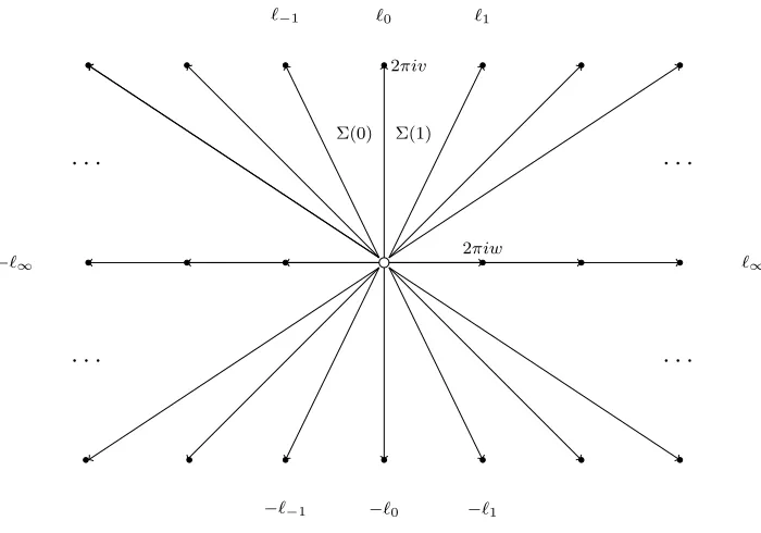
Figure 1. The ray diagram associated to a point (v, w)∈M+.
3.2. BPS automorphisms. Let us fix a point (v, w)∈M+. Define rays
ℓ∞=R>0·2πiw, ℓn =R>0 ·2πi(v+nw)⊂C∗.
The active rays for the corresponding BPS structure (Γ, Z,Ω) defined above are precisely the rays
±ℓ∞ and ±ℓn forn∈Z. The corresponding ray diagram is illustrated in Figure1. We let Σ(n) be the convex open sector with boundary raysℓn−1 andℓn. Note that the union of the active rays is a
closed subset of C∗ whose open complement is the disjoint union of the open sectors ±Σ(n)⊂C∗. We shall now describe explicitly the BPS automorphismsS(ℓ) of the twisted torusTassociated to the doubled lattice Γ = Γ≤1⊕Γ≥2. We denote byxγ: T→C∗ the twisted character corresponding
to an element γ ∈ Γ. Since, all active classes lie in Γ≤1 ⊂Γ, and the form h−,−i is zero on Γ≤1,
it follows that all classes γ ∈ Γ≤1 are null, and hence all BPS automorphisms act trivially on the
corresponding twisted characters xγ.
Proposition2.3 shows that the BPS automorphism associated to the rayℓn takes the form
S(ℓn)∗(xγ) =xγ·(1−xβ+nδ)hγ,β+nδi.
In particular, the twisted characters for the generators (β∨, δ∨)⊂Γ≥
2 transform as
S(ℓn)∗(xβ∨) =xβ∨ ·(1−xβ+nδ), S(ℓn)∗(xδ∨) =xδ∨ ·(1−xβ+nδ)n. (13)
characters is given by
S(ℓ∞)∗(xγ) =xγ·Y k≥1
(1−xkδ)−2k·hγ,δi.
It then follows that S(ℓ) extends to the analytic open subset of T where |xδ| < 1, but not to a Zariski open subset. The action on the basic twisted characters as above is
S(ℓ∞)∗(xβ∨) =xβ∨, S(ℓ∞)∗(xδ∨) = xδ∨ ·
Y
k≥1
(1−xkδ)−2k.
Remark 3.1. There is no need to consider the active rays −ℓn and −ℓ∞ separately, since as explained in [6, Section 4.4], for any rayℓ ⊂C∗ there is a relation
S(−ℓ)◦σ =σ◦S(ℓ), (14)
where σ: T→T is the involution which acts on twisted characters as xγ ↔x−γ.
We shall also need to describe the BPS automorphisms S(∆) associated to convex sectors ∆⊂ C∗. There are two possibilities: either ∆ contains a finite number of active rays, or it contains
one of the two rays ±ℓ∞, and hence also an infinite number of the rays ±ℓn. In the first case the corresponding BPS automorphism S(∆) is a finite composition of the birational automorphisms
S(ℓ) and nothing more needs to be said. For the second case, we can suppose by Remark 3.1 that ∆ contains the ray ℓ∞. Since we understand finite compositions of the maps S(ℓn) it is enough to consider the extreme case when ∆ is just less than a half-plane, so that its bounding rays lie in sectors Σ(m) and −Σ(m), and without loss of generality we can take m= 0.
The BPS automorphismS(∆) is guaranteed to exist on some suitable open subset ofTby Propo-sition2.2. By definition it is the limit asH → ∞of the finite composition of BPS automorphisms corresponding to rays in ∆ of height < H. Note that all the BPS automorphisms S(ℓ) commute so there is no need to distinguish the order of these compositions. Since the active rays contained in Σ areℓn for n≥0, −ℓn for n <0 and ℓ∞, it follows that S(∆) satisfies
S(∆)∗(xγ) = xγ ·Y n≥0
(1−xβ+nδ)hγ,β+nδi·
Y
n≥1
(1−x−(β−nδ))−hγ,β−nδi·
Y
k≥1
(1−xkδ)−2k·hγ,δi (15)
Once again, it follows that S(∆) is well-defined on the analytic open subset |xδ|<1.
3.3. The Riemann-Hilbert problem. We now consider the Riemann-Hilbert problem defined by the doubled BPS structure (Γ, Z,Ω) corresponding to a point of T∗M, together with a fixed choice of constant term ξ = (ξ≤1, ξ≥2) ∈T. Since these structures are uncoupled and convergent,
Proposition 2.5 ensures that there is at most one solution. We shall always assume that our constant term satisfies ξ≤1 = 1, that is that ξ(γ) = 1 for all γ ∈ Γ≤1. We do not currently know
Remark 3.2. The symmetry (14) implies that any solution to the Riemann-Hilbert problem satisfies
Φσ−(ℓ,ξ)−γ(−t) = Φξℓ,γ(t). (16) Indeed, this follows from the observation of [6, Section 4.4] once one has the uniqueness result of Proposition2.5.
Given the assumptionξ≤1 = 1, our Riemann-Hilbert problem depends on the point (v, w)∈M−,
together with the extra data of homomorphisms
Z∨: Γ≥1 →C, ξ∨: Γ≥1 →C∗. (17)
The solution Φℓ: Hℓ →T does not depend in a very interesting way on this extra data. In fact it
is easy to see that the maps Ψℓ: Hℓ →T+ defined by
exp(Z/t)·Φℓ(t) = Ψℓ(t)·ξ
are independent of (Z∨, ξ∨). We shall therefore make the trivial choice Z∨ = 0 and ξ∨ = 1. Since all classes γ ∈Γ are null, Proposition 2.5 shows that
Φξℓ,γ(t) =e−Z(γ)/t, (18)
for all non-active rays ℓ⊂ C∗, and all classesγ ∈Γ≤1. It follows that a solution to the
Riemann-Hilbert is specified by the functions
Bn(t) =Bn(v, w, t) = Φrn,β∨(t), Dn(t) =Dn(v, w, t) = Φrn,δ∨(t),
where rn ⊂ Σ(n) is an arbitrary non-active ray lying in the given sector. There is no need to consider the functions Φℓ,γ(t) for non-active rays ℓ⊂C∗ lying in the opposite sectors−Σ(n) since
these are taken care of by Remarks 3.1 and 3.2 above. Define the half-plane
H(n) =ℓn·h={z ∈C∗ :z =ab witha ∈ℓn and Im(b)>0},
centered on the rayℓn. Working out the conditions imposed on the functionsBnandDnwe obtain the following explicit version of the Riemann-Hilbert problem for the doubled BPS structure.
Problem 3.3. Fix (v, w)∈M+. For each n∈ Z find holomorphic functions Bn(t) and Dn(t) on
the region
V(n) =H(n−1)∪H(n),
satisfying the following properties.
(i) As t→0 in any closed subsector of V(n) one has
Bn(t)→1, Dn(t)→1.
(ii) For each n∈Z there exists k > 0 such that for any closed subsector of V(n)
(iii) On the intersection H(n) =V(n)∩V(n+ 1) there are relations
Bn+1(t) = Bn(t)·(1−xqn)−1, Dn+1(t) =Dn(t)·(1−xqn)−n.
(iv) Note that V(0)∩ −V(0) =i·Σ(0)⊔ −i·Σ(0). In the region −i·Σ(0) there are relations
B0(t)·B0(−t) =
Y
n≥0
1−xqn
·Y n≥1
1−x−1qn)−1,
D0(t)·D0(−t) =
Y
n≥0
1−xqnn
·Y n≥1
1−x−1qnn
·Y k≥1
1−qk−2k
.
where we used the notation x= exp(−2πiv/t) and q= exp(−2πiw/t).
Part (iii) is obtained by plugging (18) into (13). Similarly (iv) is obtained by plugging (18) into (15) and using (16). Note that the last factor in the second equation of (iv) is the sole contribution of the ray ℓ∞.
Remark 3.4. At first sight one might expect a simple solution to Problem 3.3 in which
Bn(v, w, t) = Y
m≥n
1−xqm
.
Although this function does indeed satisfies the propertiy (iii), it is not holomorphic, or even mero-morphic, in the required half-plane. Indeed, the resulting function B0(v, w, t), which is essentially
the (exponential of) the quantum dilogarithm function, is ill-defined for w/t∈Q. Thus it fails to be holomorphic on a dense subset of the rays ±i·ℓ∞.
3.4. Difference equations. Our variation of BPS structures carries a free action of Z. This symmetry will allow us to restate the above Riemann-Hilbert problem as a pair of coupled difference equations. Consider the action of Z on the lattice Γ, preserving the form h−,−i, in whichm ∈Z
acts via
(β, δ)7→(β−mδ, δ), (β∨, δ∨)7→(β∨, δ∨+mβ∨).
This induces an action on T∗M by
(v, w)7→(v+mw, w), (v∨, w∨)7→(v∨, w∨−nv∨).
More precisely, the map m: Γ→Γ defines an isomorphism between the BPS structure at a point
Z ∈T∗M, with the BPS structure at the point m·Z. Note that a pointt ∈C∗ lies in the sector Σ(n) for the BPS structure defined by the point (v, w) precisely if it lies in the sector Σ(m+n) for the BPS structure defined by (v−mw, w). A similar remark applies to the regions H(n).
There is an obvious induced action on the constant terms ξ ∈ T, which preserves our choice
ξ = 1 and ξ∨ = 1. The uniqueness of solutions given by Proposition 2.5 then implies that if we can solve Problem 3.3 for all (v, w)∈M+ then the solution must satisfy
Bn(v, w, t) =B0(v+nw, w, t), Dn(v, w, t) = D0(v+nw, w, t)·B0(v +nw, w, t)n. (19)
Problem 3.5. Find holomorphic functions B(v, w, t) and D(v, w, t) defined for (v, w)∈M+ and
t∈C∗ lying in the region
V(0) = H(−1)∪H(0)
satisfying the following properties:
(i) For fixed (v, w)∈M+, one has
B(v, w, t)→1, D(v, w, t)→1,
as t→0 in any closed subsector of V(0).
(ii) For fixed (v, w)∈M+ there exists k >0 such that for any closed subsector of V(0)
|t|−k<|B(v, w, t)|,|D(v, w, t)|<|t|k, |t| ≫0.
(iii) For(v, w)∈M+ andt ∈C∗ lying in the intersectionH(0) =V(0)∩V(1) there are relations
B(v+w, w, t)
B(v, w, t) = (1−x)
−1, D(v+w, w, t)
D(v, w, t) =B(v+w, w, t) −1.
(iv) Note that V(0)∩ −V(0) =i·Σ(0)⊔ −i·Σ(0). In the region −i·Σ(0) there are relations
B(v, w, t)·B(v, w,−t) = Y
n≥0
1−xqn
·Y n≥1
1−x−1qn)−1,
D(v, w, t)·D(v, w,−t) = Y
n≥0
1−xqnn
·Y n≥1
1−x−1qnn
·Y k≥1
1−qk−2k
,
where we again used the notation x= exp(−2πiv/t) and q = exp(−2πiw/t).
It is easy to see that a solution to Problem 3.5 gives rise to a solution to Problem 3.3 for all (v, w)∈M+ via (19). In particular, this implies that Problem 3.5 has at most one solution.
3.5. Symmetry and the degenerate case. So far we have considered the Riemann-Hilbert problems associated to points (v, w) ∈ M+. We should now consider the problems associated to
points inM− and M0. For this, note that there is an involution of Γ
(β, δ)7→(−β, δ), (β∨, δ∨)7→(−β∨, δ∨),
preserving the BPS invariants, which therefore identifies the BPS structure at a point (v, w)∈M+
with the BPS structure at the corresponding point (−v, w)∈M−. We need a new convention to label the BPS rays for the BPS structures corresponding to points ofM−. We shall choose to label
ℓn =R>0·2πi(−v+nw),
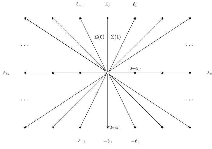
with Σ(n) lying between ℓn and ℓn+1 as before. The result is illustrated in Figure 3. With these
conventions the above involution identifies the ray diagrams for the BPS structures at (v, w) and (−v, w), so we obtain relations
Bn(−v, w, t) = Bn(v, w, t)−1, Dn(−v, w, t) = Dn(v, w, t).
· · · · · ·
· · · · · ·
ℓ0
ℓ−1 ℓ1
−ℓ∞ ℓ∞
−ℓ0
−ℓ−1 −ℓ1
Σ(0) Σ(1)
2πiw
[image:17.612.130.480.57.304.2]2πiv
Figure 2. The ray diagram associated to a point (v, w)∈M−.
We also consider the degenerate case when (v, w)∈M0. By applying theZ-action we can reduce
to the case when v/w∈ (0,1). We set ℓ =R>0·2πiw and define H =h·ℓ. The only active rays
are ±ℓ, and the wall-crossing formula implies that the (partially-defined) BPS automorphism S(ℓ) coincides with the map S(Σ) considered above. The Riemann-Hilbert problem is
Problem 3.6. Fix (v, w)∈ M0 with v/w ∈(0,1). Find holomorphic functions B(t) and D(t) on
the region
V=C∗\(R>0·w)
satisfying the following properties:
(i) As t→0 in any closed subsector of V one has
B(t)→1, D(t)→1.
(ii) There exists k >0 such that for any closed subsector of V
|t|−k <|B(t)|,|D(t)|<|t|k, |t| ≫0.
(iii) Note that V∩ −V=H⊔ −H. In the region H there are relations
B(t)·B(−t) =Y
n≥0
1−xqn
·Y n≥1
1−x−1qn)−1,
D(t)·D(−t) =Y
n≥0
1−xqnn
·Y n≥1
1−x−1qnn
·Y k≥1
1−qk−2k
,
4. Double and triple sine functions
In this section we introduce some special functions which will be used in the next section to solve the conifold Riemann-Hilbert problem introduced in the last section. The relevant special functions are, up to some exponential factors, the double sine function, and the triple sign function with two equal parameters.
Multiple sine functions are usually defined using the multiple gamma functions of Barnes [3]. Both are functions of a variable z ∈C and r parameters ω1,· · · , ωr∈C∗. One has
sinr(z|ω1,· · · , ωr) = Γr(z|ω1,· · · , ωr)·Γr
Xr
i=1
ωi−z|ω1,· · · , ωr
(−1)r
.
For definitions and results on multiple gamma and sine functions we recommend [15, 21, 25,29].
4.1. Double sine function. We begin by considering a function of z ∈ C and two parameters
ω1, ω2 ∈C∗. We shall use the notation
x1 = exp(2πiz/ω1), x2 = exp(2πiz/ω2), q1 = exp(2πiω2/ω1), q2 = exp(2πiω1/ω2). (20)
Our function is obtained by multiplying the double sine function by an exponential prefactor. The definition is
F(z|ω1, ω2) =e−
πi
2·B2,2(z|ω1,ω2)·sin
2(z|ω1, ω2), (21)
where B2,2(z|ω1, ω2) is the multiple Bernoulli polynomial
B2,2(z|ω1, ω2) =
z2
ω1ω2
− 1 ω1
+ 1
ω2
z+1 6
ω
2
ω1
+ω1
ω2
+1 2.
Up to trivial changes of variables the function F(z|ω1, ω2) coincides with the Fadeev dilogarithm
appearing in the work of Fock and Goncharov on cluster theory [11].
Although F(z|ω1, ω2) is a single-valued function of z ∈ C for fixed values of ω1, ω2 ∈ C∗, to
make it a single-valued function of all three parameters we must introduce a cut-line. We will therefore only consider the function under the additional assumption thatω2/ω1 ∈/ R<0.
Proposition 4.1. The functionF(z|ω1, ω2) is a single-valued meromorphic function of variables
z ∈C and ω1, ω2 ∈C∗ under the assumption ω2/ω1 ∈/ R<0. It has the following properties:
(i) The function is regular and non-vanishing except at the points
z =aω1+bω2, a, b∈Z,
which are zeroes if a, b≤0, poles if a, b >0, and otherwise neither.
(ii) It is symmetric in the arguments ω1, ω2:
F(z|ω1, ω2) =F(z|ω2, ω1),
(iii) It satisfies the two difference relations:
F(z+ω1|ω1, ω2)
F(z|ω1, ω2)
= 1
1−x2
, F(z+ω2|ω1, ω2) F(z|ω1, ω2)
= 1
1−x1
. (22)
(iv) There is a product expansion
F(z|ω1, ω2) =
Y
k≥0
(1−x1q1−k)−1·
Y
k≥1
(1−x2q2k),
valid when Im(ω1/ω2)>0.
(v) When Re(ωi)>0 and 0<Re(z)<Re(ω1+ω2) there is an integral representation
F(z|ω1, ω2) = exp
Z
C
ezs
(eω1s−1)(eω2s−1) ds
s
!
, (23)
where the contour C follows the real axis from −∞ to +∞ avoiding the origin by a small
detour in the upper half-plane.
Proof. Note that up to a trivial change of variables the double sine function coincides with the
hyperbolic gamma function of Ruijsenaars [28, 30] (see particularly equation (3.52) of [28]). The global properties of this function are covered by [30, Prop. III.5], and since the exponential prefactor in (21) does not affect these, this implies part (i).
The integral formula, part (v), is proved in [25, Prop. 2]. Property (ii) is then obvious by analytic continuation, but in any case this is a standard property of the double sine function: see [15, Appendix A].
For part (iii) we only have to check one relation, by symmetry. The double sine function satisfies the difference relation
sin2(z+ω1|ω1, ω2)
sin2(z|ω1, ω2)
= 1
2 sin(πz/ω2)
.
This can be found in [28, Prop. III.1] or [15, Equation (A.8)]. Combining this with the identity
B2,2(z+ω1|ω1, ω2)−B2,2(z|ω1, ω2) = 2B1,1(z|ω2) =
2z ω2
−1
gives (iii). Alternatively one can give a direct proof using the integral identity (v).
The product expansion, part (iv), is due to Shintani. It can be found in [25, Corollary 6] or [28,
Equation (3.58)].
4.2. Triple sine with repeated argument. We now consider another function of z ∈ C and
ω1, ω2 ∈C∗ related to the triple sine function. We define
G(z|ω1, ω2) =e
πi
6·B3,3(z+ω1|ω1,ω1,ω2)·sin
3 z+ω1|ω1, ω1, ω2
, (24)
where B3,3(z|ω1, ω2, ω3) is the multiple Bernoulli polynomial
B3,3(z|ω1, ω2, ω3) =
z3
ω1ω2ω3
− 3(ω1+ω2+ω3)
2ω1ω2ω3
+ω
2
1+ω22+ω32+ 3ω1ω2+ 3ω2ω3+ 3ω3ω1
2ω1ω2ω3
z− (ω1+ω2+ω3)(ω1ω2+ω2ω3+ω3ω1)
4ω1ω2ω3
.
Note that the function G(z|ω1, ω2) is not symmetric in ω1, ω2: we will use both the functions
G(z|ω1, ω2) andG(z|ω2, ω1) in what follows.
Proposition 4.2. The function G(z|ω1, ω2) is a single-valued meromorphic function of variables
z ∈C and ω1, ω2 ∈C∗ under the assumption ω2/ω1 ∈/ R<0. It has the following properties:
(i) The function is everywhere regular and vanishes only at the points
z =aω1+bω2, a, b∈Z,
with a <0 and b≤0, or a >0 and b ≥0.
(ii) It satisfies the symmetry relation
∂ ∂ω2
logG(z|ω1, ω2) =
∂ ∂ω1
logG(z|ω2, ω1), (25)
and is invariant under simultaneous rescaling of all three arguments.
(iii) It satisfies the difference relation
G(z+ω1|ω1, ω2)
G(z|ω1, ω2)
=F(z+ω1|ω1, ω2)−1. (26)
(iv) There is a relation
∂ ∂ω2
logF(z|ω1, ω2) =
∂
∂z logG(z|ω2, ω1). (27)
(v) When Re(ωi)>0 and −Re(ω1)<Re(z)<Re(ω1+ω2) there is an integral representation
G(z|ω1, ω2) = exp
Z
C
−e(z+ω1)s
(eω1s−1)2(eω2s−1) ds
s
!
, (28)
where as before, the contour C follows the real axis from −∞ to +∞ avoiding the origin
by a small detour in the upper half-plane.
Proof. The global properties follow from standard properties of mutiple sine functions [15], or can
be deduced from the corresponding properties of the function F(z|ω1, ω2) using the relations (27).
The integral representation, part (v), is proved in [25, Prop. 2], and the relations (ii) and (iv) are then immediate by differentiating under the integral sign and comparing with Prop. 4.1(v). Part
C+
C−
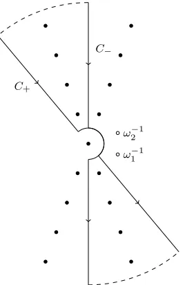
[image:21.612.242.376.55.261.2]ω−1 2 ω−11
Figure 3. The contours for the proof of Proposition 4.3.
4.3. Reflection relations. The following reflection properties will be needed later.
Proposition 4.3. When Im(ω1/ω2)>0 and z ∈C the following relations hold
F(z+ω2|ω1, ω2)·F(z|ω1,−ω2) =
Y
k≥0
1−x2q2k
·Y k≥1
1−x−21q2k−1
, (29)
G(z+ω2|ω1, ω2)·G(z|ω1,−ω2) =
Y
k≥1
1−x2q2k
k
·Y k≥1
1−x−21q2kk
, (30)
where x2 and q2 are defined in (20).
Proof. We start with (29). For definiteness, we can assume that z and the ω1, ω2 lie close to the
positive real axis: since the right-hand side of our relation clearly defines an analytic function for Im(ω1/ω2)>0, the result follows in general by analytic continuation. The contour C defining the
integral representation (23) can be rotated to point along a different ray ℓ = R>0·r, providing
that it does not hit the rays spanned by 2πi/ωi where the poles of the integrand lie, and providing
that
Re(ωis)>0, 0<Re(zs)<Re((ω1+ω2)s), (31)
for s ∈ ℓ, which ensures that the integrand decays exponentially as |s| → ∞ with s ∈ ±ℓ. Note that for small enough |z| the conditions (31) are equivalent to the assumption that the half-plane centered on ℓ contains the points ωi−1 and z−1.
Consulting Figure 3 it is easy to see that
F(z+ω2|ω1, ω2)·F(z|ω1,−ω2) = exp
Z
C+
e(z+ω2)s
(eω1s−1)(eω2s−1) ds
s +
Z
C−
ezs
(eω1s−1)(e−ω2s−1) ds
s
where C− and C+ are rotations of our standard contour C whose positive directions lie along
differ only by a sign, the expression in the exponential is just the sum of residues at the points
s= 2πim/ω2 for m∈Z\ {0}, taken with a positive or negative sign depending on the sign of m.
This residue is
2πi·Ress=2πim ω2
e(z+ω2)sds
(eω1s−1)(eω2s−1)s
= e
2πimz/ω2
m(e2πimω1/ω2 −1) =
xm
2
m(qm
2 −1)
.
Thus we obtain an expression
F(z+ω2|ω1, ω2)·F(z|ω1,−ω2) = exp
X
m≥1
−xm
2
m(1−qm
2 )
+X
m≥1
x−2mq2m
m(1−qm
2 )
= exp
− X m≥1,k≥0
1
mx m
2 qkm2 +
X
m≥1,k≥1
1
mx
−m
2 qkm2 )
=Y
k≥0
(1−x2q2k)·
Y
k≥1
(1−x−21qk2)−1,
which completes the proof of (29).
To prove (30) we follow the same strategy. Under the same conditions as before we get
G(z+ω2|ω1, ω2)·G(z|ω1,−ω2) = exp
Z
C+
−e(z+ω1+ω2)s
(eω1s−1)2(eω2s−1) ds
s +
Z
C−
−e(z+ω1)s
(eω1s−1)2(e−ω2s−1) ds
s
.
Once again the integrands differ only by a sign, so the expression in the exponential is just the sum of the residues at the points s= 2πim/ω2 for m ∈Z\ {0}, taken with a positive or negative
sign depending on the sign ofm. This time the residue is
2πi·Ress=2πim ω2
−e(z+ω1+ω2)sds
(eω1s−1)2(eω2s−1)s
= −e
2πim(z+ω1)/ω2
m(e2πimω1/ω2 −1)2 =
−xm2 q2m
m(1−qm
2 )2
.
Thus we obtain an expression
G(z+ω2|ω1, ω2)·G(z|ω1,−ω2) = exp
X
m≥1
−xm
2 qm2
m(1−qm
2 )2
+X
m≥1
−x−2mqm
2
m(1−qm
2 )2
.
= exp
X
m≥1,k≥1
−k mx
m
2 qkm2 −
X
m≥1,k≥1
k mx
−m
2 q2km)
=Y
k≥1
(1−x2qk2)k·
Y
k≥1
(1−x−21q2k)k,
which completes the proof.
4.4. Polylogarithm and zeta identities. The asymptotic expansions of the functions F and
G which we derive in Sections 4.5 and 4.6 below involve the polylogarithm and Riemann zeta functions. In this section we collect some simple integral identities involving these functions.
The polylogarithm Lik(x) is defined by the power series
Lik(x) =
X
n≥1
xn
nk, (32)
which is absolutely convergent in the unit disc. For k ≤ 0 the function Lik(x) is rational, and
regular except for a pole at x = 1. For k ≥ 1 the function Lik(x) has a single logarithmic
singularity at x= 1. We list the special cases
Li−1(x) =
x
(1−x)2, Li0(x) =
x
In what follows we shall only use expressions of the form Lik(e2πia), and will always assume that
Im(a)>0, so the power series (32) will suffice to define the polylogarithm, and the multi-valuedness of the analytic continuation of Lik(x) fork ≥1 will play no role.
Proposition 4.4. Take complex numbersz and ω1 satisfying0<Re(z)<Re(ω1)andIm(z/ω1)>
0. Then for each integerd ∈Z there is an expression
Z
C
ezs·s−d eω1s−1ds =
ω1
2πi
d−1
·Lid(e2πiz/ω1), (33)
where as before the contour C follows the real axis from −∞ to +∞, with a small detour around
the origin in the upper half-plane.
Proof. The integrand has poles at the points 2πin/ω1 for n∈Z, with residues
(2πi)·Ress=2πin ω1
ezs eω1s−1·
ds sd
!
=ω1 2πi
d−1
· e
2πinz/ω1 nd .
Note that the assumption Im(z/ω1) > 0 ensures that the power series expansion (32) defining
Lid(e2πiz/ω1) is absolutely convergent, and coincides with the sum of the contributions from the
poles in the upper half-plane. To give a rigorous proof we note that since the integrand decays exponentially as |Re(s)| → ∞there is a relation
Z
C0
ezs·s−d eω1s−1ds−
Z
CN
ezs·s−d eω1s−1ds=
ω1
2πi
d−1
· N
X
n=1
e2πinz/ω1
nd , (34)
where for each N ≥0 we denote by CN the shifted contour C+ 2Nπi/ω1. But
Z
CN
ezs·s−d
eω1s−1ds =e
2πiN z/ω1 ·N−d·
Z
C0 ezs eω1s−1 ·
s N + 2πi ω1 −d ·ds.
The integral on the right can be bounded independently ofN, so using the hypothesis Im(z/ω1)>0
again, we conclude that the integral overCN in (34) tends to 0 asN → ∞.
Note that differentiating (33) gives the relation
−
Z
C
e(z+ω1)s·s1−d
(eω1s−1)2 ds=
d dω1
ω1
2πi
d−1
·Lid(e2πiz/ω1)
. (35)
The analogue of (35) when z = 0 involves the Riemann zeta function. Recall that ζ(x) is a meromorphic function of x ∈ C which is regular except for a simple pole at x = 1. For integers
n≤ 0 one has
ζ(−n) = (−1)
n·Bn
+1
n+ 1 , (36)
where Bn+1 denotes the (n+ 1)th Bernoulli number.
Proposition 4.5. Takeω1 ∈C∗ with Re(ω1)>0. Then for all d∈Z one has the relation
−
Z
C
eω1s·s1−d
(eω1s−1)2 ds=
(d−1)·ζ(d)
2πi ·
ω1
2πi
d−2
where the contour C is as in Propositon 4.4, and in the case d= 1 the right-hand side of (37) is
defined by setting (d−1)·ζ(d) = 1.
Proof. When d≥2 the argument of Proposition 4.4 also applies with Re(z) = 0 and hence yields
Z
C s−d
eω1s−1ds=
ω1
2πi
d−1
·ζ(d).
The result then follows by differentiating with respect to ω1.
When d < 0 the integrand is regular at s = 0 so we may replace the integral along C by one along R. The symmetry under s ↔ −s then forces the integral to be zero unless d is odd. In that case the standard integral representation of the zeta function together with the duplication formula shows that
2
Z ∞
0
s−d
eω1s−1ds =
ω
1
2πi
d−1
·ζ(d).
Differentiating with repsect to ω1 then gives
−
Z
C
eω1s·s1−d
(eω1s−1)2ds =−2
Z ∞
0
eω1s·s1−d
(eω1s−1)2ds =
(d−1) 2πi ·
ω
1
2πi
d−2
·ζ(d).
Whend= 0 the identity (37) can be checked by a simple residue calculation. Since the integrand is invariant under s↔ −s we can combine the integral over C and −C to obtain
−
Z
C
eω1s·s
(eω1s−1)2ds=
1
2·(2πi) Ress=0
eω1s·s
(eω1s−1)2ds
= 1 2 · 2πi ω2 1 .
Since ζ(0) = −1/2 this agrees with (37). Finally, when d = 1 the integrand has an obvious primitive and we obtain
−
Z
C
eω1s
(eω1s−1)2ds=
1
ω1
·
1
eω1s−1
∞
−∞
= 1
ω1
,
which matches with our definition of the right-hand side of (37) in this case.
4.5. Asymptotic expansions as ω2 →0. In this section we give asymptotic expansions for the
functions F and Gas the parameter ω2 →0.
Proposition 4.6. Fix z ∈ C and ω1 ∈ C∗ with 0 < Re(z) < Re(ω1) and Im(z/ω1) > 0. Then
there are asymptotic expansions
logF(z|ω1, ω2)∼
X
k≥0
Bk·ω2k−1
k! ·
2πi
ω1
k−1
·Li2−k(e2πiz/ω1), (38)
logG(z|ω1, ω2)∼
X
k≥0
Bk·ωk2−1 k! ·
d dω1
2πi
ω1
k−2
·Li3−k(e2πiz/ω1)
, (39)
logG(z|ω2, ω1)∼
X
k≥0
(k−1)·Bk·ωk2−2 k! ·
2πi
ω1
k−2
·Li3−k(e2πiz/ω1), (40)
Proof. We focus first on (38), the other parts will then follow by a similar argument. Using the
integral formula (23) and the Laurent expansion
1
eω2s−1 =
X
k≥0
Bk·(ω2s)k−1
k! = 1
ω2s
−1
2 +
ω2s
12 +· · · , (41)
gives an expression
logF(z|ω1, ω2) =
Z
C
ezs
(eω1s−1)(eω2s−1) ds
s =
Z
C
X
k≥0
Bk·ω2k−1·sk−1
k! ·
ezs eω1s−1
ds s .
The result then follows formally by exchanging the order of integration and summation and using the identity (33).
To justify this we must prove that for N >0
1
ω2N−1
Z
C
1
eω2s−1− N
X
k=0
Bk·(ω2s)k−1
k!
· e zs
eω1s−1 · ds
s →0 (42)
as ω2 → 0 in the closed subsector Σ. Since F is invariant under rescaling all variables we can
assume that |ω1|<1. Let us rewrite the left-hand side of (42) as
ω2·I(ω2) =ω2·
Z
C
RN(ω2s)·
sN ·ezs eω1s−1·
ds
s , (43)
where RN denotes the meromorphic function
RN(x) =
1
xN ·
1
ex−1− N
X
k=0
Bk·xk−1
k!
.
We are reduced to proving that the integral I(ω2) is bounded as ω2→ 0 in Σ.
The function RN(x) is regular on the unit disc and on Σ, and tends to 0 as |x| → ∞ with
±x∈Σ. Thus there is a constant K >0 such that
±x∈Σ or |x|<1 =⇒ |RN(x)|< K.
Since we assumed that |ω1| <1, we can take the contour C in (43) to consist of the union of the
segments (−∞,1) and (1,∞) of the real axis, together with the intersection of the unit circle with the upper half-plane. It follows that
s∈C and ω2 ∈Σ with|ω2|<1 =⇒ |RN(ω2s)|< K.
This then gives a bound
|I(ω2)|< K·
Z C
sN ·ezs eω1s−1·
ds s <∞,
independently of ω2. This completes the proof of (38).
The other two expansions can be derived in exactly the same way. For (39) we use the same Laurent expansion (41) and the identity (35), and for (40) we use the Laurent series
eω2s
(eω2s−1)2 =
X
k≥0
(1−k)·Bk·(ω2s)k−2
k! =
1 (ω2s)2
− 1
12 + 1 240(ω2s)
obtained by differentiating (41), together with the identity (33).
Note that the expansions of Proposition4.6 are related by the identities (25) and (27). We shall also need the following analogues of the expansions (39) and (40) whenz = 0.
Proposition 4.7. Fix ω1 ∈C∗ with Re(ω1)>0. Then there are asymptotic expansions
logG(0|ω1, ω2)∼
ζ(3)
πi · ω1
2πiω2
− πi
24+
X
k≥2
(−1)k−1·Bk·Bk
−2
(2πi)·k! ·
2πiω2
ω1
k−1
, (45)
logG(0|ω2, ω1)∼ −ζ(3)·
ω1
2πiω2
2 + 1 12log ω1 ω2 +X
k≥2
(−1)k−1·Bk·Bk
−2
k·(k−2)!·(k−2)·
2πiω2
ω1
k−2
, (46)
valid as ω2 →0 in any closed subsector of the half-plane Re(ω2)>0.
Proof. The expansion (45) is proved in exactly the same way as (40), replacing the identity (35)
with (37). To prove (46) we first apply the argument of Proposition 4.6 to the integral
∂ ∂ω1
logG(0|ω2, ω1) =
Z
C
e(ω1+ω2)sds
(eω1s−1)2(eω2s−1)2,
using the Laurent series (44) and the identity (37). This gives
ω2·
∂ ∂ω1
logG(0|ω2, ω1)∼ −
X
k≥0
Bk·(k−1)(k−2)·ζ(3−k) (2πi)·k! ·
2πiω2
ω1
k−1
. (47)
Integrating term-by-term and using the identity (36) then gives the result.
4.6. Asymptotic expansions as ω2 → ∞. We shall also need the asymptotic expansions of the
functions F and G as ω2 → ∞. These involve the Bernoulli polynomials Bn(x), which can be
defined by the Laurent expansion (51) below.
Proposition 4.8. Fix z ∈C andω1 ∈C∗ satisfying0<Re(z)<Re(ω1)and Im(z/ω1)>0. Then
there are asymptotic expansions
logF(z|ω1, ω2)∼ −
πi
12 ·
ω2
ω1
+B1(z/ω1)·log(ω2) +O(1) (48)
logG(z|ω1, ω2)∼
ζ(3) 4π2 ·
ω2 2 ω2 1 + πi 12· zω2 ω2 1 +1
2log(ω2)·
d dω1
(ω1·B2(z/ω1)) +O(1) (49)
logG(z|ω2, ω1)∼ −
ζ(3) 2π2 ·
ω2
ω1
− iπ
12·B1(z/ω1) +
X
k≥2
(−1)k·Bk(z/ω
1)·Bk−2
k!·(2πi) ·
2πiω1
ω2
k−1
(50)
valid as ω2 → ∞ in any closed subsector of the half-plane Re(ω2)>0.
Proof. Let us start with (50). Using the integral representation (28) we have
logG(z|ω2, ω1) =
Z
C
−e(z+ω2)s
(eω1s−1)(eω2s−1)2 ·
Applying the Laurent expansion
ezs eω1s−1 =
X
k≥0
Bk(z/ω1)·(ω1s)k−1
k! , (51)
gives an expression
logG(z|ω2, ω1) =
Z
C
X
k≥0
Bk(z/ω1)·(ω1s)k−1
k! ·
−eω2s
(eω2s−1)2 ·
ds s .
Exchanging the order of integration and summation, and using (37) gives
logG(z|ω2, ω1)∼
X
k≥0
Bk(z/ω1)
k! ·
2πiω
1
ω2
k−1
· (2−k)·ζ(3−k)
2πi ,
where as usual we set (2−k)·ζ(3−k) = 1 when k = 2. Using the identity (36) this expression reduces to (50).
To justify this we must show that for N ≫0
ωN2 −1·
Z
C
ezs eω1s−1−
N
X
k≥0
Bk(z/ω1)·(sω1)k
k!
!
· −e ω2s
(eω2s−1)2 ·
ds
s →0 (52)
as ω2 → ∞in a closed subsector Σ of the right-hand half-plane. We can rewrite this as
1
ω2
·I(ω2) =
1
ω2
·
Z
C
RN(s)
sN ·
−eω2s·(ω
2s)N
(eω2s−1)2 ·
ds s ,
where RN(s) denotes the expression in brackets in (52). Now we proceed as in the proof of Proposition 4.6. The function f(s) =RN(s)/sN is regular near s= 0 and is bounded on the real
axis as |s| → ∞. We can therefore find a bound |f(s/|ω2|)| < K for s ∈ C independently of ω2
satisfying |ω2|>1. Thus
|I(ω2)|< K·
Z C
eηs·(ηs)N
(eηs−1)2 ·
ds s ,
where η = ω2/|ω2| lies on the intersection of the unit circle with the sector Σ. Since this is a
compact subset of C we can find a uniform bound. For (48) we apply the same argument to the integral
∂ ∂ω2
logF(z|ω1, ω2) =
Z
C
−e(z+ω2)sds
(eω1s−1)(eω2s−1)2
to obtain an expansion
∂ ∂ω2
logF(z|ω1, ω2)∼ −
πi
12ω1
+ B1(z/ω1)
ω2
+X
k≥2
(−1)k−1·B
k(z/ω1)·Bk−1
k!·ω2
·
2πiω1
ω2
k−1
.
Integrating with respect to ω2 gives (48). Similarly, for (49) we use the integral
∂ ∂ω2
logG(z|ω1, ω2) =
Z
C
e(z+ω1+ω2)sds
together with (37) and the Laurent expansion
−e(z+ω1)s
(eω1s−1)2 =
X
k≥0
sk−2
k! ·
d dω1
Bk(z/ω1)ω1k−1
, (53)
obtained by differentiating (51), to get an expression
∂ ∂ω2
logG(z|ω1, ω2) =
ζ(3) 2π2 ·
ω2 ω2 1 + πi 12 · z ω2 1 +X
k≥2
(−1)k·Bk
−2·(2πi)k−2
k!·ω2k−1 · d dω1
Bk(z/ω1)·ω1k−1
.
Integrating with respect to ω2 then gives (49).
5. Solution to the Riemann-Hilbert problem
In this section we solve the conifold Riemann-Hilbert problems of Section 3 using the special functions F and Gintroduced in the last section.
5.1. Exponential pre-factors. Let us introduce the expression
H(z|ω1, ω2) =
G(z|ω1, ω2)
G(0|ω1, ω2)
. (54)
The functionsF and H will form the basis of the solution to the Riemann-Hilbert problem which we give in the next subsection. However, to give the correct limiting behavior as ω2 → 0 and
ω2 → ∞ we first need to modify them by some exponential prefactors. Let us define
F⋆(z|ω1, ω2) = F(z|ω1, ω2)·eQF(z|ω1,ω2), H⋆(z|ω1, ω2) =H(z|ω1, ω2)·eQH(z|ω1,ω2), (55)
where QF and QH are Laurent polynomials in ω2 given explicitly by
QF(z|ω1, ω2) =−
ω1
2πiω2
·Li2(e2πiz/ω1)−
1
2log(1−e
2πiz/ω1) + πi
12·
ω2
ω1
,
QH(z|ω1, ω2) =
d dω1 1 ω2 ω1 2πi 2
·(ζ(3)−Li3(e2πiz/ω1)) +
ω1
4πi(Li2(e
2πiz/ω1)−ζ(2))
− πi 12 · zω2 ω2 1 .
These expressions are uniquely determined by the asymptotic properties of the resulting functions
F∗ and H∗ (see the proof of Theorem 5.2 below).
Proposition 5.1. The functions F∗ and H∗ satisfy the difference relations
F∗(z+ω
1|ω1, ω2)
F∗(z|ω
1, ω2)
= 1
1−x2
, (56)
H∗(z+ω
1|ω1, ω2)
H∗(z|ω
1, ω2)
=F∗(z+ω
1|ω1, ω2)−1, (57)
and the reflection relations
F∗(z|ω1, ω2)·F∗(z|ω1,−ω2) =
Y
k≥0
1−x2q2k
·Y k≥1
1−x−21q2k−1
, (58)
H∗(z|ω1, ω2)·H∗(z|ω1,−ω2) =
Y
k≥1
1−x2qk2
k
·Y k≥1
1−x−21qk2
k
, (59)
Proof. Relations (56) and (57) follow directly from the corresponding relations (22) and (26) for
F and G. One just needs to check that
QF(z+ω1|ω1, ω2) =QF(z|ω1, ω2),
QH(z+ω1|ω1, ω2)−QH(z|ω1, ω2) =−QF(z|ω1, ω2),
but this is easily done. Note that the denominator in (54) has no effect because it is constant inz. Similarly, the relations (58) and (59) follow from the corresponding reflection properties in Proposition 4.3. Note that in (29) one has F(z+ω2|ω1, ω2) rather than simply F∗(z|ω1, ω2) as
in (58), and similarly forH. However this effect is precisely cancelled by the constant term of the Laurent polynomials QF and QH. In detail the relations are
logF(z+ω2|ω1, ω2)−logF(z|ω1, ω2) = log(1−e2πiz/w),
logG(z+ω2|ω1, ω2)−logG(z|ω1, ω2) =
d dω1
ω1
2πi·Li2(e
2πiz/ω1)
.
The first is immediate from the second relation of (22), whereas the second follows from the integral
representation (28) and the identity (35).
5.2. The solution. We can now give the solution to our Riemann-Hilbert problem.
Theorem 5.2. The unique solution to Problem 3.5 is
B(v, w, t) =F∗(v|w,−t), D(v, w, t) =H∗(v|w,−t), (60)
where the functions F∗ and H∗ are defined in the previous subsection.
Proof. We must first check that for a fixed (z, w) ∈ M+ these formulae do indeed define
non-vanishing holomorphic functions on the domain V(0) =H(−1)∪H(0). According to Proposition
4.1(i), the poles and zeroes of F(v|w,−t) occur when ±v = aw− bt with a, b ∈ Z≥0. Since
Im(v/w) 6= 0, such a relation implies that b > 0, and hence t lies on the ray ±v + aw for some a ≥ 0. This ray only lies in one of the half-planes H(−1) or H(0) (centered on the rays R>0·2πi(v−w) andR>0·2πivrespectively) if we take the negative sign anda = 0, but consulting
Proposition 4.1(i) more carefully, we see that this combination does not in fact correspond to a singularity of F. The same argument applies to G(v|w, t) using Proposition 4.2(i). Finally, note that the denominator in (54) causes no trouble, since by Proposition 4.2(i) again, G(0|w,−t) is regular and non-vanishing whenever t /∈R>0·w.
We now check the conditions of Problem 3.5 one by one. Parts (iii) and (iv) follow immediately from Proposition5.1, so it remains to prove the first two. Let Σ be a closed subsector of V(0). We
must show that for ω2 ∈Σ one has
(i) F⋆(z|ω
1, ω2) and G⋆(z|ω1, ω2)→1 as ω2 →0,
(ii) there exists k >0 such that for all |ω2| ≫0