Alfvén Waves in the Interplanetary Medium

Thesis by

John Winston Belcher

In Partial Fulfillrnent of the Requirements

For the Degree of

Doctor of Philosophy

California Institute of Technology Pasadena, California

1971

In Memory of my Father

JOHN COOK BELCHER

And to my Mother

ACKNOWLEDGMENTS

I wish to thank first and foremost my thesis adviser, Professor Leverett Davis, Jr., for his constant and unfailing guidance, advice, and encouragement during the course of this work.

I am deeply indebted to the Mariner V plasma experimenters, H. S. Bridge, A. J. Lazarus, and C. W. Snyder, for extensive use of their detailed plasma data. I am similarly indebted to the Mariner V magnetometer experimenters, P. J. Coleman, L. Davis, Jr., E. J. Smith, and D. E. Jones for access to and use of the magnetic field data. I am thankful to all of these experimenters for helpful and stimulating discussions.

-iv-ABSTRACT

A study of the wave properties of the microscale fluctuations (scale lengths of. 01 a. u. and less) in the interplanetary medium is presented using plasma and magnetic field data from Mariner V (Venus 196 7). The reduction procedure for the magnetic field data is summarized, and descriptions are given of the MIT plasma data and the merged plasma/field data tapes used in the analysis.

Observationally, it is found that large amplitude, non-sinusoidal Alfve'n waves propagating outward from the sun with a broad wavelength range from 103 to 5 x l06k.m dominate the micro-scale structure at least 50"'6 of the time. The waves frequently have an energy density comparable both to the unperturbed magnetic field energy density and to the thermal energy density. The pure st examples of the Alfve'n waves are found in high velocity solar wind streams and on their trailing edges. The largest cunplitude waves occur in the compression regions at the leading edges of high velo-city streams where the velovelo-city increases rapidly with time. In addition to being transverse to the average magnetic field direction, ~B' the Alfve'nic fluctuations generally exhibit a 10~ partial

polariza-tion in the ~Bx~ direction, where ~ is a unit vector radially away from the sun. Presumably magnetoacoustic wave modes occur, but they have not been identified, and, if pre s'ent, have a small average power of the order of 1096 or less of that in the Alfve'n mode.

interplanetary medium seem likely to be the undamped remnants of waves generated at or near the sun. The high level of wave activity

in high velocity, high temperature streams can be interpreted as evidence for the extensive heating of these streams by wave damping near the sun. The highest level of Alfve'nic wave activity in the com-pression regions at the leading edges of high velocity streams may be due either to the amplification of ambient Alfve'n waves in high velocity streams as they are swept into the compression regions or to the fresh generation of waves in these regions by the stream-stream collisions. The observed absence of the magnetoacoustic modes is evidence for their strong damping. The !:.BxeR anisotropy is viewed as due to the partial conversion of the Alfve'n waves to the damped magnetoacoustic modes as they are convected away from the sun; this process continually transfers energy from the micro-scale field fluctuations to the thermalized solar wind plasma.

-vi-TABLE OF CONTENTS

PART TITLE PAGE

I. INTRODUCTION ₁

1 3 3

6 7

II.

III • .

A. Large Scale Solar Wind Properties B.. MHD Fluctuations

1. Waves

z.

Discontinuities

c.

The Interpretation of Spacecraft Data

DATA REDUCTION

A

.

B.

c.

Recovery of Basic Magnetic Field Data 1. Master Data Library Tapes

2. Spacecraft Field Correction

3. R TN Coordinates and BAMF AT Tape Plasma Data and Magnetic Field Averages Plots of Magnetic Field and Plasma Data

OBSERVATIONS

A. Identification of the Alfvdn Wave Mode

9

9 9 10 12 12 13

21 21

1. Vector Correlations 21

2. Waves Versus Discontinuities 24

3. Frequency of Occurrence and Direction

B.

c.

Patterns of Wave Occurrence

1. Solar Wind Stream Structure

2. Correlations Between Three Hour

Averages of Plasma and Field Data

Statistical Properties of the Microscale

Field Fluctuations

I. Wave Spectra and Energy Densities

2. Microscale Anisotropies

33

33

52

57

57

62

IV. DISCUSSION OF OBSERVATIONS AND

QUALITA-v.

TIVE MODELS 80

A. Possible Origins of the Interplanetary Alfve'n

Waves 80

B.

Quasi-Stationary Stream Structure in the

Solar Wind

C. The Microscale Anisotropies and Wave

Damping

A WA VE DRIVEN SOLAR WIND MODEL

A. The WKB Wave Amplitudes

B. The Wave Modified Bernoulli Relation

C. Numerical Solutions and Discussion

95

101

101

107

113

I. Reference Level Parameters 113

-viii-3. Wave Modifications of the Static Solutions 130

4. Comparison with Observations 133

VI. SUMMARY 137

CHAPTER I

INTRODUCTION

A. Large Scale Properties of the Solar Wind

The interplanetary medium is a rarefied, essentially

collision-less plasma whose thermal and magnetic field energy densities are

usually of the same order of magnitude. A knowledge of the wave and

turbulence properties of this medium is essential for a reasonably

complete understanding of the solar wind, its energy sources, and its

interaction with cosmic rays, the planets, and the inter stellar region.

The wave properties of such plasmas are also of general astrophysi"".

cal interest, and spacecraft observations made in situ offer a unique

opportunity to study these properties directly. The present work is

primarily a phenomenological study of the small scale fluctuations

superimposed on the supersonic streaming motion of the solar wind,

using simultaneous plasma and magnetic field data from Mariner 5

(Venus 1967). We first review the large scale characteristics of the

solar wind, and consider briefly the types of waves and discontinuities

which might be expected to produce small scale fluctuations in the

in-terplanetary plasma. The Mariner 5 experiment and the data red

uc-tion process are then described. The identificauc-tion of Alfve'n waves on

the basis of both plasma and field data is demonstrated, and the

pro-perties of these waves, in particular their patterns of occurence with

respect to the large scale solar wind streams, are described.

Defi-ciencies in previous models of the small scale fluctuations are pointed

-2-sources of these fluctuations which explains many of their observed

properties. Finally, we discuss a quantitative mathematical model

for the interaction of the waves and the solar wind, and show that the

presence of the waves can be a significant factor in the dynamics of ·

the expanding solar corona.

The large scale properties of the solar wind are well known

(for a comprehensive review, see Hundhausen [ 1968 ]). The plasma

itself is a hot, ionized gas consisting primarily of electrons, protons,

and alpha particles (-4~ by number}; it is highly conducting and

es-sentially collisionless. The proton number density at la. u. is

typi-cally 8 particles/cm3, with an average field strength B of 8 y(l0-5

1

gauss}, giving an Alfve'n velocity (B/(4rrp)~) of around 50

km/

sec and

a proton cyclotron frequency (eB/m ) on the order of 1 cps. The solar

p

wind velocity at 1 a. u. averages 400

km/

sec, with only small (,.,..596)

deviations from purely radial flow. The magnetic field direction is on

the average along the classic spiral field direction [Parker, 1963

J,

with a hose angle of about 45

°

at the orbit of the earth.

The proton thermal speed averages around 40

km/

sec. Alpha

particles generally have the same thermal speed as the protons, and

are thus four times hotter. Electron temperatures are much more

difficult to measure, but they appear to be slightly higher than the

pro-ton temperatures, and show less variation. The adiabatic expansion

and cooling of the plasma as it flows outward results in a temperature

anisotropy aligned with the magnetic field> with the proton

tempera-ture parallel to the field direction typically a factor of 2. 0 higher

average only 1. 2 times higher than that perpendicular. The ratio of

proton thermal energy density to magnetic field energy density is

typically • 6 at 1 a. u.

There are large scale fluctuations about these average values

[Neugebauer and Snyder, 1966

J.

High velocity streams (""""600 km/sec)

with high proton thermal speeds ( ... 80 km/ sec) and low densities

(.-5/cm 3) are interspersed with low velocity streams (""300 km/ sec)

which are colder ( ... 30 km/sec) and more dense (""'25/cm3). The

us-ual duration of one of these streams is on the order of two days and

longer. The patterns of occurence of the smaller scale plasma waves

are closely related to these large scale streaming patterns. The

na-ture of this relationship is discussed in subsequent chapters.

B. MHD Fluctuations

Irregular smaH scale fluctuations in the magnetic field and

ve-locity are usually superimposed on the large scale spiral field and

stream structure. In order to understand the probable physical nature

of these fluctuations, we briefly review the properties of small

amp-litude waves and abrupt discontinuities in the magnetohydrodynamic

(MHD) a ppr oxim ation.

1. Waves

The theory of small amplitude waves in a collisionless plasma

with a static magnetic field is extensive. Approaches to the problem

include the cold plasma approximation [Stix, 1962; Montgomery and

Tidman, 1964], the two-fluid approximatioi;- [Stringer, 1963 ], and,

-4-compared to the ion cyclotron frequency and of wavelengths long corn-pared to the gyroradius), the double adiabatic approximation [Chew, Goldberger, and Low, 1956]. We limit ourselves here to a brief de-scription of the three wave modes in the classical collision dominated MHD plasma theory. This approach is adopted for four reasons: (1) plasma instabilities and the presence of the magnetic field effectively replace particle-particle collisions in giving the plasma the collective bulk properties of a fluid; {2) the experimental data to be considered

satisfy the hydromagnetic condition as defined above; {3) the MHD ap-proach has been used with reasonable success in the past in connec-tion with interplanetary shocks and the earth's bow shock; (4) MHD wave theory is relatively simple, and seems adequate to describe the

observed wave properties of the medium.

In the isotropic MHD approximation there are three distinct wave modes -- the Alfvdn, the fast, and the slow, with frequencies

WA, W+• and

w_.

respectively. If B is the static background field, k

-o

-the propagation vector of -the wave, and 9 -the angle between B and k, _{-o ,....,} then the d~spersion relations for these three modes are given

[Thompson, 1962

J

by

w'A2

=

(k _- • _-o B )2 /4'1Tp

0 ( 1)

(2)

1

where VA= B /(4'1Tp )a is the Alfvdn velOcity, p is the mass density,

0 0 0

typically of the order of 50 km/ sec. The Alfve'n mode is purely

trans-verse, and is characterized by constant density and field strength and

by velocity and magnetic ile1d perturbations 3l.. and £_, respectively,

that are perpendicular to the plane of B and k.

-o - Thus band v axe

-

-parallel (or anti--parallel), and are connected by

b

=

±D v

- A- (3)

where

and the sign in Equation (3) is the sign of -~ • ]2

0• Both the fast and

slow modes (with 9

f.

0) are associated with fluctuations in density

and field strength; variations in field strength are in phase with those

in density for the fast mode, and 180° out of phase for the slow mode.

The fluctuations b and v are in the plane of k and B , with b normal to

- - - -o

-~in this plane. The perturbation

Y.

is connected to£ by a linear

ten-sorial relationship~ in general is not parallel to£,. and the ratio of

the magnitude of

J2.

to that of

z.

is

where cp is the angle between

z.

and ]2

0, and,w± is given by (2). The

detailed equations may be found in Coleman [

1967].

For the

singu-lar case in which k is colinear with B , the three modes reduce to two

- -o

simple, orthogonal Alfvdn modes, each characterized by Equations

(3) and (4), and a pure acoustic mode in which there is no magnetic

perturbation.

Equations (1) through (5) above apply to isotropic plasmas.

aniso-

-6-tropic plasma such as the solar wind, Equation ( 4) becomes

1

where

DA = l8l A ( 4ir po) 3

G

4lr_( Pl\ ...,-P,__.L_) ] - -}

®A=

1-B 2

0

(6)

(7)

and pl!· and p .1.. are the pressures parallel and normal to

;§

0,

respec-tively [Parker, 1957

J

2. Discontinuities

Discontinuities in the isotropic MHD approximation are most

conveniently treated in a frame in which the plane of the discontinuity

is at rest. The Rankine-Hugoniot conservation equations must hold

aero ss the discontinuity, and solutions to these equations [Landau and

Lipshitz, 1962] are of two types:

(1) Non-propagating. This category includes the contact and

the tangential discontinuities. The contact discontinuity is simply the

boundary between two media at rest which have different densities and

temperatures; the magnetic field and the kinetic pressure are

contin-uous across the discontinuity. The tangential discontinuity is the

boundary between two streaming media. The velocity and magnetic

field are tangential on both sides of the discontinuity, and can have

any change in both magnitude and direction. The total pres sure

(kin-etic plus magn(kin-etic) is conserved across the discontinuity, and the

dis-continuity does not propagate with respect to either media.

(2) Propagating. This category includes the fast and slow

shocks, and the rotational discontinuity (sometimes called the Alfve'n

pro-pagate at the fast magnetoacoustic, slow magnetoacoustic, and Alfvdn

velocities, respectively. The rotational discontinuity may be thought

of as a sharply crested Alfvdn wave. Fast and slow shocks are rarely

observed in the solar wind, and we will not treat them further here.

The basic discontinuities with which we are concerned are thus the

contact, the tangential, and the rotational.

C. The Interpretation of Spacecraft Data

There are well-known difficulties in the interpretation of

spacecraft data. The plasma is convected past the spacecraft with a

velocity (~00 km/sec) that is high compared to the characteristic

MHD propagation speeds (,..,.50 km/ sec). Thus, all MHD disturbances

are convected outward whatever their true direction of propagation in

the rest frame of the plasma. Observed variations are primarily due

to the convection past the spacecraft of spatial structures which may

be either static and "frozen-in" or dynamic and slowly propagating.

In the frame of the wind, the two classes of structures have

substan-tially different properties, different origins, and different physical

natures; in the spacecraft frame, they may be quite difficult to

distin-guish on the basis of either magnetometer or plasma data alone. As

we shall see, an identification can usually be made on the basis of a

careful study of both magnetic field and plasma data. Throughout, we

use the term wave in a broad sense. In many instances the terms

Alfvdnic turbulence or rotational discontinuity might be more

appro-priate, although neither is fully descriptive of the phenomenon. In all

struc-

-8-tures, almost always non-sinusoidal and nonperiodic, which propa-gate in the rest frame of the solar wind.

Unless otherwise specified, time and frequencies given here-after refer to the spacecraft frame; these must be Doppler shifted to yield wavelengths and frequencies in the rest frame of the wind. For example, a wave structure propagating outward from the sun with the Alfvdn velocity VA superposed on the wind velocity VW and having an apparent period T in the spacecraft frame has a wavelength of

T(VW

+

VA) and period of T[(vw/V A)

+

1

J

in the rest frame of the wind. The fine scale structure we are concerned with has

character-istic scales of .01 a.u. and less; this corresponds to periods in the

CHAPTER II

DATA

REDUCTION

A. Recovery of the Basic Magnetic Field Data

1. Master Data Library Tapes

Mariner 5 (Venu.s 1967) was in operation from June 14, 1967,

to November 22, 1967 . . Magnetic field measurements were made by

a low-field, vector, helium magnetometer [Connor, 1968]. Three

triaxial field samples were obtained every 12, 6 seconds at the high

data rate, and every 50. 4 seconds at the low data rate. The high data

rate period extended from the beginning of the mission until July 24,

1967, after which time data were taken at the low rate; there are

ap-proximately 40 days of high rate data and 120 days of low rate data.

The fir st step in the analysis of the Mariner 5 data was the

reduction of the raw magnetometer data to a form which could be

used conveniently. The basic source of data for the Mariner 5

experi-ment is the Master Data Library (MDL) tapes. These tapes are

pro-vided by the Jet Propulsion Laboratory, and contain the entire tele

-metry stream from the spacecraft. The basic data sampling sequence

is called a frame, and consists of a number of individual measurements

for each experiment on board. The real time sampling length of the

frame is 12. 6 (50. 4) seconds at the high (low) rate, and each frame

has one time associated with it. Three vector readings of the mag

-netic field are returned per frame; they are spaced 1/7, 2/7, and 4/7

of the frame length after· the beginning of the frame . The three

-10-cartesian coordinate system. The attitude control jets in conjunction with sun and Canopus sensors keep the Z axis oriented along a radial line from the spacecraft to the sun, with the spacecraft/Canopus angle at -45° from the X-axis in the XY plane.

Measurements of the field components are returned in digital units (DN) in the range from +511 to -511. The conversion function from DN to gamma is very nearly linear with approximately . 4y per DN. Once every 2048 frames there is a 24 frame calibration sequence during which known fields of approximately ±40y and ±80y are produced at the position of the magnetometer; this calibration

in-sures the reliability of the DN to gamma conversion. Using a for-tran program XRPM provided by JPL, the magnetometer digital

readings in each frame, along with the frame time and various quality control words were read from the eleven MDL tapes comprising the Mariner 5 mission and written on two intermediate tapes, called

MARDI tapes. The MARDI tapes were then processed through various phases which successively: (1) converted DN measurements to gamma; (2) removed the calibration offsets so as to ,recover data during this sequence; (3) provided quality tags for each individual vector reading based on the number of bit errors in the telemetry stream for the frame and the consistency of that reading (within broad ranges) as compared to adjacent measurements.

2. Spacecraft Field Corrections

Smith, 1968]. Magnetometer readings~ are the sum of two vectors

M=

:§.+§.

where B is the true interplanetary magnetic field (often rapidly vary-ing) and £is the (unknown) spacecraft field (usually constant or only

slowly_ varying). Mathematically, £is chosen so as to minimize the high frequency variance in IM

I

during selected intervals. The method is based on the fact that previous experiments have shown the fine scale fluctuations in the interplanetary field to be primarily changes in direction, with relatively small changes in field strength. An appreciable error in the spacecraft field estimate for a given com-ponent wi 11 cause purely directional fluctuations to produce apparent field strength fluctuations. This fact, coupled with the above comment as to the nature of the variations, enables an inflight determination of the spacecraft field to be made. We subsequently show that this me-thod is quite reasonable in view of the predominant physical nature of the fine scale field fluctuations. The spacecraft field correction used for Mariner 5 is on the order of 10 y in magnitude and is considered

-12-3. RTN Coordinates and the BAMFAT Tape

Using trajectory and spacecraft orientation information

pro-vided by JPL, the field vectors :J2_ were rotated from the XYZ system

to orthogonal R TN solar polar coordinates, defined as follows: the

positive R direction is radially outward from the sun; the T direction

is parallel to the solar equatorial plane and positive in the direction

of planetary motion, and the N direction is northward along

E

X

I.

so

that R TN is right•handed. The R TN field components of the vectors,

with times and quality tags, were then written on the Basic Magnetic

Field Analysis Tape (BAMF AT). One tape contains the entire mission,

both high and low data rate. The basic unit is still one data frame,

packed into five 36 bit words, with 128 frames per BAMFAT record;

spacecraft trajectory information is written once per record. The

BAMF AT tape contains on the order of 300, 000 good quality

measure-ments of the interplanetary magnetic field.

B. Plasma Data and Magnetic Field Averages

The plasma probe on board Mariner 5 was flown by the MIT

plasma group, who have generously provided extensive and detailed

data from their experiment. The plasma detector, a modulated grid

Faraday cup [Lazarus, et al., 1967] points at the sun and measures

positive ion currents in 32 energy levels covering the range from

40 to 9400 ev, with a complete sampling cycle of about 5. 04 min at

the high data rate and 20. 16 min at the low. This includes a

direc-tional measurement from which the three components of the wind

collector cup. From the energy spectrum, Bridge and Lazarus

obtain estimates of N, the proton number density in cm -3, Y, the

vector bulk velocity of the solar wind protons, in

km/

sec, and VT'

1

the most probable proton thermal speed ( 2kT /m ) ~. in km/ sec.

p p

The plasma probe sampling sequence takes exactly 24 frames, and

thus spans 72 vector measurements of

12·

These magnetometer

measurements are averaged, and a merged plasma-field tape written

containing all of the above plasma parameters and averages of

mag-netic field components and magnitudes over the plasma probe sampling

period.

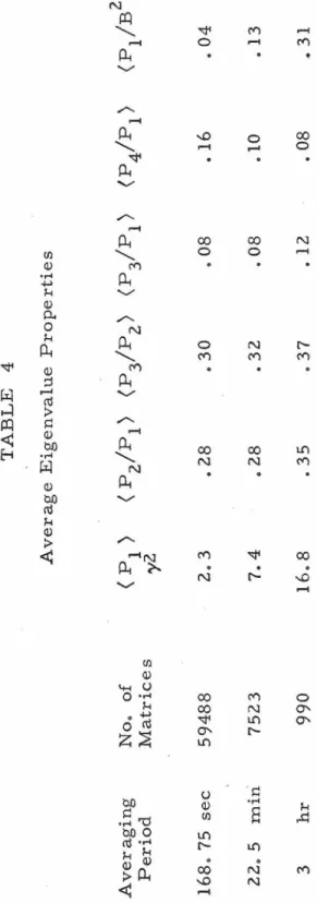
Using only good quality data from the BAMFAT tape, we also

compute averages and variances of the field data over intervals of

-9 -6 -3

168. 75 sec (2 day), 22. 5 min (2 day), 3 hr (2 day), and one day.

For each interval, (B), (

!

J?

I ),

and the matrix 2_ defined by

S ..

=

(B.B.) - (B.) (B.)

lJ l J l J

are calculated, where ( ) denotes averaging over the specified time

interval. This information is stored on magnetic tape.

C. Plots of Magnetic Field and Plasma Data

The Mariner 5 magnetic field data described above contain

fluctuations with characteristic times from 10 to 106 sec. One of

the most important steps in the data reduction is the choice of time

scales for data display, since vastly different physical processes

occur across the five orders of magnitude in time resolution. The

-14-three hours per plot, using the basic BAMFAT data; (2) one day per plot, using the 168. 75 sec. averages; (3) seven days per plot, using the 22. 5 min. averages; ( 4) twenty-seven days per plot, using the

three hour averages. The plasma parameters N, VT' and V are

plotted on scales of one day per plot, seven days per plot, and twenty-seven days per plot. Figures la through le show examples of these plots for each period. Note that the same data appear quite different on the various time scales. A wide range of time scales for data display is absolutely essential to the interpretation of interplanetary

5

·-:·.~

5

5

.

,,

,

·

.

.

.. ,::-= :~

):.-•• ., t; •

J

..

5

B

0

.

.

;··

•.

--

·

-

..

_..

--.

_·

_.

_.

_:·:: ... -

--

···

i i

l

~· I

.

""'~

: . ..i

.

.,.,..

,..!_.

.

-!

I

I

'A. •• -." ' ,..__ •• ·;,,-.,.,..r.,. ... ~_... .:.\ -~"' ... l·r"~...

.

; ""'

,

. ..--..:.,. • I • ' ~· , ,e::t. ·~ I

I .

..

I

I

i i

I

:~

-

.

·,-_-:

.·

..

...:

I

.,. 4.:f;~·.

··

.

...

.

..

..

\ -.·:~ ..

.

..

'

.

.

·

.

_.

..

_.

.

I

i

I

I

. ~::,-.~:,. l

Figure la. Three hours of basic magnetometer data from day 228 (9-12). This is during the low data rate part of the mission, so that readings are taken once in approximately 16 sec. BR' BN' and BT are solar polar

;

.

~

...

,,

,,

:\•;r. ~

·

..

.

;-...,:

..

<(

..

..

\

:\ ~

-16-.

..

'

1• ••

\•

.•

....

,.

_....

<( ...

::

·•.

...

.

.

'··

.

.:

:.~.

-r:::

:'.

"'

.:

·.:.

·.

> -: •

...

.

,

.

.~

...

\

~·.·"'":~:it..~ ·.

:

• • • -! .... ..

;v

,., ... v-... .

228

..

..

I

..r;: .

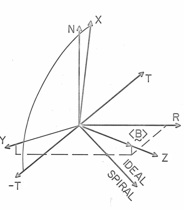
Figure le. Seven days of magnetic field data plotted using 22.5 minute

averages. BE and LA are magnetic field direction angles (in degrees).

0 0

BE is the angle out of the solar equatorial plane (-90 to 90 ) and LA

is the field angle in this plane measured from an idealized 45° spiral

field direction. A dark bar indicates this direction is outward along

the 45° spiral, and the absence of a bar indicates this direction is

inward along the spiral. BR, BT, BN are RTN solar polar field components

-18-~

~

..,

:~

!

0

a: w a: ~

...J en en CD

_)

I

z

en

ro N (\J

r--(\J

(\J

CD

(\J

(\J

()

lf) r-l

(\J

(\J Q)

(Y) (\J

(\J

(\J (\J (\J

a:

CD H ::l 00

•.-1

. I I

I

_ll _ _LI ___L_I -'---_l__J~_ l__j__I

~--' _Lf

i1

L1

~

I

ill

I I MAR l NER 5 I I ~ - L -1 I I 1 HM

GO~

I

J~ll

1

1111;, I :

~

J

J

-\~

l

~

40 1-n!INIJl l

20l--~~--·

-rov

hvt

l

500 VEL. 400

v~

r~~~~~~

'I

1~jtr/

3001---:---_J 20C

-20-900

SOLAR1 9 . 11 13 15 17 19 21 _{MARINER 5} 23 2'; 27

0

~,;---t-t-~--t~f~~~--+~~~~~

500

Vw

400

\vr""-

y

r/

\Jc\

;r

V'--1\

~!\,A

_,__,

Vz

~--""

~~~,A_/

..,,..,.

232 234 236 238. 240 242 244 246 248 200

100

0

Figure le. One solar rotation plotted using three hour averages. B is the magnetic field strength, N is the proton number density, VW is the solar wind velocity, and V is the proton thermal speed. ~ and A are

field direction angles.

~Tis

the field angle out of the solar equato- ·

rial plane, and A is a longitudinal angle in this plane measured from the R axis. P is the polarit6, and indicates whether the field has a

CHAPTER III OBSERVATIONS

A. Identification of the Alfve'n Wave Mode l. Vector Correlations

When interplanetary magnetic field data were first obtained more than eight years ago, the microscale structure was found to

be quite irregular, and it seemed plausible [Davis, 1966] that many of the features were propagating Alfve'n or magnetoacoustic waves. Coleman [ 196 7] carried out an extensive spectral and cross- spectral analysis of Mariner 2 (Venus, 1962) plasma and field data, and con-cluded that Alfve'n waves propagating away from the sun in the rest frame of the wind might account for a substantial fraction of the fluctuations with periods in the spacecraft frame from 10 to 1

o

4

seconds. This statistical analysis did not give patterns of occurence of the waves or explicit examples of the wave forms. The only ex-ample in which such waves were specifically identified was in a two hour segment of Mariner 2 data where Unti and Neugebauer [ 1968 J

demonstrated the existence of a quasi-sinusoidal Alfve'nic waveform with a period in the spacecraft frame of about 30 minutes. Belcher, Davis, and Smith [ 1969], in a preliminary analysis of Mariner 5

plasma and field data, identified outwardly propagating Alfve'nic wave trains as frequently occurring phenomena, although they are for the most part non-sinusoidal and aperiodic.

Ix 1— z

> > > Z

if) 010 100 1.0 10 0 0 co 0

N _Cii N

( -1 N Cii

L) Oct q• Oct ct- 0

..Ci _0 CO

cu a) •o Cu Cu s-1 e-' ICU >1 CJ)

(I)

• '0

• • ,--1 Cu

a) co

Cu

4-1 Cu co

O Cu 4J

0 0 nO 0

Cu •,-,1 cri N

a) -0

cl) 4,-, 0

a)

• C) .

Cr fa, a) _{u") ccs}

---.

• a u)

Cu Cu

tIO

to -0

Cu -r-1 Cu

▪ . r4 }.4

4J C1) a)

Cu 4-)

• 0 7:1 a

4-) 0 0 cn

0 0 0 O a) 0

o

a) 0 4_1

✓t) b,C) 0

Cu S-1

4-)

•

4-) Cu-4 0., -0

-0 0 Cu

(f) 0 ca cO

Cu 1-1 LL_

cn 4..)

Cu ,c) bo

— Lii c1,-1 a)

.-0 4..1

—Cu

t-U • a

Cu cn

.r.1

r--I 0.)

• PI+ "r-1

14-1 0 • 4 c.)

C) Lrl 4-)

4-)

- 4-1 (1)

CU 0

Cu cu bO

6.13 0 2

ct

a) a)

• 1113 O COCu

C.)

cn a) u)

• CO

• X

00 0C/) ca

4-) C)

• C) Cu

• CL, cl)

O Cu.. Cu a)

4-1 0

04 0

a) a

4-) .0 0 o

(I) (1)

• 4-1 E-1

• cO

0

0.) Cu 4.4

• a) a) cn

C)

b0

•

4-4 /:,0

co •,-,

field

.£?

and the plasma velocity

Y.

for a 24 hour period starting at 0400 on day 166 are shown. For each component, the average of that component over the 24 hour period has been subtracted; thus, the plots show the fluctuations about the average ((BR) = -1.

9y,

(BT)= l.4y, (BN) = 1.2y, (VR) = 427 km/sec; (VT) and (VN) have not yet been corrected for aberration due to the spacecraft motion). The two lower curves on the plot are proton number

den-sity N and magnetic field strength B (( B) = 5. 3y, (N) = 5. 4 cm-3). The Alfve'nic identification is based primarily on the fact that the vector relation between£ and

y_

given by Equation (3)

C!2.

= ±DA .:y:_) is satisfied. This period is one of the better examples of the waves and illustrates their most characteristic features -- close correla-tion between

J?.

and

y_,

variations in.£ comparable to the field strength, and relatively little variation in field strength or density, as is

ex-I

pected for the transverse Alfven mode. The fluctuations in Figure 2a must be predominantly Alfve'nic, since if there were a substantial

admixture of the fast or slow magnetoacoustic modes, there would be variations in field strength correlated with variations in the den-sity as well as with other quantities. In this case, the average mag-netic field is inward along the spiral and the correlation between£ and

y_

is positive; when the magnetic field is outward, the correlation in periods of good waves is negative. This indicates outward pro-pagation (see Equation (3)).

The scale ratio used for plotting the magnetic field and velo--1

-24--1;

Equation (3) of 6. 4 km sec gamma. This was determined by the condition that when this ratio is used for a fixed area plot of vR versus bR for all the data, the sum of the squares of the per-pendicular distances from the points to a line of unit slope is mini

-mized. (Mathematically this gives DA -l = avR/ 0bR, the ratio of the standard deviations.) The average values of N and Na (the alpha

-3

particle number density) during this period are 5. 4 cm and

- 3 . 6 . D -1

O. 4 cm , respectively; Equation ( ) with ®A= 1 gives A = 8.2

-1/

km sec gamma. We feel that the discrepancy between this pre-dieted value and the observed value of

6.

4 is significant and probably is due to the anisotropy in the pressure. This requires that

1 The average during this period of (ZkTP/mJ~, the most probable proton velocity, was observed to be 4 7 km/ sec, which corresponds to 4irp /B 2 = O. 5, where p is the mean proton

p 0 p

pressure. With reasonable values of the electron and alpha pressures and of the pressure anisotropy [ Hundhausen et al., 1967], the

required value of @A seems entirely reasonable. On other occasions when 13 = 8irp /B 2 is smaller, values of @A closer to unity would be

p 0

expected.

2. Waves Versus Discontinuities

R

T

N

.

-•.·

.

...

.:

...

... ----·. 1;. ~·

.

---·

-·

i-:··-·

.•

.T'"'9 . -.• ---,. -•1

.

.~ '•

...

·~.

.

..

:.r.1_

J_•-'-.... ~~ ·

.

.

.

~ -__ .; •. ··i ..

.·

~

. .

.

.

.

.

~-~

.

::-,,

..

,,.

.

.

.

.~"

....

~,...

:··

*.l" •• t ,... .. " ,,, •o• • I

..

~.

•,.._.

:~ ..

·.

,.

__

.

:·-;

· · ·~ -~··

....

:--.

...

....

• t ••. ,,,... •. ~~~·,r~~ .. ,_,.._~ .. "'"""'.'"'':~' I

166d

6h

52m23

5 i

I

5

g

~-..

.r

••

_

10/cc

l

.

.

..

~_

.

....1~ -·

'

·-•

-~'I.~-_

..

;,,,.~._4. ~ ~·--·.-:... . ..,.

..

··

..

-,

·~. .• 4. . . .( :-~--~., .. .,...,.;-...~ ... "··> .~ .,.,.. .. ·~"""'·

.

'

166

d

7h

32m43

5 ii

I

30km/s

.

.

..

•.•r.-:: :r.1...-. .m.-•-i.•! ... r:

r.

:rt-. ~. .. ,. t

-.

.

"'

·~~·

..

.

•..,,..:.,. ••

;o

.

1.1,.;.• , r--.\....,,..:. ... _· .-... i~:+:· ~~-~ ... ,... ... , ... "

I T

-26-gradual (Zb, ii) or discontinuous (Zb, i; Zb, iii); with abrupt changes within 4 seconds. As discussed below, we feel that all three examples are Alfve'nic, with continuous magnetic field lines, but with a discon-tinuity in direction in cases (Zb, i) and (Zb, iii). Such abrupt changes occur at a rate of about one per hour, and are enmeshed in more gradual changes.

The visual appearance of the field fluctuations is qualitatively different on the time scales of Figures Za and Zb. With the scale used in Figure Zb, the most prominent structures are the abrupt changes which tend to be preceded and followed by field values that appear nearly constant. For example, the structure in Figure (Zb, i) is more striking than that in (Zb, ii) even though both have about the same total change over the ten minute period, and both appear very

similar in Figure Za. On the time scale of Figure Za, the genuine high frequency abrupt changes do not stand out because they are in-distinguishable from large smooth changes when the data are aver-aged over 5. 04 minute intervals, and because the field no longer appears to remain steady before and after the jumps. Because the abrupt changes are the most visually striking features when field data are plotted at a high time resolution, even though they are relatively

fact, it has been suggested [Ness, 1969] that the fluctuations in Fig-ure Za are not dynamic structFig-ures propagating in the rest frame of the solar wind, but rather are an ensemble of spatially convected non-propagating MHD discontinuities in equilibrium. Since this point is of major importance in the interpretation of interplanetary magne-tic field fluctuations, we discuss it in some detail.

Consider the two non-propagating discontinuities in the iso-tropic MHD approximation, the contact and the tangential, as dis-cussed in I B above. The magnetic field is continuous aero ss the contact surface, which is of no interest to us, but both plasma and field parameters can change across the tangential discontinuity. Let n and t be subscripts denoting components normal and tangential, respectively, to the discontinuity surface and let [A] denote the change in A across the surface. A tangential discontinuity is char-acterized by Bn

=

0, Vn = 0, arbitrary and unrelated [Y.t] and [J?t], and any change in pressure and field strength subject to the condition

[p

+

B2 /8ir] = O. By constructing a series of special tangential dis-continuities, all having continuous density and field strength, with the plane of the discontinuity so chosen that B

=

0 on both sides, and

n

with [J?t

J

and[Yt

J

related by Equation (3) {where the sign is consis-tent from discontinuity to discontinuity and changes with the polarity), we can in fact make a structure such as in Figure Za which is static. None of these special conditions are required, but they are allowed by the tangential discontinuity equations. However, it is not clear

-28-place, and while it is possible to explain any one discontinuity in this

way, it is·hard to fit together a large number unless their shear

planes are all parallel. On the other hand, the Alfven I wave

hypothe-sis accounts for all of the observed properties in a straightforward

manner. When sufficiently sharp-crested, an Alfve'n wave can be

termed a rotational discontinuity. Such a discontinuity has continuous

density and field strength, Bn is non-zero and continuous, and [ f2.t J

and [Y.tJ are related by Equation (3). The only special conditions

needed to produce a data sequence as in Figure 2a is that all the

I

Alfven waves propagate outward.

The fluctuations in Figure 2a are thus viewed as purely

Alfve'nic, with occasional sharply crested Alfve'n waves enmeshed

in more gradual variations. This interpretation is in sharp contrast

to the non-propagating, filamentary model of the microscale structure

consisting of equilibrium regions of differing properties separated by

tangential discontinuities and convected outward from the sun by the

solar wind. Periods s.uch as in Figure 2a are usually found in high

velocity streams and on their trailing edges; they can last as long as

three days ( ... 7 a. u. of gas), and almost every discontinuity in that

time appears to be a sharply crested Alfve'n wave. We do not mean

to imply that all discontinuities in the solar wind are Alfve'nic, as

this is obviously not the case, but it appears that a high percentage

of them are, particular1y in certain regions (as discussed below).

Similarly, we feel that the filamentary or discontinuous model of the

must be applied with care. Even a tentative identification of struc-tures as dynamic or static must include a careful study of both mag-netic field and plasma data.

3. Frequency of Occurrence and Direction of Propagation It should be emphasized that the presence of the waves is very common, and tends to dominate the microstructur e of the inter-planetary medium. There are a total of about 25 days (a day being 24 consecutive hours} from the 160 day mission during which the Alfve'n waves are as 11_pure11 _{as those in Figure 2a; such periods tend} to occur in high velocity streams and on their trailing edges where typically the density is low and the temperature high. Other examples of the waves, in the presence of large scale velocity gradients,

static structures, shocks, polarity reversals, etc., are less clean, but they are still recognizably present. The identification of the waves during such periods is based on a visual inspection of plots of simultaneous plasma and field data at high time resolution. Alfven waves are adjudged to be pre sent if there is substantial high frequency fluctuation in the magnetic field, a good high frequency correlation

between BR and VR (low frequency correlations are influenced by slow linear trendsL and relatively little high frequenty fluctuation in density and field strength. In the following, we will state whether Alfve'n waves are present or not on the basis of such comparisons of plasma and field data, although such data will not always be repro-duced.

-30-waves, we have examined the distribution of p, the correlation

coefficient between BR and V R computed over six hour intervals

throughout the entire mission. Six hour intervals dominated by

outwardly propagating Alfve'n waves will have high values of Ip

I.

and

p will have the same sign as -P, where P is the polarity of the

aver-age field direction (+l for(_!?) outward along the spiral and -1 for

(_!?) inward along the spiral). For the 416 six-hour intervals in the

flight with more than 66 percent data return, 33 percent of the

intervals had J p J :::-: • 8 and 55 percent had Ip

I :::-: .

6. The sign of p

correlates extremely well with the polarity of the field. Table 1

lists the percentage of the six-hour intervals with

j

p

j

in the indicated

ranges for which pP is negative. Those six-hour intervals (112 out

of 416) for which (~) was not within 45

°

of a 45° spiral angle are

not included because of their poorly defined polarity. All but three

of the remaining six-hour intervals with

!Pl

:::-:.8 have pP <O,

indicat-ing outwardly propagatindicat-ing waves. Inspection of the three six-hour

intervals which are exceptions reveals that the high correlation and

positive pP are not caused by inwardly propagating waves, but by

slow linear trends during quiet times; such trends can cause a

spur-iously high value of l pl even when there are no wave-like or higher

frequency fluctuations present. Thus, Alfve'n waves in periods of

high

I

p I are essentially always outwardly propagating.

Periods for which

I

p

I

is not as high ( l pl

<

.

8) have pP

<

0

a large percentage of the time (see Table 1), but not as consistently

as do periods of higher correlation. The smaller values of J p J could

TABLE l

Range of

l pl

No. and percent Percent intervals

intervals in this with pP<O

range

.

o/.

2 44 ( 14) 66

• 2/. 4 41 ( 14) 68

• 4/. 6 47 (15) 83

. 6/. 8 76 (25) 83

• 8/1. 0 96 (32) 97

-32-trends, etc .• which can mask the effect of the correlation due to the waves. The intervals with pP

>

0 could be due to linear trends that cause a high value of J p J even when no waves are present. They could also be due to the presence of inwardly propagating Alfve'n waves. Suppose that we are studying microscale fluctuations which are exclusively due to an outwardly propagating Alfve'n wave of amplitude A+ and an inwardly propagating Alfve'n wave of amplitude A_, with no cross correlation between the two waveforms; then it is easily shown that pP

=

(A_ 2 - A+ 2)/(A _ 2 + A+ 2). For A_ 2 /A+ 2

=

I

2

1

2 2

1

2

l.

9,

pP

= -.

8, for A_ A+

=

1/3, pP

= -

.

5, and for A_ A+

=

l, pP = 0. Thus, the presence of inwardly propagating Alfve'n waves can significantly reduce

I

p

j

during periods of purely Alfve'nic fluctuations , and it is possible that six-hour intervals for which

Ip

j

~. 8 have inwardly propagating Alfve"nic components, perhaps

even with A_ 2 /A+ 2

> l in many of the cases with pP >

0. The impor-tant point is that although inwardly propagating Alfv~n waves may at times occur, they evidently never occur in an extremely pure form, since J p J ~ • 8 implies pP

<

O. Even though there may be periods in which there are both inward and outward Alfve'n waves, there are no periods with exclusively inward propagation, whereas periods with exclusively outward propagation evidently occur on the order of 30 percent of the time.

It is clear from Table 1 that Alfve'n waves propagating out-ward have a strong influence on the sign of p, even down to

l

p j = • 4.

together with the high percentage of times with

l

p j ~

•

6, strongly indicates that outwardly propagating Alfve'n waves dominate the microscale structure about 50 percent of the time. Coleman [1967] found precisely the same type of correlation shown in Table 1 in

a study of cross spectra between plasma and magnetic field data from Mariner II {Venus 1962), and also noted that this type of correspond-ence between p and P would be expected for outwardly propagating Alfve'n waves. The waves were thus also present in appreciable quantities in the interplanetary medium in 1962.

B. Patterns of Occurrence of the Waves 1. Solar Wind Stream Structure

I

As noted above, Alfven waves in the interplanetary medium have characteristic patterns of association with the large scale velocity structure of the solar wind. The macroscale properties of this stream structure were first discovered in the Mariner II data

[Neugebauer and Snyder, 1966; Snyder et al., 1963], and subsequent probes have confirmed these initial results [Wilcox and Ness, 1965]. Although the high velocity streams observed by Mariner V are not as long lived as those found previously, the streaming patterns in the Mariner V data are very similar to those observed by earlier

spacecraft, and exhibit the basic characteristics of fast and slow

•.

streams and their interactions. Figure 3 is a plot of three hour averages of various quantities over a 35 day period of the flight; V is the wind velocity, B is the magnetic field, N is the proton

w

VT

J~~v~~~~~AA~~

~-1Jl

,r-1

\rJ_JJL

j

I.

500.

(\

~Vf'"\r

ft/

\J-l..i\

~-Vw

~

\j

'\_~_)----Jl

l~n

·

·

~---.

A

·

,f

~

lr.l""-in...._

___

/

~"""--.11.-~~~---_,.,,.-~

-.j .,r ,_ J

-o.

~

12."

M\

___

~.JL~~~~~J~-,__,-\~

300. 20.

N

8

o.

225 230 235 240 245 250 255

I _{VJ ,.p.} I

velocity (2kT /m )~. High velocity regions in the solar wind tend p p

-36-non-Alfve'nic components. Regions with very large amplitude waves are indicated by the heavy bars in Figure 3.

Figure 4 is a detailed specific example of large scale stream-ing properties usstream-ing 40. 3 minute averages plotted over a seven day period from day 189 to 195.

crs

is the square root of the 40. 3 minute average of the total variance in the magnetic field components, in gamma, where the variances are computed over the plasma probe sampling period of 5. 04 minutes, and the total variance is the sum of the variances on the individual ax.es. Gaps in the curves occur during periods when data were not taken. The region of rapid velo-city increase at the leading edge of the high velovelo-city stream extends from appro.x.imate 1 y the beginning to the end of day 192. It is pre-ceded by relatively high densities, and is accoµipanied by enhanced temperatures and magnetic field fluctuations. The proton tern perature and the standard deviations in field components are low in the low velocity stream, are at a maximum in the region of rapid velocity increase, and decrease with velocity on the trailing edge of the stream. The proton number density falls to very low values inside the high

velocity stream proper {on day 193, for example) as compared to values in the low velocity stream {day i89). The density increase

o-s

VT Vw N

B

2.

J\r-!

o.

_{60. 20.}

~

500. 300.

,J

20.

l...>

o.

_10.

-38-of day 191 is accompanied by high field strengths, and thus is pro-bably associated with compression of the slow gas ahead of the fast stream. The relatively higher field strengths and densities in the latter half of day 192 (as compared with day 193) are similarly the probable result of the deceleration and compression of the fast gas as it runs into the more dense slow gas. (Day 192, hours 15 to 18, has an average density and field strength of 2. 6 cm -3 and 12. 9

-3 gamma, respectively, as opposed to average values of 1. 3 cm and 5.9 gamma on day 193, hours 0 to 3; although the field strength decrease in Figure 4 in the latter part of day 192 appears much larger than the density decrease, the relative change in the two quantities is the same.) In a later section we discuss further the dynamics of colliding stream structures.

Consider now the microscale fluctuations during this period. Their general level is indicated by the values of cr

5 in Figure 4; their character is indicated by comparisons of v and b similar to

-

-Figure 2a. These are shown for the most interesting part of the interval in Figure 5, in which lower frequency variations have been eliminated from all but the lower curve by subtracting from each point a smoothed low frequency mean obtained by averaging over two hours about the point. The upper curves are thus high frequency variations about running two hour means. We emphasize that the vector velocity data given here are preliminary, and we pre sent them only to demonstrate qualitative behavior. The variations in

1

velocity have been multiplied by (4'1T'(N) m ) ~ (See Equation (4)).

-40-where (N) is the smoothed proton number density for each point,

in order to normalize them to the magnetic field variations. B is

the magnitude of the average magnetic field before low frequency

averages are subtracted. Days 189 through 191 are very quiet

mag-netically, with little wave-like fluctuations at high frequencies;

how-ever, after the beginning of day 192 there is a high level of wave

activity that is seen in Figure 5 to become obviously Alfve'nic with

good correlations on all three axes after hour 15. The correlation

between 12. and

y_

is particularly impressive in view of the fact that

the plasma data are probably highly alai sed (changes in the

plasma properties during the measurement of the energy s pe ctr um)

as there is a large amount of variation in the magnetic field with

periods of less than five minutes, the plasma sampling period. For

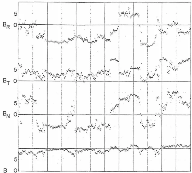
comparison Figure 6 is C:- point plot of 168. 75 sec. averages of the

·magnetic field during days 192 and 193, showing more clearly the

large amount of scatter in the field readings. The magnetic field

variations in the compression region (before hour 21 in Figure 6)

cannot be purely Alfve'nic, since there are comparatively large

fluctuations in B at higher frequencies. Even so, the power in the

field magnitude at higher frequencies is small compared to the power

in the field components, and the Alfve'n mode is obviously still

the dominant one. The polarity during this period is negative, and

thus the very large amplitude higher frequency fluctuations (periods

less than 2 hours) in the interaction region after hour 15 of day 192

are predominantly propagating outward. Before hour 15, in the mo st

14.--~~--,-~~-.-~~~~~---.-~~~~~~~~~~~~~~~~

,.,

'

.•

.•

.

j

I

. .

.

.·

-. .

.

·.

..:::

.. __ ::.:'

.l ·

> ...

. :::

:~

..

,/.:.v,:·:..'·/·.:~·:.\'.:.:

... \

.. .-.;

BR 0 , •· • --··.t.-•' · .. · " ·· ·

·..;:.:::.

.

.

:

.~,:

.

...

:.,::··

.. ?'\>

:';.";..:

..

, ..

--~

"

-:

.

l,

./

.:

~~:"'-.,,;..

·:,\

.. ·

·!";_:.:_

~

,:·: ·.. ., •• 0 / ~· ··-r....,.. • . ·14

+

-BT

oj

..

:'<',.

'·

..

' ..

;_.-,'...

••

,··.

•

-.

..

.

·'·'

.

f·: ···""''·'·' • • ' \ • 1.I ,,,_,. ·'··: •• • .,, •. . . •. ,

,,-~·· --~

••

··~

...

~.

;<-"." .. . . · 1

"'./<'':>-.;

i..

~-.

~

. ·);.,.. "':'"--··.-,; .. ' ... -.:,,' ' : • . 14-~.. -' ' :

.

::.

...

"

...

..

-..

.

.

:

..

'lo•

-42-not as good; this could be caused either by highly aliased plasma data, or by inwardly propagating Alfve'nic or magnetoacoustic wave modes. On days 193 and 194, the amplitude of the field fluctuations has decreased (this period is in the high velocity stream proper), and the correlation between b and v is extremely good {as in Figure 2a).

-The strength of the magnetic field fluctuations increases on all three axes as we move from the high velocity stream proper into the

compression region at its leading edge; note, however, that the normal component of the field has more power than the radial or the tangential in the compression region itself (see Figure 6). This be-havior appears to be a general property of field fluctuations in col-liding stream regions.

Other examples of stream structure in the solar wind have characteristics similar to the above. Figure 7 is a plot of days 233 through 239 in the same format as Figure 4, except that now cr

5

is the square root of the average total variance of the field components over 20. 16 minute intervals (the plasma sampling period at the low data rate used here). In this example, the leading edge of the high velocity stream beginning on day 236 is preceded by dense low velocity gas and the trailing edge of another high velocity stream. Again we point out that the density increase across days 234 and 235

~S

::t±:

~OU

UW\

~.HV

fn.~

4

Vr

:::~

~~JwlT~

v~

!1~

r

Vw

1100.1

.

r~~

A~I

·-

[..J-.

~M\r

.

•

~~

-I

300. 20.

-44-supply of the solar wind. The increase in density and field strength from the beginning to the middle of day 236 is probably the result of a dynamic compression of slow stream gas ahead of the fast stream, and the increase in field strength and density in going from day 237 to the last half of day 236 is probably due to the deceleration and compression of the fast gas as it runs into the slower, more dense gas ahead. Days 233. and 237 through 239 contain excellent examples of the pure outwardly propagating Alfve'n wave mode.

Days 234, 235, and the first half of 236 contain Alfve'n waves, but they are intermixed with more slowly varying structures which are associated with changes in density and field strength, and which may be static (note the large changes in field strength and density on these two and a half days in Figure 7 as compared to the four days men-tioned above). The last half of day 236 (the compressed fast gas) contains very large amplitude fluctuations which are primarily Alfve'nic . Figure 8 is a high time resolution plot of the field varia-tions in this period, showing in detail the enhanced field fluctuavaria-tions in the cam pression region. The normal component of the magnetic field has more power than the other components in the latter half of day 236.

Figure 9 is a third example of large scale stream structure although in this case the situation ahead of the fast stream is some-what chaotic. Day 285 after hour 6, and day 286 through the middle