Luminosity determination in pp collisions at root s=7 TeV using the ATLAS detector at the LHC

EUROPEAN ORGANISATION FOR NUCLEAR RESEARCH (CERN)

Eur. Phys. J. C (2016) 76: 653

DOI:10.1140/epjc/s10052-016-4466-1

CERN-PH-EP-2016-117 9th December 2016

Luminosity determination in

pp

collisions at

√

s

=

8 TeV using the ATLAS detector at the LHC

The ATLAS Collaboration

The luminosity determination for the ATLAS detector at the LHC during ppcollisions at √

s=8 TeV in 2012 is presented. The evaluation of the luminosity scale is performed using several luminometers, and comparisons between these luminosity detectors are made to as-sess the accuracy, consistency and long-term stability of the results. A luminosity uncertainty ofδL/L = ±1.9% is obtained for the 22.7 fb−1 ofppcollision data delivered to ATLAS at √

s=8 TeV in 2012.

c

2016 CERN for the benefit of the ATLAS Collaboration.

Reproduction of this article or parts of it is allowed as specified in the CC-BY-4.0 license.

1 Introduction

An accurate measurement of the delivered luminosity is a key component of the ATLAS [1] physics programme. For cross-section measurements, the uncertainty in the delivered luminosity is often one of the major systematic uncertainties. Searches for, and eventual discoveries of, physical phenomena beyond the Standard Model also rely on accurate information about the delivered luminosity to evaluate background levels and determine sensitivity to the signatures of new phenomena.

This paper describes the measurement of the luminosity delivered to the ATLAS detector at the LHC in ppcollisions at a centre-of-mass energy of √s = 8 TeV during 2012. It is structured as follows. The strategy for measuring and calibrating the luminosity is outlined in Sect.2, followed in Sect.3by a brief description of the detectors and algorithms used for luminosity determination. The absolute calibration of these algorithms by the van der Meer (vdM) method [2], which must be carried out under specially tailored beam conditions, is described in Sect.4; the associated systematic uncertainties are detailed in Sect. 5. The comparison of the relative response of several independent luminometers during physics running reveals that significant time- and rate-dependent effects impacted the performance of the ATLAS bunch-by-bunch luminometers during the 2012 run (Sect. 6). Therefore this absolute vdM calibration cannot be invoked as is. Instead, it must be transferred, at one point in time and using an independent relative-luminosity monitor, from the low-luminosity regime ofvdMscans to the high-luminosity condi-tions typical of routine physics running. Additional correccondi-tions must be applied over the course of the 2012 data-taking period to compensate for detector aging (Sect.7). The various contributions to the sys-tematic uncertainty affecting the integrated luminosity delivered to ATLAS in 2012 are recapitulated in Sect.8, and the final results are summarized in Sect.9.

2 Luminosity-determination methodology

The analysis presented in this paper closely parallels, and where necessary expands, the one used to determine the luminosity inppcollisions at √s=7 TeV [3].

The bunch luminosityL_bproduced by a single pair of colliding bunches can be expressed as

Lb= µfr σinel

, (1)

where the pile-up parameterµis the average number of inelastic interactions per bunch crossing, fris the

bunch revolution frequency, andσinelis theppinelastic cross-section. The total instantaneous luminosity

is given by

L=

nb

X

b=1

Lb=nbhLbi =nb

hµifr σinel .

Parameter 2010 2011 2012

Number of bunch pairs colliding (nb) 348 1331 1380

Bunch spacing [ns] 150 50 50

Typical bunch population [1011protons] 0.9 1.2 1.7

Peak luminosityL_peak[1033cm−2s−1] 0.2 3.6 7.7

Peak number of inelastic interactions per crossing ∼5 ∼20 ∼40 Average number of interactions per crossing (luminosity weighted) ∼2 ∼9 ∼21 Total integrated luminosity delivered 47 pb−1 5.5 fb−1 23 fb−1

Table 1: Selected LHC parameters forppcollisions at √s=7 TeV in 2010 and 2011, and at √s=8 TeV in 2012. Values shown are representative of the best accelerator performance during normal physics operation.

ATLAS monitors the delivered luminosity by measuringµvis, the visible interaction rate per bunch

cross-ing, with a variety of independent detectors and using several different algorithms (Sect. 3). The bunch luminosity can then be written as

Lb= µvis fr

σvis

, (2)

where µvis = ε µ, ε is the efficiency of the detector and algorithm under consideration, and the

vis-ible cross-section for that same detector and algorithm is defined byσvis ≡ ε σinel. Sinceµvis is a

dir-ectly measurable quantity, the calibration of the luminosity scale for a particular detector and algorithm amounts to determining the visible cross-sectionσvis. This calibration, described in detail in Sect.4, is

performed using dedicated beam-separation scans, where the absolute luminosity can be inferred from direct measurements of the beam parameters [2,4]. This known luminosity is then combined with the simultaneously measured interaction rateµvisto extractσvis.

A fundamental ingredient of the ATLAS strategy to assess and control the systematic uncertainties af-fecting the absolute luminosity determination is to compare the measurements of several luminometers, most of which use more than one algorithm to determine the luminosity. These multiple detectors and algorithms are characterized by significantly different acceptance, response to pile-up, and sensitivity to instrumental effects and to beam-induced backgrounds. Since the calibration of the absolute luminosity scale is carried out only two or three times per year, this calibration must either remain constant over ex-tended periods of time and under different machine conditions, or be corrected for long-term drifts. The level of consistency across the various methods, over the full range of luminosities and beam conditions, and across many months of LHC operation, provides a direct test of the accuracy and stability of the results. A full discussion of the systematic uncertainties is presented in Sects.5–8.

which are also recorded on a per-LB basis. Adding up the integrated luminosity delivered in a specific set of luminosity blocks provides the integrated luminosity of the entire data sample.

3 Luminosity detectors and algorithms

The ATLAS detector is discussed in detail in Ref. [1]. The two primary luminometers, the BCM (Beam Conditions Monitor) and LUCID (LUminosity measurement using a Cherenkov Integrating Detector), both make deadtime-free, bunch-by-bunch luminosity measurements (Sect. 3.1). These are compared with the results of the track-counting method (Sect.3.2), a new approach developed by ATLAS which monitors the multiplicity of charged particles produced in randomly selected colliding-bunch crossings, and is essential to assess the calibration-transfer correction from thevdMto the high-luminosity regime. Additional methods have been developed to disentangle the relative long-term drifts and run-to-run vari-ations between the BCM, LUCID and track-counting measurements during high-luminosity running, thereby reducing the associated systematic uncertainties to the sub-percent level. These techniques meas-ure the total instantaneous luminosity, summed over all bunches, by monitoring detector currents sensitive to average particle fluxes through the ATLAS calorimeters, or by reporting fluences observed in radiation-monitoring equipment; they are described in Sect.3.3.

3.1 Dedicated bunch-by-bunch luminometers

The BCM consists of four 8×8 mm2 diamond sensors arranged around the beampipe in a cross pattern atz = ±1.84 m on each side of the ATLAS IP.1 _{If one of the sensors produces a signal over a preset} threshold, ahitis recorded for that bunch crossing, thereby providing a low-acceptance bunch-by-bunch luminosity signal at |η| = 4.2 with sub-nanosecond time resolution. The horizontal and vertical pairs of BCM sensors are read out separately, leading to two luminosity measurements labelled BCMH and BCMV respectively. Because the thresholds, efficiencies and noise levels may exhibit small differences between BCMH and BCMV, these two measurements are treated for calibration and monitoring purposes as being produced by independent devices, although the overall response of the two devices is expected to be very similar.

LUCID is a Cherenkov detector specifically designed to measure the luminosity in ATLAS. Sixteen alu-minium tubes originally filled with C4F10gas surround the beampipe on each side of the IP at a distance of

17 m, covering the pseudorapidity range 5.6< |η|< 6.0. For most of 2012, the LUCID tubes were oper-ated under vacuum to reduce the sensitivity of the device, thereby mitigating pile-up effects and providing a wider operational dynamic range. In this configuration, Cherenkov photons are produced only in the quartz windows that separate the gas volumes from the photomultiplier tubes (PMTs) situated at the back of the detector. If one of the LUCID PMTs produces a signal over a preset threshold, that tube records a hit for that bunch crossing.

Each colliding-bunch pair is identified numerically by a bunch-crossing identifier (BCID) which labels each of the 3564 possible 25 ns slots in one full revolution of the nominal LHC fill pattern. Both BCM and

1_{ATLAS uses a right-handed coordinate system with its origin at the nominal interaction point in the centre of the detector,}

LUCID are fast detectors with electronics capable of reading out the diamond-sensor and PMT hit patterns separately for each bunch crossing, thereby making full use of the available statistics. These FPGA-based front-end electronics run autonomously from the main data acquisition system, and are not affected by any deadtime imposed by the CTP.2 They execute in real time several different online algorithms, characterized by diverse efficiencies, background sensitivities, and linearity characteristics [5].

The BCM and LUCID detectors consist of two symmetric arms placed in the forward (“A”) and backward (“C”) direction from the IP, which can also be treated as independent devices. The baseline luminosity algorithm is an inclusive hit requirement, known as the EventOR algorithm, which requires that at least one hit be recorded anywhere in the detector considered. Assuming that the number of interactions in a bunch crossing obeys a Poisson distribution, the probability of observing an event which satisfies the EventOR criteria can be computed as

PEventOR(µOR_vis)=NOR/NBC=1−e−µ OR

vis. (3)

Here the raw event countN_ORis the number of bunch crossings, during a given time interval, in which at least oneppinteraction satisfies the event-selection criteria of the OR algorithm under consideration, andNBCis the total number of bunch crossings during the same interval. Solving forµvisin terms of the

event-counting rate yields

µOR

vis =−ln

1− NOR

NBC

. (4)

Whenµvis1, event counting algorithms lose sensitivity as fewer and fewer bunch crossings in a given

time interval report zero observed interactions. In the limit where NOR/NBC = 1, event counting

al-gorithms can no longer be used to determine the interaction rateµvis: this is referred to assaturation. The

sensitivity of the LUCID detector is high enough (even without gas in the tubes) that the LUCID_EventOR algorithm saturates in a one-minute interval at around 20 interactions per crossing, while the single-arm inclusive LUCID_EventA and LUCID_EventC algorithms can be used up to around 30 interactions per crossing. The lower acceptance of the BCM detector allowed event counting to remain viable for all of 2012.

3.2 Tracker-based luminosity algorithms

The ATLAS inner detector (ID) measures the trajectories of charged particles over the pseudorapidity range|η|<2.5 and the full azimuth. It consists [1] of a silicon pixel detector (Pixel), a silicon micro-strip detector (SCT) and a straw-tube transition-radiation detector (TRT). Charged particles are reconstructed as tracks using an inside-out algorithm, which starts with three-point seeds from the silicon detectors and then adds hits using a combinatoric Kalman filter [6].

The luminosity is assumed to be proportional to the number of reconstructed charged-particle tracks, with the visible interaction rateµvis taken as the number of tracks per bunch crossing averaged over a

given time window (typically a luminosity block). In standard physics operation, silicon-detector data are recorded in a dedicated partial-event stream using a random trigger at a typical rate of 100 Hz, sampling each colliding-bunch pair with equal probability. Although a bunch-by-bunch luminosity measurement is possible in principle, over 1300 bunches were colliding in ATLAS for most of 2012, so that in practice only the bunch-integrated luminosity can be determined with percent-level statistical precision in a given

2_{The CTP inhibits triggers (causing deadtime) for a variety of reasons, but especially for several bunch crossings after a}

luminosity block. DuringvdMscans, Pixel and SCT data are similarly routed to a dedicated data stream for a subset of the colliding-bunch pairs at a typical rate of 5 kHz per BCID, thereby allowing the bunch-by-bunch determination ofσvis.

For the luminosity measurements presented in this paper, charged-particle track reconstruction uses hits from the silicon detectors only. Reconstructed tracks are required to have at least nine silicon hits, zero holes3 in the Pixel detector and transverse momentum in excess of 0.9 GeV. Furthermore, the absolute transverse impact parameter with respect to the luminous centroid [7] is required to be no larger than seven times its uncertainty, as determined from the covariance matrix of the fit.

This default track selection makes no attempt to distinguish tracks originating from primary vertices from those produced in secondary interactions, as the yields of both are expected to be proportional to the lu-minosity. Previous studies of track reconstruction in ATLAS show that in low pile-up conditions (µ≤1) and with a track selection looser than the above-described default, single-beam backgrounds remain well below the per-mille level [8]. However, for pile-up parameters typical of 2012 physics running, tracks formed from random hit combinations, known asfake tracks, can become significant [9]. The track selec-tion above is expected to be robust against such non-linearities, as demonstrated by analysing simulated events of overlaid inelasticppinteractions produced using the PYTHIA 8 Monte Carlo event generator [10]. In the simulation, the fraction of fake tracks per event can be parameterized as a function of the true pile-up parameter, yielding a fake-track fraction of less than 0.2% atµ = 20 for the default track selec-tion. In data, this fake-track contamination is subtracted from the measured track multiplicity using the simulation-based parameterization with, as input, thehµivalue reported by the BCMH_EventOR lumin-osity algorithm. An uncertainty equal to half the correction is assigned to the measured track multiplicity to account for possible systematic differences between data and simulation.

Biases in the track-counting luminosity measurement can arise from µ-dependent effects in the track reconstruction or selection requirements, which would change the reported track-counting yield per col-lision between the low pile-upvdM-calibration regime and the high-µ regime typical of physics data-taking. Short- and long-term variations in the track reconstruction and selection efficiency can also arise from changing ID conditions, for example because of temporarily disabled silicon readout modules. In general, looser track selections are less sensitive to such fluctuations in instrumental coverage; however, they typically suffer from larger fake-track contamination.

To assess the impact of such potential biases, several looser track selections, orworking points(WP), are investigated. Most are found to be consistent with the default working point once the uncertainty affecting the simulation-based fake-track subtraction is accounted for. In the case where the Pixel-hole requirement is relaxed from zero to no more than one, a moderate difference in excess of the fake-subtraction uncer-tainty is observed in the data. This working point, labelled “Pixel holes≤ 1”, is used as an alternative algorithm when evaluating the systematic uncertainties associated with track-counting luminosity meas-urements.

In order to all but eliminate fake-track backgrounds and minimize the associatedµ-dependence, another alternative is to remove the impact-parameter requirement and use the resulting superset of tracks as input to the primary-vertex reconstruction algorithm. Those tracks which, after the vertex-reconstruction fit, have a non-negligible probability of being associated to any primary vertex are counted to provide an alternative luminosity measurement. In the simulation, the performance of this “vertex-associated”

3_{In this context, a hole is counted when a hit is expected in an active sensor located on the track trajectory between the first}

working point is comparable, in terms of fake-track fraction and other residual non-linearities, to that of the default and “Pixel holes≤1” track selections discussed above.

3.3 Bunch-integrating detectors

Additional algorithms, sensitive to the instantaneous luminosity summed over all bunches, provide relative-luminosity monitoring on time scales of a few seconds rather than of a bunch crossing, allowing independ-ent checks of the linearity and long-term stability of the BCM, LUCID and track-counting algorithms. The first technique measures the particle flux from pp collisions as reflected in the current drawn by the PMTs of the hadronic calorimeter (TileCal). This flux, which is proportional to the instantaneous luminosity, is also monitored by the total ionization current flowing through a well-chosen set of liquid-argon (LAr) calorimeter cells. A third technique, using Medipix radiation monitors, measures the average particle flux observed in these devices.

3.3.1 Photomultiplier currents in the central hadronic calorimeter

The TileCal [11] is constructed from plastic-tile scintillators as the active medium and from steel absorber plates. It covers the pseudorapidity range |η| < 1.7 and consists of a long central cylindrical barrel and two smaller extended barrels, one on each side of the long barrel. Each of these three cylinders is divided azimuthally into 64 modules and segmented into three radial sampling layers. Cells are defined in each layer according to a projective geometry, and each cell is connected by optical fibres to two photomultiplier tubes. The current drawn by each PMT is proportional to the total number of particles interacting in a given TileCal cell, and provides a signal proportional to the luminosity summed over all the colliding bunches. This current is monitored by an integrator system with a time constant of 10 ms and is sensitive to currents from 0.1 nA to 1.2µA. The calibration and the monitoring of the linearity of the integrator electronics are ensured by a dedicated high-precision current-injection system.

The collision-induced PMT current depends on the pseudorapidity of the cell considered and on the radial sampling in which it is located. The cells most sensitive to luminosity variations are located near |η| ≈ 1.25; at a given pseudorapidity, the current is largest in the innermost sampling layer, because the hadronic showers are progressively absorbed as they expand in the middle and outer radial layers. Long-term variations of the TileCal response are monitored, and corrected if appropriate [3], by injecting a laser pulse directly into the PMT, as well as by integrating the counting rate from a137Cs radioactive source that circulates between the calorimeter cells during calibration runs.

The TileCal luminosity measurement is not directly calibrated by thevdMprocedure, both because its slow and asynchronous readout is not optimized to keep in step with the scan protocol, and because the luminosity is too low during the scan for many of its cells to provide accurate measurements. Instead, the TileCal luminosity calibration is performed in two steps. The PMT currents, corrected for electron-ics pedestals and for non-collision backgrounds4 and averaged over the most sensitive cells, are first cross-calibrated to the absolute luminosity reported by the BCM during the April 2012vdMscan ses-sion (Sect.4). Since these high-sensitivity cells would incur radiation damage at the highest luminosities encountered during 2012, thereby requiring large calibration corrections, their luminosity scale is trans-ferred, during an early intermediate-luminosity run and on a cell-by-cell basis, to the currents measured

4_{For each LHC fill, the currents are baseline-corrected using data recorded shortly before the LHC beams are brought into}

in the remaining cells (the sensitivities of which are insufficient under the low-luminosity conditions of vdMscans). The luminosity reported in any other physics run is then computed as the average, over the usable cells, of the individual cell luminosities, determined by multiplying the baseline-subtracted PMT current from that cell by the corresponding calibration constant.

3.3.2 LAr-gap currents

The electromagnetic endcap (EMEC) and forward (FCal) calorimeters are sampling devices that cover the pseudorapidity ranges of, respectively, 1.5<|η|<3.2 and 3.2<|η|<4.9. They are housed in the two endcap cryostats along with the hadronic endcap calorimeters.

The EMECs consist of accordion-shaped lead/stainless-steel absorbers interspersed with honeycomb-insulated electrodes that distribute the high voltage (HV) to the LAr-filled gaps where the ionization electrons drift, and that collect the associated electrical signal by capacitive coupling. In order to keep the electric field across each LAr gap constant over time, the HV supplies are regulated such that any voltage drop induced by the particle flux through a given HV sector is counterbalanced by a continuous injection of electrical current. The value of this current is proportional to the particle flux and thereby provides a relative-luminosity measurement using the EMEC HV line considered.

Both forward calorimeters are divided longitudinally into three modules. Each of these consists of a metallic absorber matrix (copper in the first module, tungsten elsewhere) containing cylindrical electrodes arranged parallel to the beam axis. The electrodes are formed by a copper (or tungsten) tube, into which a rod of slightly smaller diameter is inserted. This rod, in turn, is positioned concentrically using a helically wound radiation-hard plastic fibre, which also serves to electrically isolate the anode rod from the cathode tube. The remaining small annular gap is filled with LAr as the active medium. Only the first sampling is used for luminosity measurements. It is divided into 16 azimuthal sectors, each fed by 4 independent HV lines. As in the EMEC, the HV system provides a stable electric field across the LAr gaps and the current drawn from each line is directly proportional to the average particle flux through the corresponding FCal cells.

After correction for electronic pedestals and single-beam backgrounds, the observed currents are assumed to be proportional to the luminosity summed over all bunches; the validity of this assumption is assessed in Sect.6. The EMEC and FCal gap currents cannot be calibrated during avdMscan, because the instant-aneous luminosity during these scans remains below the sensitivity of the current-measurement circuitry. Instead, the calibration constant associated with an individual HV line is evaluated as the ratio of the absolute luminosity reported by the baseline bunch-by-bunch luminosity algorithm (BCMH_EventOR) and integrated over one high-luminosity reference physics run, to the HV current drawn through that line, pedestal-subtracted and integrated over exactly the same time interval. This is done for each usable HV line independently. The luminosity reported in any other physics run by either the EMEC or the FCal, separately for the A and C detector arms, is then computed as the average, over the usable cells, of the individual HV-line luminosities.

3.3.3 Hit counting in the Medipix system

readout chip. Each pixel in the matrix counts hits from individual particle interactions observed during a software-triggered “frame”, which integrates over 5 to 120 seconds, depending upon the typical particle flux at the location of the detector considered. In order to provide calibrated luminosity measurements, the total number of pixel clusters observed in each sensor is counted and scaled to the TileCal luminosity in the same reference run as the EMEC and FCal. The six MPX detectors with the highest counting rate are analysed in this fashion for the 2012 running period; their mutual consistency is discussed in Sect.6.

The hit-counting algorithm described above is primarily sensitive to charged particles. The MPX detectors offer the additional capability to detect thermal neutrons via6Li(n, α)3H reactions in a 6LiF converter layer. This neutron-counting rate provides a further measure of the luminosity, which is consistent with, but statistically inferior to, the MPX hit counting measurement [12] .

4 Absolute luminosity calibration by the van der Meer method

In order to use the measured interaction rateµvis as a luminosity monitor, each detector and algorithm

must be calibrated by determining its visible cross-sectionσvis. The primary calibration technique to

de-termine the absolute luminosity scale of each bunch-by-bunch luminosity detector and algorithm employs dedicatedvdMscans to infer the delivered luminosity at one point in time from the measurable parameters of the colliding bunches. By comparing the known luminosity delivered in thevdMscan to the visible interaction rateµvis, the visible cross-section can be determined from Eq. (2).

This section is organized as follows. The formalism of the van der Meer method is recalled in Sect.4.1, followed in Sect.4.2 by a description of thevdM-calibration datasets collected during the 2012 running period. The step-by-step determination of the visible cross-section is outlined in Sect.4.3, and each ingredient is discussed in detail in Sects.4.4 to4.10. The resulting absolute calibrations of the bunch-by-bunch luminometers, as applicable to the low-luminosity conditions ofvdMscans, are summarized in Sect.4.11.

4.1 Absolute luminosity from measured beam parameters

In terms of colliding-beam parameters, the bunch luminosityL_bis given by

L_b= f_rn₁n₂ Z

ˆ

ρ1(x, y) ˆρ2(x, y) dxdy , (5)

where the beams are assumed to collide with zero crossing angle,n1n2is the bunch-population product

and ˆρ1(2)(x, y) is the normalized particle density in the transverse (x–y) plane of beam 1 (2) at the IP.

With the standard assumption that the particle densities can be factorized into independent horizontal and vertical component distributions, ˆρ(x, y)=ρx(x)ρy(y), Eq. (5) can be rewritten as

Lb= frn1n2Ωx(ρx1, ρx2)Ωy(ρy1, ρy2), (6)

where

Ωx(ρx1, ρx2)=

Z

is the beam-overlap integral in the xdirection (with an analogous definition in the ydirection). In the method proposed by van der Meer [2], the overlap integral (for example in thexdirection) can be calcu-lated as

Ωx(ρx1, ρx2)=

Rx(0)

R

Rx(δ) dδ

, (7)

whereRx(δ) is the luminosity (at this stage in arbitrary units) measured during a horizontal scan at the

time the two beams are separated horizontally by the distanceδ, andδ = 0 represents the case of zero beam separation. Because the luminosityRx(δ) is normalized to that at zero separationRx(0), any quantity

proportional to the luminosity (such asµvis) can be substituted in Eq. (7) in place ofR.

Defining the horizontal convolved beam sizeΣx[7,13] as

Σx=

1 √

2π R

Rx(δ) dδ

Rx(0)

, (8)

and similarly forΣy, the bunch luminosity in Eq. (6) can be rewritten as

Lb=

frn1n2

2πΣxΣy

, (9)

which allows the absolute bunch luminosity to be determined from the revolution frequency f_r, the bunch-population productn1n2, and the productΣxΣywhich is measured directly during a pair of orthogonalvdM

(beam-separation) scans. In the case where the luminosity curveRx(δ) is Gaussian,Σxcoincides with the

standard deviation of that distribution. It is important to note that the vdM method does not rely on any particular functional form ofRx(δ): the quantities Σx andΣy can be determined for any observed

luminosity curve from Eq. (8) and used with Eq. (9) to determine the absolute luminosity atδ=0.

In the more general case where the factorization assumption breaks down, i.e. when the particle densities (or more precisely the dependence of the luminosity on the beam separation (δx, δy)) cannot be factorized

into a product of uncorrelatedxandycomponents, the formalism can be extended to yield [4]

ΣxΣy=

1 2π

R

Rx,y(δx, δy) dδxdδy

Rx,y(0,0)

, (10)

with Eq. (9) remaining formally unaffected. Luminosity calibration in the presence of non-factorizable bunch-density distributions is discussed extensively in Sect.4.8.

The measured product of the transverse convolved beam sizesΣxΣy is directly related to the reference

specific luminosity:5

Lspec≡

Lb

n₁n₂ = fr

2πΣxΣy

which, together with the bunch currents, determines the absolute luminosity scale. To calibrate a given luminosity algorithm, one can equate the absolute luminosity computed from beam parameters using Eq. (9) to that measured according to Eq. (2) to get

σvis=µMAX_vis

2πΣxΣy

n1n2

, (11)

whereµMAX

vis is the visible interaction rate per bunch crossing reported at the peak of the scan curve by that

particular algorithm. Equation (11) provides a direct calibration of the visible cross-sectionσvisfor each

algorithm in terms of the peak visible interaction rateµMAX_vis , the product of the convolved beam widths

ΣxΣy, and the bunch-population productn1n2.

In the presence of a significant crossing angle in one of the scan planes, the formalism becomes consider-ably more involved [14], but the conclusions remain unaltered and Eqs. (8)–(11) remain valid. The non-zero vertical crossing angle in some scan sessions widens the luminosity curve by a factor that depends on the bunch length, the transverse beam size and the crossing angle, but reduces the peak luminosity by the same factor. The corresponding increase in the measured value ofΣyis exactly compensated by the decrease inµMAX_vis , so that no correction for the crossing angle is needed in the determination ofσvis.

4.2 Luminosity-scan datasets

The beam conditions duringvdMscans are different from those in normal physics operation, with lower bunch intensities and only a few tens of widely spaced bunches circulating. These conditions are optim-ized to reduce various systematic uncertainties in the calibration procedure [7]. Three scan sessions were performed during 2012: in April, July, and November (Table2). The April scans were performed with nominal collision optics (β? =0.6 m), which minimizes the accelerator set-up time but yields conditions which are inadequate for achieving the best possible calibration accuracy.6 The July and November scans were performed using dedicatedvdM-scan optics with β? = 11 m, in order to increase the transverse beam sizes while retaining a sufficiently high collision rate even in the tails of the scans. This strategy limits the impact of the vertex-position resolution on the non-factorization analysis, which is detailed in Sect.4.8, and also reduces potentialµ-dependent calibration biases. In addition, the observation of large non-factorization effects in the April and July scan data motivated, for the November scan, a dedicated set-up of the LHC injector chain [16] to produce more Gaussian and less correlated transverse beam profiles.

Since the luminosity can be different for each colliding-bunch pair, both because the beam sizes differ from bunch to bunch and because the bunch populationsn1 andn2 can each vary by up to ±10%, the

determination ofΣxandΣyand the measurement ofµMAX_vis are performed independently for each

colliding-bunch pair. As a result, and taking the November session as an example, each scan set provides 29 independent measurements ofσvis, allowing detailed consistency checks.

To further test the reproducibility of the calibration procedure, multiple centred-scan7sets, each consisting of one horizontal scan and one vertical scan, are executed in the same scan session. In November for instance, two sets of centred scans (X and XI) were performed in quick succession, followed by two sets of off-axis scans (XII and XIII), where the beams were separated by 340µm and 200µm respectively in the non-scanning direction. A third set of centred scans (XIV) was then performed as a reproducibility check. A fourth centred scan set (XV) was carried out approximately one day later in a different LHC fill.

6_{Theβfunction describes the single-particle motion and determines the variation of the beam envelope along the beam}

traject-ory. It is calculated from the focusing properties of the magnetic lattice (see for example Ref. [15]). The symbolβ?denotes the value of theβfunction at the IP.

7_{Acentred(oron-axis) beam-separation scan is one where the beams are kept centred on each other in the transverse direction}

The variation of the calibration results between individual scan sets in a given scan session is used to quantify the reproducibility of the optimal relative beam position, the convolved beam sizes, and the visible cross-sections. The reproducibility and consistency of the visible cross-section results across the April, July and November scan sessions provide a measure of the long-term stability of the response of each detector, and are used to assess potential systematic biases in thevdM-calibration technique under different accelerator conditions.

4.3 vdM-scan analysis methodology

The 2012 vdM scans were used to derive calibrations for the LUCID_EventOR, BCM_EventOR and track-counting algorithms. Since there are two distinct BCM readouts, calibrations are determined sep-arately for the horizontal (BCMH) and vertical (BCMV) detector pairs. Similarly, the fully inclusive (EventOR) and single-arm inclusive (EventA, EventC) algorithms are calibrated independently. For the April scan session, the dedicated track-counting event stream (Sect.3.2) used the same random trigger as during physics operation. For the July and November sessions, where the typical event rate was lower by an order of magnitude, track counting was performed on events triggered by the ATLAS Minimum Bias Trigger Scintillator (MBTS) [1]. Corrections for MBTS trigger inefficiency and for CTP-induced deadtime are applied, at each scan step separately, when calculating the average number of tracks per event.

For each individual algorithm, thevdMdata are analysed in the same manner. The specific visible in-teraction rateµvis/(n1n2) is measured, for each colliding-bunch pair, as a function of the nominal beam

separation (i.e. the separation specified by the LHC control system) in two orthogonal scan directions (xandy). The value ofµvisis determined from the raw counting rate using the formalism described in

Sect.3.1or3.2. The specific interaction rate is used so that the calculation ofΣxandΣyproperly takes into

account the bunch-current variation during the scan; the measurement of the bunch-population product n1n2is detailed in Sect.4.10.

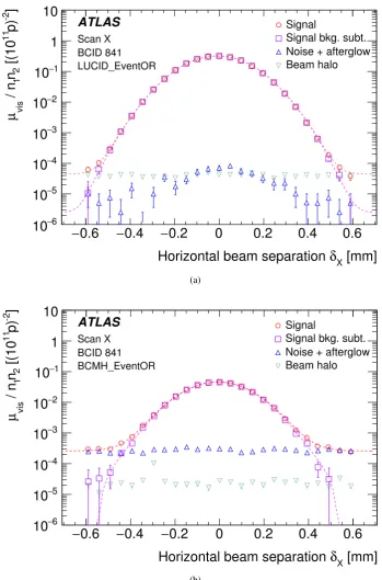
Figure1 shows examples of horizontal-scan curves measured for a single BCID using two different al-gorithms. At each scan step, the visible interaction rateµvisis first corrected for afterglow, instrumental

noise and beam-halo backgrounds as described in Sect.4.4, and the nominal beam separation is rescaled using the calibrated beam-separation scale (Sect.4.5). The impact of orbit drifts is addressed in Sect.4.6, and that of beam–beam deflections and of the dynamic-βeffect is discussed in Sect.4.7. For each BCID and each scan independently, a characteristic function is fitted to the corrected data; the peak of the fitted function provides a measurement ofµMAX_vis , while the convolved widthΣis computed from the integral of the function using Eq. (8). Depending on the beam conditions, this function can be a single-Gaussian function plus a constant term, a double-Gaussian function plus a constant term, a Gaussian function times a polynomial (plus a constant term), or other variations. As described in Sect.5, the differences between the results extracted using different characteristic functions are taken into account as a systematic uncer-tainty in the calibration result.

The combination of one horizontal (x) scan and one vertical (y) scan is the minimum needed to perform a measurement ofσvis. In principle, while theµMAX_vis parameter is detector- and algorithm-specific, the

convolved widths Σx and Σy, which together specify the head-on reference luminosity, do not need to

[mm]

X

δ

Horizontal beam separation

0.6

−

−

0.4

−

0.2

0

0.2

0.4

0.6

]

p)

[(10

n

/ n

µ

10

10

10

10

10

10

1

10

Signal bkg. subt. Noise + afterglow Beam halo

(a)

[mm]

δ

Horizontal beam separation

0.6

−

−

0.4

−

0.2

0

0.2

0.4

0.6

]

p)

[(10

n

/ n

µ

10

10

10

10

10

10

1

10

Signal bkg. subt. Noise + afterglow Beam halo

(b)

value ofµMAX

vis between the two scan planes is used. The correlations between the fitted values ofµMAXvis ,

ΣxandΣyare taken into account when evaluating the statistical uncertainty affectingσvis.

Each BCID should yield the same measured σvis value, and so the average over all BCIDs is taken

as the σvis measurement for the scan set under consideration. The bunch-to-bunch consistency of the

visible cross-section for a given luminosity algorithm, as well as the level of agreement betweenΣvalues measured by different detectors and algorithms in a given scan set, are discussed in Sect.5as part of the systematic uncertainty.

Once visible cross-sections have been determined from each scan set as described above, two beam-dynamical effects must be considered (and if appropriate corrected for), both associated with the shape of the colliding bunches in transverse phase space: non-factorization and emittance growth. These are discussed in Sects.4.8and4.9respectively.

4.4 Background subtraction

ThevdM calibration procedure is affected by three distinct background contributions to the luminosity signal: afterglow, instrumental noise, and single-beam backgrounds.

As detailed in Refs. [3,5], both the LUCID and BCM detectors observe some small activity in the BCIDs immediately following a collision, which in later BCIDs decays to a baseline value with several different time constants. This afterglow is most likely caused by photons from nuclear de-excitation, which in turn is induced by the hadronic cascades initiated by ppcollision products. For a given bunch pattern, the afterglow level is observed to be proportional to the luminosity in the colliding-bunch slots. DuringvdM scans, it lies three to four orders of magnitude below the luminosity signal, but reaches a few tenths of a percent during physics running because of the much denser bunch pattern.

Instrumental noise is, under normal circumstances, a few times smaller than the single-beam backgrounds, and remains negligible except at the largest beam separations. However, during a one-month period in late 2012 that includes the NovembervdMscans, the A arm of both BCM detectors was affected by high-rate electronic noise corresponding to about 0.5% (1%) of the visible interaction rate, at the peak of the scan, in the BCMH (BCMV) diamond sensors (Fig.1(b)). This temporary perturbation, the cause of which could not be identified, disappeared a few days after the scan session. Nonetheless, it was large enough that a careful subtraction procedure had to be implemented in order for this noise not to bias the fit of the BCM luminosity-scan curves.

Since afterglow and instrumental noise both induce random hits at a rate that varies slowly from one BCID to the next, they are subtracted together from the raw visible interaction rateµvis in each colliding-bunch

slot. Their combined magnitude is estimated using the rate measured in the immediately preceding bunch slot, assuming that the variation of the afterglow level from one bunch slot to the next can be neglected.

summing the contributions from the two beams. This background typically amounts to 2×10−4_(8×10−4₎

of the luminosity at the peak of the scan for the LUCID (BCM) EventOR algorithms. Because it depends neither on the luminosity nor on the beam separation, it can become comparable to the actual luminosity in the tails of the scans.

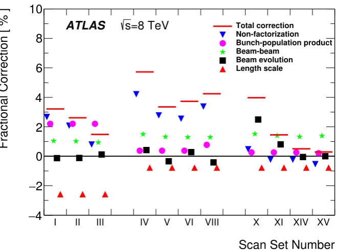
4.5 Determination of the absolute beam-separation scale

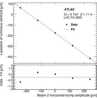
Another key input to thevdMscan technique is the knowledge of the beam separation at each scan step. The ability to measureΣdepends upon knowing the absolute distance by which the beams are separated during thevdMscan, which is controlled by a set of closed orbit bumps8applied locally near the ATLAS IP. To determine this beam-separation scale, dedicated calibration measurements were performed close in time to the April and July scan sessions using the same optical configuration at the interaction point. Such length-scale scans are performed by displacing both beams transversely by five steps over a range of up to ±3σnom_b , at each step keeping the beams well centred on each other in the scanning plane. The actual displacement of the luminous region can then be measured with high accuracy using the primary-vertex position reconstructed by the ATLAS tracking detectors. Since each of the four bump amplitudes (two beams in two transverse directions) depends on different magnet and lattice functions, the length-scale calibration scans are performed so that each of these four calibration constants can be extracted independently. The July 2012 calibration data for the horizontal bump of beam 2 are presented in Fig.2. The scale factor which relates the nominal beam displacement to the measured displacement of the luminous centroid is given by the slope of the fitted straight line; the intercept is irrelevant.

Since the coefficients relating magnet currents to beam displacements depend on the interaction-region optics, the absolute length scale depends on the β? setting and must be recalibrated when the latter changes. The results of the 2012 length-scale calibrations are summarized in Table 3. Because the beam-separation scans discussed in Sect.4.2are performed by displacing the two beams symmetrically in opposite directions, the relevant scale factor in the determination ofΣis the average of the scale factors for beam 1 and beam 2 in each plane. A total correction of−2.57% (−0.77%) is applied to the convolved-width productΣxΣyand to the visible cross-sections measured during the April (July and November) 2012

vdMscans.

Calibration session(s) April 2012 July 2012 (applicable to November)

β? _{0.6 m 11 m}

Horizontal Vertical Horizontal Vertical Displacement scale

Beam 1 0.9882±0.0008 0.9881±0.0008 0.9970±0.0004 0.9961±0.0006 Beam 2 0.9822±0.0008 0.9897±0.0009 0.9964±0.0004 0.9951±0.0004 Separation scale 0.9852±0.0006 0.9889±0.0006 0.9967±0.0003 0.9956±0.0004

Table 3: Length-scale calibrations at the ATLAS interaction point at √s=8 TeV. Values shown are the ratio of the beam displacement measured by ATLAS using the average primary-vertex position, to the nominal displacement entered into the accelerator control system. Ratios are shown for each individual beam in both planes, as well as for the beam-separation scale that determines that of the convolved beam sizes in thevdMscan. The uncertainties are statistical only.

8_{A closed orbit bump is a local distortion of the beam orbit that is implemented using pairs of steering dipoles located on either}

200

− −100 0 100 200

m]

µ

x-position of luminous centroid [

400

−

300

−

200

−

100

−

0 100

ATLAS

*= 11 m

β

= 8 TeV s

LHC Fill 2855

Data

Fit

m]

µ

Beam-2 horizontal-bump amplitude [

200

− −100 0 100 200

m]

µ

Data - Fit [

2

−

1.5

− −1

0.5

−

0 0.51 1.52

Figure 2: Length-scale calibration scan for thexdirection of beam 2. Shown is the measured displacement of the luminous centroid as a function of the expected displacement based on the corrector bump amplitude. The line is a linear fit to the data, and the residual is shown in the bottom panel. Error bars are statistical only.

4.6 Orbit-drift corrections

Transverse drifts of the individual beam orbits at the IP during a scan session can distort the luminosity-scan curves and, if large enough, bias the determination of the overlap integrals and/or of the peak inter-action rate. Such effects are monitored by extrapolating to the IP beam-orbit segments measured using beam-position monitors (BPMs) located in the LHC arcs [17], where the beam trajectories should remain unaffected by thevdMclosed-orbit bumps across the IP. This procedure is applied to each beam separ-ately and provides measurements of the relative drift of the two beams during the scan session, which are used to correct the beam separation at each scan step as well as between thexandyscans. The resulting impact on the visible cross-section varies from one scan set to the next; it does not exceed±0.6% in any 2012 scan set, except for scan set X where the orbits drifted rapidly enough for the correction to reach

4.7 Beam–beam corrections

When charged-particle bunches collide, the electromagnetic field generated by a bunch in beam 1 distorts the individual particle trajectories in the corresponding bunch of beam 2 (and vice-versa). This so-called beam–beam interactionaffects the scan data in two ways.

First, when the bunches are not exactly centred on each other in the x–yplane, their electromagnetic repulsion induces a mutual angular kick [18] of a fraction of a microradian and modulates the actual transverse separation at the IP in a manner that depends on the separation itself. The phenomenon is well known frome+e−colliders and has been observed at the LHC at a level consistent with predictions [17]. If left unaccounted for, thesebeam–beam deflectionswould bias the measurement of the overlap integrals in a manner that depends on the bunch parameters.

The second phenomenon, calleddynamicβ[19], arises from the mutual defocusing of the two colliding bunches: this effect is conceptually analogous to inserting a small quadrupole at the collision point. The resulting fractional change inβ?, or equivalently the optical demagnification between the LHC arcs and the collision point, varies with the transverse beam separation, slightly modifying, at each scan step, the effective beam separation in both planes (and thereby also the collision rate), and resulting in a distortion of the shape of thevdMscan curves.

The amplitude and the beam-separation dependence of both effects depend similarly on the beam energy, the tunes9and the unperturbedβ-functions, as well as on the bunch intensities and transverse beam sizes. The beam–beam deflections and associated orbit distortions are calculated analytically [13] assuming el-liptical Gaussian beams that collide in ATLAS only. For a typical bunch, the peak angular kick during the November 2012 scans is about±0.25µrad, and the corresponding peak increase in relative beam separa-tion amounts to±1.7µm. The MAD-X optics code [20] is used to validate this analytical calculation, and to verify that higher-order dynamical effects (such as the orbit shifts induced at other collision points by beam–beam deflections at the ATLAS IP) result in negligible corrections to the analytical prediction.

The dynamic evolution ofβ?during the scan is modelled using the MAD-X simulation assuming bunch parameters representative of the May 2011vdMscan [3], and then scaled using the beam energies, theβ? settings, as well as the measured intensities and convolved beam sizes of each colliding-bunch pair. The correction function is intrinsically independent of whether the bunches collide in ATLAS only, or also at other LHC interaction points [19]. For the November session, the peak-to-peakβ?variation during a scan is about 1.1%.

At each scan step, the predicted deflection-induced change in beam separation is added to the nominal beam separation, and the dynamic-βeffect is accounted for by rescaling both the effective beam separation and the measured visible interaction rate to reflect the beam-separation dependence of the IPβ-functions. Comparing the results of the 2012 scan analysis without and with beam–beam corrections, it is found that the visible cross-sections are increased by 1.2–1.8% by the deflection correction, and reduced by 0.2–0.3% by the dynamic-β correction. The net combined effect of these beam–beam corrections is a 0.9–1.5% increase of the visible cross-sections, depending on the scan set considered.

9_{The tune of a storage ring is defined as the betatron phase advance per turn, or equivalently as the number of betatron}

4.8 Non-factorization effects

The originalvdMformalism [2] explicitly assumes that the particle densities in each bunch can be fac-torized into independent horizontal and vertical components, such that the term 1/2πΣxΣyin Eq. (9) fully

describes the overlap integral of the two beams. If this factorization assumption is violated, the horizontal (vertical) convolved beam widthΣx(Σy) is no longer independent of the vertical (horizontal) beam

separ-ationδy(δx); similarly, the transverse luminous size [7] in one plane (σxLorσyL), as extracted from the

spatial distribution of reconstructed collision vertices, depends on the separation in the other plane. The generalizedvdMformalism summarized by Eq. (10) correctly handles such two-dimensional luminosity distributions, provided the dependence of these distributions on the beam separation in the transverse plane is known with sufficient accuracy.

Non-factorization effects are unambiguously observed in some of the 2012 scan sessions, both from significant differences inΣx(Σy) between a standard scan and an off-axis scan, during which the beams

are partially separated in the non-scanning plane (Sect.4.8.1), and from theδx (δy) dependence ofσyL

(σxL) during a standard horizontal (vertical) scan (Sect. 4.8.2). Non-factorization effects can also be

quantified, albeit with more restrictive assumptions, by performing a simultaneous fit to horizontal and verticalvdMscan curves using a non-factorizable function to describe the simultaneous dependence of the luminosity on thexandybeam separation (Sect.4.8.3).

A large part of the scan-to-scan irreproducibility observed during the April and July scan sessions can be attributed to non-factorization effects, as discussed for ATLAS in Sect.4.8.4below and as independently reported by the LHCb Collaboration [21]. The strength of the effect varies widely acrossvdMscan ses-sions, differs somewhat from one bunch to the next and evolves with time within one LHC fill. Overall, the body of available observations can be explained neither by residual linear x–ycoupling in the LHC optics [3, 22], nor by crossing-angle or beam–beam effects; instead, it points to non-linear transverse correlations in the phase space of the individual bunches. This phenomenon was never envisaged at pre-vious colliders, and was considered for the first time at the LHC [3] as a possible source of systematic uncertainty in the absolute luminosity scale. More recently, the non-factorizability of individual bunch density distributions was demonstrated directly by an LHCb beam–gas imaging analysis [21].

4.8.1 Off-axisvdMscans

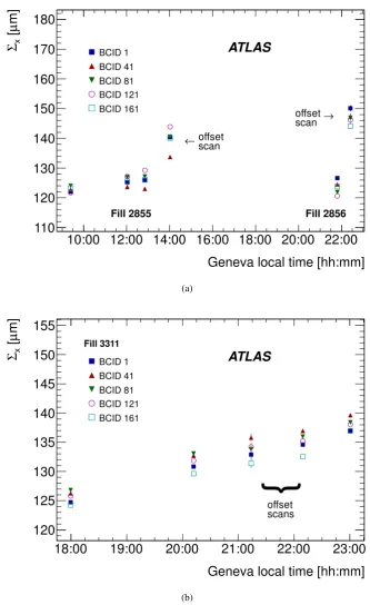
An unambiguous signature of non-factorization can be provided by comparing the transverse convolved width measured during centred (or on-axis)vdMscans with the same quantity extracted from an offset (or off-axis) scan, i.e. one where the two beams are significantly separated in the direction orthogonal to that of the scan. This is illustrated in Fig.3(a). The beams remained vertically centred on each other during the first three horizontal scans (the first horizontal scan) of LHC fill 2855 (fill 2856), and were separated vertically by approximately 340µm (roughly 4σb) during the last horizontal scan in each fill. In both

fills, the horizontal convolved beam size is significantly larger when the beams are vertically separated, demonstrating that the horizontal luminosity distribution depends on the vertical beam separation, i.e. that the horizontal and vertical luminosity distributions do not factorize.

this trend is observed when the beams are separated vertically, suggesting that the horizontal luminosity distribution is independent of the vertical beam separation, i.e. that during the November scan session the horizontal and vertical luminosity distributions approximately factorize.

4.8.2 Determination of single-beam parameters from luminous-region and luminosity-scan data

While a single off-axis scan can provide convincing evidence for non-factorization, it samples only one thin slice in the (δx, δy) beam-separation space and is therefore insufficient to fully determine the

two-dimensional luminosity distribution. Characterizing the latter by performing an x–ygrid scan (rather than two one-dimensional x andy scans) would be prohibitively expensive in terms of beam time, as well as limited by potential emittance-growth biases. The strategy, therefore, is to retain the standard vdM technique (which assumes factorization) as the baseline calibration method, and to use the data to constrain possible non-factorization biases. In the absence of input from beam–gas imaging (which requires a vertex-position resolution within the reach of LHCb only), the most powerful approach so far has been the modelling of the simultaneous beam-separation-dependence of the luminosity and of the luminous-region geometry. In this procedure, the parameters describing the transverse proton-density distribution of individual bunches are determined by fitting the evolution, duringvdMscans, not only of the luminosity itself but also of the position, orientation and shape of its spatial distribution, as reflected by that of reconstructedpp-collision vertices [23]. Luminosity profiles are then generated for simulated vdMscans using these fitted single-beam parameters, and analysed in the same fashion as realvdMscan data. The impact of non-factorization on the absolute luminosity scale is quantified by the ratioRNF of

the “measured” luminosity extracted from the one-dimensional simulated luminosity profiles using the standardvdMmethod, to the “true” luminosity from the computed four-dimensional (x, y, z, t) overlap integral [7] of the single-bunch distributions at zero beam separation. This technique is closely related to beam–beam imaging [7,24, 25], with the notable difference that it is much less sensitive to the vertex-position resolution because it is used only to estimate a small fractional correction to the overlap integral, rather than its full value.

The luminous region is modelled by a three-dimensional (3D) ellipsoid [7]. Its parameters are extracted, at each scan step, from an unbinned maximum-likelihood fit of a 3D Gaussian function to the spatial distribution of the reconstructed primary vertices that were collected, at the corresponding beam separa-tion, from the limited subset of colliding-bunch pairs monitored by the high-rate, dedicated ID-only data stream (Sect.3.2). The vertex-position resolution, which is somewhat larger (smaller) than the transverse luminous size during scan sets I–III (scan sets IV–XV), is determined from the data as part of the fit-ting procedure [23]. It potentially impacts the reported horizontal and vertical luminous sizes, but not the measured position, orientation nor length of the luminous ellipsoid.

The single-bunch proton-density distributionsρB(x, y,z) are parameterized, independently for each beam

B(B=1, 2), as the non-factorizable sum of up to three 3D Gaussian or super-Gaussian [26] distributions (Ga,Gb,Gc) with arbitrary widths and orientations [27,28]:

ρB=waB×GaB+(1−waB)[wbB×GbB+(1−wbB)×GcB],

where the weightswa(b)B, (1−wa(b)B) add up to one by construction. The overlap integral of these density

Geneva local time [hh:mm] 10:00 12:00 14:00 16:00 18:00 20:00 22:00

m]

µ

[_x

Σ

110 120 130 140 150 160 170 180

ATLAS

Fill 2855 Fill 2856

←_scanoffset

→ scan offset BCID 1

BCID 41 BCID 81 BCID 121 BCID 161

(a)

Geneva local time [hh:mm]

18:00 19:00 20:00 21:00 22:00 23:00

m]

µ

[_x

Σ

120 125 130 135 140 145 150 155

ATLAS

scans offset

{

Fill 3311

BCID 1 BCID 41 BCID 81 BCID 121 BCID 161

(b)

Figure 3: Time evolution of the horizontal convolved beam sizeΣxfor five different colliding-bunch pairs (BCIDs),

Horizontal beam separation [mm] 0.4

− −0.2 0 0.2 0.4

] -2 p) 11 [(10₂ n1 / n vis µ 0 0.01 0.02 0.03 0.04 0.05 0.06 0.07 0.08

LHC Fill 2855

Data (Centred x-scan IV July 2012)

Simulated profile of each beam: 3-D double Gaussian

ATLAS

(a)

Horizontal beam separation [mm] 0.4

− −0.2 0 0.2 0.4

Horizontal luminous centroid position [mm]

0.02 − 0.01 − 0 0.01 0.02 0.03

LHC Fill 2855

Data (Centred x-scan IV July 2012)

Simulated profile of each beam: 3-D double Gaussian ATLAS

(b)

Horizontal beam separation [mm] 0.4

− −0.2 0 0.2 0.4

Horizontal luminous width [mm]

0.06 0.07 0.08 0.09

0.1 _{LHC Fill 2855}Data (Centred x-scan IV July 2012)

Simulated profile of each beam: 3-D double Gaussian ATLAS

(c)

Horizontal beam separation [mm] 0.4

− −0.2 0 0.2 0.4

Vertical luminous width [mm]

0.06 0.07 0.08 0.09

0.1 _{LHC Fill 2855}Data (Centred x-scan IV July 2012)

Simulated profile of each beam: 3-D double Gaussian ATLAS

(d)

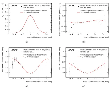
Figure 4: Beam-separation dependence of the luminosity and of a subset of luminous-region parameters during horizontalvdMscan IV. The points represent (a) the specific visible interaction rate (or equivalently the specific luminosity), (b) the horizontal position of the luminous centroid, (c) and (d) the horizontal and vertical luminous widthsσxLandσyL. The red line is the result of the fit described in the text.

orbit drifts and beam–beam corrections. The bunch parameters are then adjusted, by means of aχ2 -minimization procedure, to provide the best possible description of the centroid position, the orientation and the resolution-corrected widths of the luminous region measured at each step of a given set of on-axis x andyscans. Such a fit is illustrated in Fig.4for one of the horizontal scans in the July 2012 session. The goodness of fit is satisfactory (χ2 = 1.3 per degree of freedom), even if some systematic deviations are apparent in the tails of the scan. The strong horizontal-separation dependence of the vertical luminous size (Fig.4(d)) confirms the presence of significant non-factorization effects, as already established from the off-axis luminosity data for that scan session (Fig.3(a)).

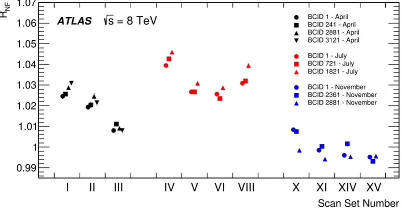
Scan Set Number

NF

R

0.99 1 1.01 1.02 1.03 1.04 1.05 1.06 1.07

I II III IV V VI VIII X XI XIV XV

BCID 1 - April BCID 241 - April BCID 2881 - April BCID 3121 - April BCID 1 - July BCID 721 - July BCID 1821 - July BCID 1 - November BCID 2361 - November BCID 2881 - November

ATLAS _{s = 8 TeV}

Figure 5: RatioRNFof the luminosity determined by thevdMmethod assuming factorization, to that evaluated from

the overlap integral of the reconstructed single-bunch profiles at the peak of each scan set. The results are colour-coded by scan session. Each point corresponds to one colliding-bunch pair in the dedicated ID-only stream. The statistical errors are smaller than the symbols.

in the LHC injector chain [16]. These observations are consistent, in terms both of absolute magnitude and of time evolution within a scan session, with those reported by LHCb [21] and CMS [29,30] in the same fills.

4.8.3 Non-factorizablevdMfits to luminosity-scan data

A second approach, which does not use luminous-region data, performs a combined fit of the measured beam-separation dependence of the specific visible interaction rate to horizontal- and vertical-scan data simultaneously, in order to determine the overlap integral(s) defined by either Eq. (8) or Eq. (10). Con-sidered fit functions include factorizable or non-factorizable combinations of two-dimensional Gaussian or other functions (super-Gaussian, Gaussian times polynomial) where the (non-)factorizability between the two scan directions is imposed by construction.

The fractional difference betweenσvis values extracted from such factorizable and non-factorizable fits,

i.e. the multiplicative correction factor to be applied to visible cross-sections extracted from a standard vdManalysis, is consistent with the equivalent ratioRNFextracted from the analysis of Sect.4.8.2within

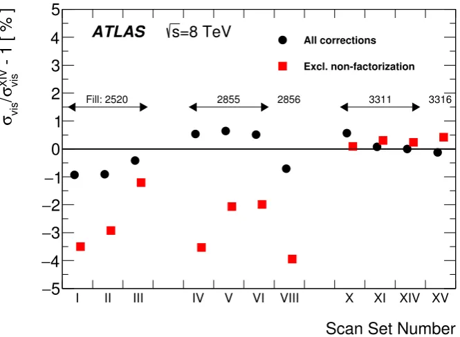
Scan Set Number

I II III IV V VI VIII X XI XIV XV

- 1 [ % ]

XIV vis

σ

/

vis

σ

5

−

4

−

3

−

2

−

1

−

0 1 2 3 4 5

All corrections

Excl. non-factorization

ATLAS _{s=8 TeV}

Fill: 2520 2855 2856 3311 3316

Figure 6: Comparison ofvdM-calibrated visible cross-sections for the default track-counting algorithm, with all corrections applied (black circles) and with all corrections except for non-factorization (red squares). Shown is the fractional difference between the visible cross-section from a given scan set, and the fully corrected visible cross-section from scan set XIV. The LHC fill numbers corresponding to each scan set are indicated.

4.8.4 Non-factorization corrections and scan-to-scan consistency

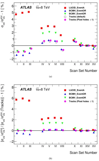
Non-factorization corrections significantly improve the reproducibility of the calibration results (Fig.6). Within a given LHC fill and in the absence of non-factorization corrections, the visible cross-section increases with time, as also observed at other IPs in the same fills [21,29], suggesting that the underlying non-linear correlations evolve over time. Applying the non-factorization corrections extracted from the luminous-region analysis dramatically improves the scan-to-scan consistency within the April and July scan sessions, as well as from one session to the next. The 1.0–1.4% inconsistency between the fully corrected cross-sections (black circles) in scan sets I–III and in later scans, as well as the difference between fills 2855 and 2856 in the July session, are discussed in Sect.4.11.

4.9 Emittance-growth correction

ThevdM scan formalism assumes that both convolved beam sizes Σx, Σy (and therefore the transverse

emittances of each beam) remain constant, both during a single xoryscan and in the interval between the horizontal scan and the associated vertical scan.

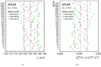
m] µ [

x

Σ

105 110 115 120 125 130 135 140 145

BCID 1 41 81 121 161 201 241 721 761 801 841 881 921 961 1581 1621 1661 1701 1741 1781 1821 2161 2201 2241 2281 2321 2361 2401 2881 BCMH_EventOR Scan set XI Scan set XIV Scan set XV

ATLAS

= 8 TeV s (a) ] -2 p) 11 ) [(10 2 n 1 /(n vis MAX µ

0.035 0.045 0.055

BCID 1 41 81 121 161 201 241 721 761 801 841 881 921 961 1581 1621 1661 1701 1741 1781 1821 2161 2201 2241 2281 2321 2361 2401 2881 BCMH_EventOR Scan set XI Scan set XIV Scan set XV

ATLAS

= 8 TeV s

(b)

Figure 7: Bunch-by-bunch (a) horizontal convolved beam size and (b) peak specific interaction rate measured in scan sets XI, XIV, and XV for the BCMH_EventOR algorithm. The vertical lines represent the weighted average over colliding-bunch pairs for each scan set separately. The error bars are statistical only, and are approximately the size of the marker.

Emittance growth between scans manifests itself by a slight increase of the measured value ofΣfrom one scan to the next, and by a simultaneous decrease in specific luminosity. Each scan set requires 40 to 60 minutes, during which time the convolved beam sizes each grow by 1–2%, and the peak specific interaction rate decreases accordingly as 1/(ΣxΣy). This is illustrated in Fig7, which displays theΣxand

µMAX

vis /(n1n2) values measured by the BCMH_EventOR algorithm during scan sets XI, XIV and XV. For

each BCID, the convolved beam sizes increase, and the peak specific interaction rate decreases, from scan XI to scan XIV; since scan XV took place very early in the following fill, the corresponding transverse beam sizes (specific rates) are smaller (larger) than for the previous scan sets.

If the horizontal and vertical emittances grow at identical rates, the procedure described in Sect. 4.3

remains valid without any need for correction, provided the decrease in peak rate is fully accounted for by the increase in (ΣxΣy), and that the peak specific interaction rate in Eq. (11) is computed as the average

of the specific rates at the peak of the horizontal and the vertical scan:

µMAX

vis /n1n2 =

(µMAX_vis /n1n2)x + (µMAX_vis /n1n2)y

2 .

width grew 1.5–2 times faster than the vertical width. The potential bias associated with unequal hori-zontal and vertical growth rates can be corrected for by interpolating the measured values ofΣx,Σyand

µMAX

vis to a common reference time, assuming that all three observables evolve linearly with time. This

reference time is in principle arbitrary: it can be, for instance, the peak of thexscan (in which case only

Σyneeds to be interpolated), or the peak of theyscan, or any other value. The visible cross-section, com-puted from Eq. (11) using measured values projected to a common reference time, should be independent of the reference time chosen.

Applying this procedure to the November scan session results in fractional corrections toσvisof 1.38%,

0.22% and 0.04% for scan sets X, XI and XIV, respectively. The correction for scan set X is exception-ally large because operational difficulties forced an abnormally long delay (almost two hours) between the horizontal scan and the vertical scan, exacerbating the impact of the unequal horizontal and vertical growth rates; its magnitude is validated by the noticeable improvement it brings to the scan-to-scan re-producibility ofσvis.

No correction is available for scan set XV, as no other scans were performed in LHC fill 3316. However, in that case the delay between thexandyscans was short enough, and the consistency of the resulting

σvisvalues with those in scan sets XI and XIV sufficiently good (Fig.6), that this missing correction is

small enough to be covered by the systematic uncertainties discussed in Sects.5.2.6and5.2.8.

Applying the same procedure to the July scan session yields emittance-growth corrections below 0.3% in all cases. However, the above-described correction procedure is, strictly speaking, applicable only when non-factorization effects are small enough to be neglected. When the factorization hypothesis no longer holds, the very concept of separating horizontal and vertical emittance growth is ill-defined. In addition, the time evolution of the fitted one-dimensional convolved widths and of the associated peak specific rates is presumably more influenced by the progressive dilution, over time, of the non-factorization effects discussed in Sect.4.8above. Therefore, and given that the non-factorization corrections applied to scan sets I-VIII (Fig.5) are up to ten times larger than a typical emittance-growth correction, no such correction is applied to the April and July scan results; an appropriately conservative systematic uncertainty must be assigned instead.

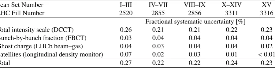
4.10 Bunch-population determination

The bunch-population measurements are performed by the LHC Bunch-Current Normalization Working Group and have been described in detail in Refs. [21,27, 31–33]. A brief summary of the analysis is presented here. The fractional uncertainties affecting the bunch-population product (n1n2) are

summar-ized in Table4.

Scan Set Number I–III IV–VII VIII–IX X–XIV XV

LHC Fill Number 2520 2855 2856 3311 3316

Fractional systematic uncertainty [%]

Total intensity scale (DCCT) 0.26 0.21 0.21 0.22 0.23

Bunch-by-bunch fraction (FBCT) 0.03 0.04 0.04 0.04 0.04

Ghost charge (LHCb beam–gas) 0.04 0.03 0.04 0.04 0.02

Satellites (longitudinal density monitor) 0.07 0.02 0.03 0.01 <0.01

Total 0.27 0.22 0.22 0.24 0.23

Table 4: Systematic uncertainties affecting the bunch-population productn1n2during the 2012vdMscans.

A precision current source with a relative accuracy of 0.05% is used to calibrate the DCCT at regular intervals. An exhaustive analysis of the various sources of systematic uncertainty in the absolute scale of the DCCT, including in particular residual non-linearities, long-term stability and dependence on beam conditions, is documented in Ref. [31]. In practice, the uncertainty depends on the beam intensity and the acquisition conditions, and must be evaluated on a fill-by-fill basis; it typically translates into a 0.2–0.3% uncertainty in the absolute luminosity scale.

Because of the highly demanding bandwidth specifications dictated by single-bunch current measure-ments, the FBCT response is potentially sensitive to the frequency spectrum radiated by the circulating bunches, timing adjustments with respect to the RF phase, and bunch-to-bunch intensity or length vari-ations. Dedicated laboratory measurements and beam experiments, comparisons with the response of other bunch-aware beam instrumentation (such as the ATLAS beam pick-up timing system), as well as the imposition of constraints on the bunch-to-bunch consistency of the measured visible cross-sections, resulted in a<0.04% systematic luminosity-calibration uncertainty in the luminosity scale arising from the relative-intensity measurements [27,32].

Additional corrections to the bunch-by-bunch population are made to correct forghost chargeand satel-lite bunches. Ghost charge refers to protons that are present in nominally empty bunch slots at a level below the FBCT threshold (and hence invisible), but which still contribute to the current measured by the more accurate DCCT. Highly precise measurements of these tiny currents (normally at most a few per mille of the total intensity) have been achieved [27] by comparing the number of beam–gas vertices reconstructed by LHCb in nominally empty bunch slots, to that in non-colliding bunches whose cur-rent is easily measurable. For the 2012 luminosity-calibration fills, the ghost-charge correction to the bunch-population product ranges from −0.21% to −0.65%; its systematic uncertainty is dominated by that affecting the LHCb trigger efficiency for beam–gas events.