Performance prediction for sailing dinghies

Performance Prediction for Sailing Dinghies

Prof Alexander H Day

Department of Naval Architecture, Ocean and Marine Engineering

University of Strathclyde

Henry Dyer Building

100 Montrose St

Glasgow G4 0LZ

[email protected]

Abstract

This study describes the development of an approach for performance prediction for a sailing dinghy. Key modelling issues addressed include sail depowering for sailing dinghies which cannot reef; effect of crew physique on sailing performance, components of hydrodynamic and aerodynamic drag, decoupling of heel angle from heeling moment, and the importance of yaw moment equilibrium.

In order to illustrate the approaches described, a customised velocity prediction program (VPP) is developed for a Laser dinghy. Results show excellent agreement with measured data for upwind sailing, and correctly predict some phenomena observed in practice. Some discrepancies are found in downwind conditions, but it is speculated that this may be related at least in part to the sailing conditions in which the measured data was gathered.

The effect of crew weight is studied by comparing time deltas for crews of different physique relative to a baseline 80kg sailor. Results show relatively high sensitivity of the performance around a race course to the weight of the crew, with a 10kg change contributing to time deltas of more than 60 seconds relative to the baseline sailor over a race of one hour duration at the extremes of the wind speed range examined.

Keywords

Performance Prediction for Sailing Dinghies

1

Introduction

1.1

Velocity Prediction Programs

Velocity Prediction Programs (VPPs) for sailing yachts were first developed more than thirty-five years ago (Kerwin (1978)) and a wide variety of commercial software is available. Whilst many commercial VPPs address generic displacement sailing yachts, customised VPPs have also been written for a wide variety of vessels from classic yachts (Oliver and Robinson (2008)) to high performance hydrofoil dinghies (e.g. Findlay & Turnock (2008)). Conventional VPPs aim at calculating steady-state solutions for boat speed and attitude over a range of true wind speeds and directions; however some attention has also been focussed on time-domain solutions which can better address performance in waves, through manoeuvres, and with unsteady wind speed (e.g. Harris et. al. (2001), Day et al. (2002), Verwerft and Keuning (2008))

1.2

Velocity Prediction Programs for Sailing Dinghies

For a sailing dinghy of moderate performance the basic framework for a VPP is broadly similar to that for a sailing yacht, but there are several key differences. Unlike yachts, sailing dinghies do not generally reduce sail size (or reef) in stronger winds. Hence approaches used in “standard” VPPs to reflect the reduction in sail area by reefing are not appropriate, and the models used to reflect the impact of depowering should reflect this. Furthermore, the impact of crew weight on stability is relatively small for a displacement yacht, and as a first approximation, the heel angle for a given heeling moment is essentially linked directly to the righting moment via the GZ curve. In contrast for a modern sailing dinghy, crew weight can contribute more than 50% of the total weight; the crew can move around the boat, altering the heel and trim angles of the hull substantially. Whilst the maximum righting moment generated by the crew is ultimately limited by the size and weight of the crew and the positions which can be adopted during sailing, the freedom of the crew to move around the boat essentially decouples the heel angle from the available righting moment, and hence the boat can be sailed at a range of heel angles.

A more minor difference for sailing dinghies compared to yachts is that dinghies generally race around relatively simple and well-defined courses; hence the definition of complete speed polars defining the relationship between the boat speed and the angle sailed to true wind is not required. In many cases, windward-leeward courses are adopted in which only two legs are sailed – one directly upwind and one directly downwind. In these cases, naturally, only the maximum upwind and downwind velocities made good (VMGs) are of interest.

common supplier. Hence there is no scope for design improvement in the boat. However there are still avenues for exploration of performance changes via changes in the crew physique, particularly in the crew weight; for example if the weather statistics are known for a particular venue, the crew weight may be optimised to maximise the speed around a race course.

1.3

Velocity Prediction Programs for the

Laser

Dinghy

Binns et al. (2002) describe the development of a (physical) sailing simulator based on a Laser dinghy. This utilised an unsteady VPP, which included the equations of equilibrium for longitudinal and side forces as well as heel and yaw moments. The upright resistance was based on the Delft series regression equations (Gerritsma et al. (1993)), while the lift and drag forces from dagger board and rudder were estimated using coefficients from Lewis (1989). This VPP also utilised the sail coefficients from Marchaj (1979) of the aerodynamics of Finn dinghy sails, with corrections made to them to account for aspect ratio effects. The VPP also included a number of models for the dynamics of the boat in manoeuvres, including the assessment of static and dynamic cross-coupling effects, the impact of sheeting angle, rudder dynamics (sculling), gusts, and time dependent lift build-up. Results are given in the form of speed polars for 9 and 12 knots wind speed.

angle of attack of the sail, rather than the heading of the boat, so an additional step is required in the VPP to estimate the sail trim at different headings, which is not explained.

The VPP solved for longitudinal, transverse, and heel equilibrium; however it was assumed that the boat remained upright in all conditions, based on argument that this gives the fastest performance. This is approximately true for upwind sailing, but is certainly not true when sailing downwind in light winds (see section 6.3). Heel equilibrium in the upright condition was achieved by adjusting the sail depowering variables. The programme allowed for sailors of different height and weight, at least for stability purposes, but the detail of the approach adopted to address this was not explained. Some anomalies were identified in regard to stability, including a lightweight (150lb) sailor out performing a heavyweight (210lb) in strong wind conditions, apparently due to a failure to maintain heel moment equilibrium. The results generally appeared somewhat noisy, with one or two unexpected deviations. Results from these two studies are discussed in section 6.2.

1.4

Current Study: The

Laser

Dinghy

The current study addresses the key differences between performance prediction for sailing dinghies compared to yachts, including the effects of depowering and the importance of crew weight. A customised VPP is then developed for a Laser dinghy, and the results are used to quantify the sensitivity of the performance of the boat to crew weight, enabling the identification of the optimum crew weight for the boat to be chosen for a given wind condition to maximise the speed around a simple windward-leeward race course.

2

Aerodynamic model for sailing dinghies

2.1

Background

Aerodynamic models in VPPs are often based on data taken from the Offshore Racing Congress (formerly IMS) VPP (Offshore Rating Congress (2013) section 5). This data consists of sets of baseline lift and drag coefficients tabulated at discrete apparent wind angles for fully powered-up sails. The interpolation for apparent wind angles between these points is carried out using a cubic spline. Two sets of data are quoted reflecting the difference between “simple” rigs with limited control on mast bend (and hence sail shape), which use the “low lift” coefficients, and more complex rigs which deploy additional rigging such as inner forestays or check stays to give greater control over mast bend and hence sail shape.

The majority of sailing dinghies have relatively simple fractional rigs, with limited control on mast bend, while some single sail boats such as the Laser have unstayed masts, and hence it seems appropriate to use the low lift coefficients, especially for dinghies without “fully-battened” rigs. However, since these coefficients are derived from wind tunnel tests of sailing yachts rather than dinghies, some further confirmation of the validity of the data in the current context is desirable.

Tests were carried out in turbulent and “smooth” flow. The tests were carried out at a range of heel angles from 0-30 degrees; the apparent wind resolved in the plane of the deck varied from around 26 degrees to 30 degrees in the upwind case.

The lift coefficients quoted in the upwind condition peaked around 1.53 in turbulent flow at an apparent wind angle in the deck plane of around 28.5 degrees. In smooth flow, the value at the same angle was 1.61. These lift coefficients appear rather high in comparison with those of Table 1. However the sail area used as a reference for the calculation of the coefficients is the “triangular” area based on the luff and foot lengths. In contrast, the sail area used in conjunction with the ORC coefficients is the cloth area calculated according to the ORC formula, with a correction for additional area due to the foot curve. Correcting for this difference in area reduces the Laser sail lift coefficients in smooth and turbulent flow from Flay’s study respectively to 1.30 and 1.36. The value in the ORC table for “low lift” mainsail coefficients at an angle of 28 degrees is 1.347, which falls between these two values, suggesting that the ORC “low lift” coefficients are appropriate for a Laser, at least for upwind sailing. The full set of coefficients is given in Table 1.

The drag coefficients given by Flay (loc.cit.) relate to the total aerodynamic drag, including the effects of the spars and hull (no model crew was used). The total drag coefficient measured in the wind tunnel in turbulent flow, corrected to the cloth area of the sail, was around 0.27. It can be seen from Table 1 that little of this drag can be expected to result from the viscous drag of the sail, with the majority coming from induced drag and parasitic drag of hull and spars. In comparison, at this angle of attack, with 10 degrees of heel (corresponding to the wind tunnel tests) the predicted total drag coefficient based on the ORC coefficients and approach to parasitic drag calculation (excluding the crew) is 0.20. It is difficult to explain this discrepancy; however given that only a very small data set is available from these tests, the ORC approach is adopted here.

position (required for the yaw balance calculation) is assumed to be 33% of the foot length aft of the luff. It should be noted that the Laser exhibits significant mast bend when sailing upwind which has the effect of moving the CE further aft than if the mast were straight. Analysis of photographs of Lasers sailing upwind indicates a typical equivalent mast rake at the CE height of 11 degrees; this

value is utilised in the yaw moment calculation in the upwind condition.

2.2

Depowering models for sailing dinghies

In stronger winds, when boat speed becomes limited by the available righting moment, sailors depower the sails to reduce heeling moment and thus heel angle. By reducing the lift and/or heeling lever, the heel angle is reduced and the impact of reduced hull resistance is traded off against the reduction in drive. In the case of sailing dinghies which generally cannot reef (i.e. reduce sail area), the modelling of this depowering process is particularly important when considering the impact of crew weight on performance.

2.3

REEF, FLAT and TWIST

In VPPs, depowering is normally addressed by modifying sail coefficients using a semi-empirical depowering model. A commonly adopted approach in simple yacht VPPs, as proposed originally by Kerwin (1978), utilises the non-dimensional REEF and FLAT coefficients. These effect a rather idealised representation of the physical processes of reefing and flattening sails, affecting lift, drag and heeling moment from the sailplan. The fully powered up lift and drag coefficients are described as:

(1)

( )

( )

( )

( )

(

)

max

2 max 1

L L

D Dv Dp L E Ds

C C

C C C C AR C

β β

β β p

′ = ′

′ = ′ + + +

Here CLmaxis the fully-powered lift coefficient at the apparent wind angle

β

Dv

mast, crew etc. The final term in the drag equation is the lift-related drag 2

(

)

max 1

L E Ds

C pAR +C .

Here the first term in the bracket is the induced drag based on the standard result from lifting line

theory, using an effective aspect ratio ARE. The second term CDsis the separation drag coefficient

reflecting the increase in viscous pressure drag with lift in 2D flow due to boundary layer thickening.

max

L

C and C_Dv are obtained by interpolation from tabulated values varying with apparent wind

angle, while CDsis typically treated as a constant, taken here as 0.005. The effective aspect ratio

E

AR is calculated from the geometric aspect ratio based on rig geometry modified using empirical

coefficients. These coefficients are modified by the REEF and FLAT coefficients r and

f

(2)

(

)

( )

(

)

(

( )

(

)

)

* 2

max

* 2 2 2

max , , . .

, , . 1

L L

D Dv Dp L E Ds

C r f f r C

C r f r C C f C AR C

β β

β β p

′ = ′

′ = ′ + + +

where *

L

C and *

D

C are the depowered lift and drag coefficients. The effect of FLAT is to reduce the

lift coefficient without affecting viscous drag. This corresponds loosely to the impact of flattening the sails. The solution algorithm for a simple VPP for a displacement yacht typically adjusts the

depowering parameters rand

f

equilibrium. Vertical equilibrium can be considered to be satisfied by default for a displacement vessel. Whilst this model has been remarkably successful, and has been used for many years a number of limitations have become increasingly obvious. One limitation of this model is that it implicitly assumes that the coefficient linking the lift-related drag to the square of the lift remains independent of REEF and FLAT via the relation:

(3) Di₂ 1 or Di₂

Ds

L E L

C C

C k

C pAR C

 

=_ + _ =

 

are sailing upwind in moderate wind conditions, in which heel is not a limiting factor, the sails will typically be trimmed to generate maximum drive. In these conditions, wind tunnel tests suggest that some flow separation is present (Fossati et al. (2006)), and hence the drag in this condition is higher than suggested by the calculation. As the wind speed increases sailors typically reduce heeling moment when sailing upwind by increasing the twist of the sails before reefing. Adjusting the sails to generate more twist than the optimum value reduces the heeling moment by selectively depowering the upper part of the sail; however it simultaneously increases the induced drag coefficient (Hansen et. al. (2006)).

A more refined approach, originally proposed by Jackson (1996, 2001), and developed further by authors such as Hansen et al. (2006), introduces a TWIST coefficient. The idea of this coefficient is that the distribution of lift is modified so that less lift is generated higher in the sail and more lift is generated lower in the sail so that the total lift generated by the sail remains unchanged. This coefficient may be used in addition to REEF; however in the current study, since dinghies do not reef, TWIST is used in place of REEF. Using the TWIST model for a single sail boat the height of the centre of effort above the boom is calculated as:

(4) *

(

)

. 1

CE b CE b

Z =Z −t

(5)

(

)

( )

(

)

( )

( )

* 2 2

max , , . 1 . , , . L L twist

D Dv Dp L Ds

E

C t f f C

C t

C t f C C f C C

AR

β β

β β β

p

′ = ′

 + 

′ = ′ + + ′ _ + _

 

The value of Ctwist is taken here as 8.0, following Jackson (2001). Increasing twist thus has a net

effect similar to reducing the effective aspect ratio. This approach to twist is rather different from that adopted in the 2013 ORC VPP (Offshore Racing Council (2013)) for a sloop-rigged yacht, which corrects the centre of effort height in relation to the FLAT parameter as well as the “fractionality” of the rig, but neglects the impact of twist on induced drag.

2.4

Other Approaches

Many dinghies sail upwind with apparent wind angles close to the point at which lift coefficient is maximum. For angles of apparent wind from zero up to the point of maximum lift (around 34 degrees), it is likely that the mainsail sheeting angle relative to the boat for maximum lift will not change. For a single-sail dinghy sailing near to the angle of maximum lift coefficient the effect of spilling wind without adjusting the sail twist is equivalent to simply reducing the apparent wind angle on the sail as there are no sail interaction effects to consider. Thus over this range of apparent wind angles, if the sail angle is reduced by 10 degrees say, the impact on lift and drag could then be modelled by simply recalculating the sail coefficients for an apparent wind angle reduced by 10 degrees. For a sloop-rigged dinghy, a similar approach could be applied to the mainsail but not the headsails, since the headsail cannot typically be eased without affecting twist.

Table 1 shows that a reduction in the apparent wind angle from a point close to the maximum lift will lead to a small reduction in the drag coefficient between 28.0 and 12.0 degrees before a small rise is seen between 12.0 and 0.0 degrees.

In the current study therefore a further approach is examined by introducing a variable SPILL for upwind sailing only which reduces the angle of attack for which the sail coefficients are calculated. SPILL is constrained to lie between zero and the actual apparent wind angle, and is used in conjunction with FLAT and TWIST. In this model the equations are thus:

(6)

(

)

(

)

(

)

(

)

(

)

* 2 2

max , , , . 1 . , , , . L L twist

D Dv Dp L Ds

E

C t f s f C s

C t

C t f s C s C f C s C

AR

β β

β β β

p

′ = ′−

 + 

′ = ′− + + ′− _ + _

 

where s is the SPILL variable.

2.5

Parasitic Aerodynamic Drag

and the crew. The drag area of the mast, rigging, and topsides can be estimated following an approach similar to that set out in the 2013 ORC VPP (Offshore Racing Council (2013)).

For the purposes of estimating drag in the upwind condition, the mast is divided into the “bare” part and the part inside the sail sleeve. The bare part is assumed to have a drag coefficient of 0.8 and the part to which the sail is attached has corresponding coefficient of 0.15, based on results from Hoerner (1965) for thick fairings. The centre of pressure of each part is assumed to be at its midpoint. In the downwind condition, the sail sleeve and the mast is assumed to act as part of the sail with the same drag coefficient.

The topsides of the hull can be assumed to have a frontal area equal to the freeboard multiplied by the overall beam, and a side area equal to the freeboard multiplied by the overall length. A further correction is applied to allow for the heel of the boat, based on the mean beam estimated from the waterplane area coefficient. The projected area for different apparent wind angles is estimated using a sinusoidal function varying between these values. The key equations are presented below:

(7)

(

)

( )

(

)

(

)

. 0.5 . .sin .sin 0.66. 0.5 . .sin F Hull OA

S Hull OA OA WP

Hull F Hull S Hull F Hull

CE Hull OA WP

A B FA

A L FA B C

A A A A

Z FA B C

φ β β φ = = + = + − = +

Here AF Hull, is the frontal area of the topsides of the hull, BOA is the overall beam, FA is the average

freeboard. AS Hull, is the side area of the heeled topsides of the hull, LOA is the overall length, CWPis

the waterplane coefficient, φ is the heel angle. Finally βis the apparent wind angle, and ZCE Hull, is

the height of the centre of pressure of the aerodynamic drag on the topsides.

generated is specific to the body position adopted for these sports; similar studies have not been found by the author for sailing dinghies. Hence the aerodynamic drag of the crew is estimated here using data derived from wind tunnel studies for other purposes.

The surface area of a (nude) human can be estimated according to the formula of Dubois & Dubois (1916) as:

(8) ADu =0.0769W0.425H0.725

Where ADuis the estimated Dubois surface area in square metres, Wis the weight of the person in

Newtons and His the height in metres.

Penwarden et al. (1978) carried out measurements of frontal and sideways area and the drag coefficients of 331 people visiting a wind tunnel on an open day. The areas were related to the Dubois formula with a simple multiplier; the mean values were given as:

(9)

, ,

0.326

0.219

F crew Du

S crew Du

A A

A A

= =

A shielding factor is then applied to account for the shielding of part of the body by the cockpit, or in two-person dinghies, by the other crew member. In the present study, the drag area is reduced by 20% to account for shielding from the cockpit.

3

Hydrodynamic model for sailing dinghies

3.1

Introduction

The hydrodynamic model in simple VPPs is very often based on the Delft series formulation (e.g. Gerritsma et al. (1981), Keuning et al. (1996), Keuning & Katgert (2008)). The model comprises a series of polynomial regression equations derived from tank tests of over fifty sailing yacht models with varying speed, heel and leeway angle. This model may be modified (as it is here) to take advantage of measured data where available.

The Delft series model, as implemented in many generic VPPs, may need to be modified or replaced in order to address particular types of vessels. The hulls tested in the development of the model were all round-bilge sailing yacht forms with principal parameters reflecting yacht design practice during the many years of testing. Hence where hulls have principal form parameters falling outside the range of hulls tested in the generation of the Delft data set, the results may not be reliable. Equally, hulls which exhibit fundamental differences in shape not captured by form parameters (such as hard chine forms) may not be well represented, while sailing vessels completely dissimilar in terms of hydrodynamics to displacement yachts, such as catamarans and hydrofoil vessels, require a different approach (see for example Findlay & Turnock (2008)). Finally issues arise for high speed planing vessels for which the range of Froude Numbers in the Delft series model may not be adequate.

calculated for a set of hull forms. The meta-model can take the form of polynomial-type equations (such as those used in the Delft series) or may adopt more sophisticated modelling techniques such as Artificial Neural Networks (see for example Mason (2010)).

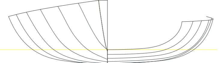
A further possibility relevant here is to utilise data obtained directly from hydrodynamic testing. Day & Nixon (2014) investigated the resistance of a Laser dinghy, using a hull model measured using an optical measurement system. The hull form generated is shown in Figure 1 with waterline shown for an all up mass of 160kg, based on a nominal mass for the hull foils and rig of 80kg and an 80kg crew. The hull is broadly similar to some of the yachts tested in the Delft series, whilst the form parameters shown in Table 2 for three displacements varying from 150-170kg lie well within the Delft range.

Model tests on the hull in the upright condition with no appendages under normal trim angles (with transom just touching static waterline for each displacement) showed broadly reasonable agreement with the Delft model for residuary resistance (Keuning & Katgert (2008), (equation 1)):

(10)

2 3 1 3 1 3

0 1 2 3 4 5 6 7

fpp fpp

rc c c wl wl c

p m

c wl w wl wl fpp c wl

LCB LCB

R B B

a a a C a a a a a C

g L A L L LCF T L

r

 

 ∇  ∇ ∇

= + ⋅ + ⋅ + ⋅ ⋅ +_ ⋅ + ⋅ + ⋅ + ⋅ _⋅

∇ ⋅ _{   }

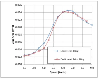
However it can be seen from the comparison between the prediction and the measurements shown in Figure 2 for a displacement of 160kg that the equation under-predicts the upright resistance in the critical 3-5 knot speed range, typical of upwind sailing in a Laser, by as much as 8%.

3.2

Hydrodynamic resistance

For the current purposes, therefore, the data from the model tests was used directly to predict the upright resistance of a Laser in the developed VPP by interpolation (and in some cases extrapolation) for weight and speed. However this is not the whole solution, since model tests were only conducted in the upright condition without appendages, and hence results were not available for other components of resistance.

The Delft framework considers eight components of hydrodynamic resistance: frictional and residuary resistance for the upright hull, viscous and residuary resistance for the keel in the upright condition, change in frictional and residuary resistance of the hull due to heel, change in residuary resistance of the keel due to heel, and induced drag of the hull/keel combination. Added to this in the current case is the resistance associated with the use of the rudder.

3.3

Hydrodynamic side force and yaw moment

The model as described above provides the information required for the VPP to satisfy equilibrium in the horizontal plane and also in heel. However, the impact of yaw can also usefully be considered to quantify the effect of rudder angle on speed.

In order to satisfy yaw equilibrium, the hydrodynamic and aerodynamic yawing moments must be calculated, and the sum set to zero by varying the rudder angle. This in turn requires that the leeway angle of the hull is found. The yaw moment from the hull is calculated here according to the approach proposed by Keuning & Verwerft (2009). In this approach the side force generated by the underwater body is calculated first for the daggerboard and rudder as a function of the leeway angle

λ

(11) .

2 .

. .

1

. . .

2 eff k

L k

k hull keel eff k lat k

dC

L c c V A

d

a

a

r

=

Note that in this equation the original notation is used with subscript “k” to denote “keel”, but this should be taken here as referring to the daggerboard.

Here the lift slope is estimated as

(

)

. _{5.7 1.8 cos cos 4}

L k E E dC AR AR d

a

= _ + L L + _

 , with the

effective aspect ratio of the daggerboard given as

AR

=

2

b

/

c

which accounts for “lift carry-over” effects is given as c_hull = +1 1.80

(

)

influence coefficient is found as

c

= −

1 0.382

φ

φ

The angle of attack over the daggerboard is equal to the leeway angle when the boat is upright, but is affected by the heel of the boat, as the underwater body becomes progressively more asymmetric

is the zero-lift drift angle of the hull estimated as

λ

=

(

0.405

(

B

T

)

φ

)

to the daggerboard Veff k. is simply the boat speed. The rudder is treated in a similar manner:

(12) .

2 .

. .

1

. . .

2 eff r

L r

r hull keel eff r lat r

dC

L c c V A

d

a

a

r

=

The key difference from the daggerboard is that the effective angle of attack on the rudder is affected both by downwash from the daggerboard and by the rudder angle; thus

. 0

eff r r

a

λ λ δ

r

δ

90% of the boat speed: Veff r. =0.9Vb. The total lift of the daggerboard and rudder for a given leeway

angle and rudder angle is thus obtained from the sum of the two components given in equations (11) and (12).

The hydrodynamic yaw moment from the daggerboard and rudder can be easily calculated from the moments generated by the respective lift components. Following Keuning & Vermeulen (2003) the centres of pressure of the daggerboard and rudder are each assumed to be located on the quarter chord line of the foils at 43% of the total draft of each of the foils (i.e. the vertical distance from the waterline to the lower extent of the foil). However there is a further component of yaw moment generated by the hull, related to the so-called Munk moment. Keuning & Vermeulen suggest that this may be calculated as:

(13)

( ) ( )

2 2 2 2 . . . 2 wl wl L b L

N

p r λ

=

_∫

( )

( )

( )

C x = c x − c x + , where c_ysis the local sectional area coefficient. The resulting moment thus depends both on the displacement and the heel angle. In the present study the Munk moment was calculated from free-trim hydrostatics using equation (13) for three different displacements and five heel angles, and it was found that the moment could be accurately represented as:

(14) N =N₀(1 0.00966+ φ_deg+0.00134φ_deg2 )

With the upright value

N

=

0.0002164

∆ −

0.014572

∆

total hydrodynamic yawing moment for a given leeway angle and rudder angle thus consists of the sum of the three components described above.

3.4

Induced Resistance

The standard Delft model (Keuning & Katgert (2008)) provides a model for the induced resistance of the hull-keel-rudder combination and with a defined speed and heeling force:

(15)

(

)

2 2 2

2

1 2 3 4 0 1

1 . . 2 h i b E

c c wl

E n c F R V T

T T B

T

A A A A TR B B F

T T T T

p r =  _{ }    =_ ⋅ + ⋅_{ } + ⋅ + ⋅ _⋅ + ⋅    

The coefficients in this equation are tabulated for different heel angles. However this model equation is based on tests with zero rudder angle. As soon as the rudder angle is non-zero, the lift on the rudder will change, and since the effective aspect ratio of the rudder will be different to that of the whole underwater body, the total induced drag will also change. In the present study this is addressed as described below:

(16) C_Di =C_L2

p

The lift coefficients of the rudder with rudder central and with rudder angle are determined from

equation (12). The planform efficiency e for a tapered swept foil where AR_E = AR e. is determined

following Nita & Scholz (2012) as

(17) e=1 / 1

(

(

)

)

With ∆TR= −0.357+0.45 exp 0.0375

(

)

( )

0.0524 0.1500 0.1659 0.0706 0.0119

f TR = TR − TR + TR − TR+

Here the aspect ratio includes the image in the free surface. The heel of the boat can be considered

to be equivalent to dihedral, thus modifying this value by a factor equal to 2

cos

φ

The approach described above is used to estimate the lift and associated induced drag of the rudder both on the centreline and with the given rudder angle, thus allowing the lift and induced drag deltas due to rudder angle to be estimated. The delta in the lift caused by the rudder angle is subtracted from the heeling force before applying equation (15) to estimate the hull and keel induced drag, and the delta in the rudder induced drag is then added to the total resistance.

This model neglects the impact of waves, which will be significant in some sailing conditions, both through slowing the boat while sailing upwind, and through allowing opportunity for significant speed gains due to surfing when sailing downwind. This is discussed further in section 6.1.

4

Stability of a sailing dinghy

The hydrostatic stability of sailing dinghies is strongly dependent on the crew position, since the crew typically contributes more than 50% of the total weight. The approach adopted here is based on a calculation of the maximum available righting moment as a function of heel angle based on the height and weight of the crew.

The CG of both men and women standing upright is typically 55-57% of their height (Palmer (1944), Croskey (1922). In this study the more conservative figure of 55% is adopted. However the body position adopted by even the fittest athletes will be less straight than in the standing position due to the geometry of the side decks of the boat; hence the upper limit of righting moment will occur with a transverse offset of crew CG less than 55% of the crew height. In the present VPP it is assumed that the transverse location of the crew CG (relative to their feet) is located at a position which allows the optimum heel angle; however it is assumed that it can be no more than 95% of the CG height in the standing position from the centreline.

The maximum available righting (or heeling) moment is therefore based on the condition with the crew CG at 95% of height from the centreline, either to windward or leeward, and this maximum moment is used as one constraint to the optimisation.

The vertical position of the crew CG in this hiking position is likely to be the lowest value possible; this is estimated relative to the boat CG. The maximum righting moment available at a given heel angle is given as:

(18) RMMAX =WHullGZ

( )

φ

(

( )

φ δ

φ δ

φ

)

where GZ

( )

crew YCG

δ

δ

when the crew is hiking to the maximum hiking potential.

For the VPP developed here, the VCG of the boat was first measured on a swing; the mast and boom were in position, but due to height restrictions, the daggerboard was placed on the deck at the correct longitudinal position, and the rudder blade was horizontal. Since the measurement was executed outdoors, the sail was not rigged in order to avoid unwanted effects due to wind. The total weight of the boat without the sail was found to be 79.5 kg, and the CG was found to be 12cm above the deck at the forward end of the cockpit. The GZ curve was then calculated for the three displacement conditions listed in Table 2, with the CG of the total system assumed to be at the CG of the boat. An estimate was then made of the position of the crew CG relative to this point when fully extended. The maximum righting moment calculated from this data is used as a constraint in the VPP solver as described in Section 5.

5

Solution procedure

The Excel “solver” was then used to solve the problem to maximise VMG both upwind and downwind. The design variables used for optimisation were speed, heel angle, true wind angle, leeway, rudder angle, TWIST, FLAT, and SPILL. The optimal solution was found subject to the constraints:

1) Abs (Total Resistance – Total Drive) < 0.01N

2) Min Right moment < Heeling Moment < Max Right Moment

3) Abs (aerodynamic heeling force – hydrodynamic heeling force) < 0.01N

4) Abs (aerodynamic yawing moment – hydrodynamic yawing moment) <0.01Nm 5) 0.0 < TWIST < 1.0; 0.6 < FLAT < 1.0; 0.0 < SPILL < β

Longitudinal equilibrium is satisfied explicitly via the first constraint. The second constraint ensures that the solution found for heel, which yields the optimal heel angle (in the sense of maximising VMG) is achievable within the range of righting moment which can be generated by a sailor of the given height and weight. Transverse force equilibrium and the associated yaw moment equilibrium are satisfied explicitly through the third and fourth constraints whilst vertical equilibrium is satisfied by equating weight and buoyancy. Trim equilibrium is assumed to be achieved by the movement of the crew longitudinally in the boat. The FLAT value is limited to a lower bound of 0.6 as discussed in section 2.2. The daggerboard was assumed to be fully down whilst sailing upwind and 50% down when sailing downwind. The only exception to the constraints described above are for the case in which yaw balance was neglected in which the third and fourth constraints were not imposed, and transverse equilibrium was imposed implicitly by equating the hydrodynamic heeling force to the corresponding aerodynamic force in the calculation of hydrodynamic induced drag.

was run for both upwind and downwind VMG, allowing the assessment of performance in a given wind speed for a given crew physique around a typical windward-leeward racecourse.

6

Results

6.1

Validation and comparison with measured data and previous VPP studies

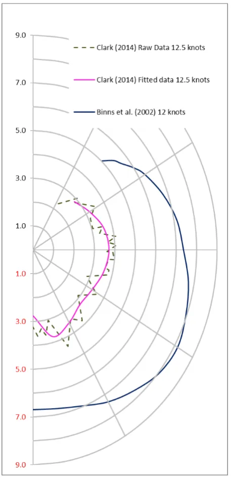
The results of the VPP may be validated by comparing with full-scale measurements. Two data sets are considered here. The first data set is presented by Binns et al. (2002), and was reported to have been made by one of the co-authors. The data is presented in the form of polar plots of speed against true wind angle for wind speeds of 9 and 12 knots. No information is given regarding the height and weight of the sailor or sailors, the instrumentation used for measuring speed, track, wind speed or angle measurements and its resulting uncertainty, or regarding the set-up or strategy adopting in sailing the boat whilst gathering data. The authors do comment that the measurements were made in conditions where some surfing downwind could be expected, which would lead to higher speeds than would be achieved in calm water, particularly in broad reaching conditions. The data set was extracted from the plots shown and is re-plotted here in Figure 3.

wake of the sailor and mast when sailing downwind, which would lead to potential for underestimating the wind speed.

Data was gathered as the boat was sailed around a triangular course; the windward and leeward marks were set so that one leg was approximately dead downwind; the wing mark was set so that the true wind on the other two legs was at approximately 45 degrees from the bow. The majority of the data collected was for upwind or dead downwind sailing with very little reaching. Dagger board position was not recorded. Speed polars were presented for all true wind angles based on the data gathered. The raw data yielded fairly noisy speed polars, and a processed version was presented, which was smoothed with a moving average filter. Both sets ere extracted from the presented plots and are shown in Figure 3. It appears that no attempt was made to discriminate between data gathered from steady-state sailing and that gathered during manoeuvres, hence it can be expected that some of the variations in speed with true wind angle may be caused by boat/sailor dynamics during manoeuvres (such as roll tacking and gybing). The wind speed presented was the average value obtained over the 11 laps, given as 12.53 knots; the lowest average windspeed was 10.68 knots, whilst the highest was 13.86 knots. The author comments that the wind was rather variable over the course due to the impact of surrounding buildings.

record. For these reasons, this data set is not considered further here, and comparisons are focussed on the first data set.

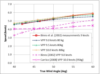
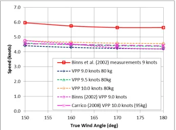
In this study, the primary focus is on maximising VMG upwind and downwind. The comparison between the present VPP with the experiment data and with the VPPs of Binns (2002) and Carrico (2005) for upwind sailing in winds of 9.0 knots is shown in Figure 4. Since the earlier studies do not give details of the sailor physique a baseline figure of height 1.8288m and weight of 80kg has been assumed for these calculations using the present VPP. This is often suggested as close to the optimum weight for a Laser over a range of conditions – for example, in a well-known guide to Laser sailing, Goodison (2008) (an Olympic Gold Medal winner in the Laser) suggests 78-83kg as optimum. The crew is assumed to be wearing 5kg of clothing, with clothing CG located at the crew CG.

A Laser can be expected to achieve maximum VMG upwind in true wind angles in the region around 40-46 degrees in flat water. Agreement for the current VPP in this key range of true wind angles can be seen to be good, particularly around 45 degrees. VPP results are plotted for 9.0, 9.5 and 10.0 knots; it can be seen that the boat speed is relatively insensitive to the wind speed over the range of angles up to about 50 degrees, which implies that the accuracy of the wind speed measurement is not critical at these headings. The sailor is just starting to depower very slightly at 9.0 knots when sailing upwind, and so increases in wind speed require further de-powering to maintain heel angle, reducing the opportunity to gain speed. The data shows more sensitivity to wind speed above 50 degrees, since the sail is fully powered up at 60 degrees (i.e. FLAT =1, TWIST = 0, SPILL = 0), and hence the increased available power in the wind can be exploited. It can be seen that the VPP of Binns et al. displays the correct trends, but under-predicts boat speed around the key wind angle by about a knot. The VPP of Carrico, with a heavier sailor, but in 10.0 knots of wind substantially under-predicts the speed; furthermore the VPP does not display the correct trend with wind angle.

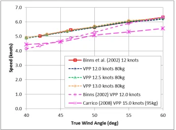
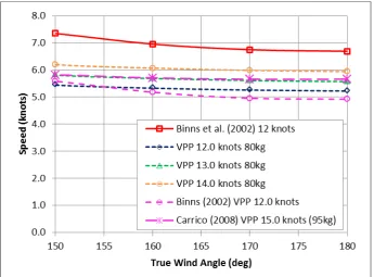
measured data over the range from 42 – 60 degrees, and showing very little sensitivity to wind speed as shown in Figure 5. In this region the sail is starting to be depowered throughout the range of upwind angles. The VPP results from Binns again show under prediction of speed in the 40-50 degree range, whilst the results of Carrico, for 15.0 knots, again under-predict the speed.

An approximate prediction of the additional speed due to surfing could be undertaken by a simplified approach such as that proposed by Harris et al. (2001), although that would require knowledge of wave conditions during the measurement programme.

In summary, it can be seen that the VPP correctly predicts the trends in measured speed data in both upwind and downwind conditions, and predicts upwind speed very accurately.

6.2

Results for baseline crew

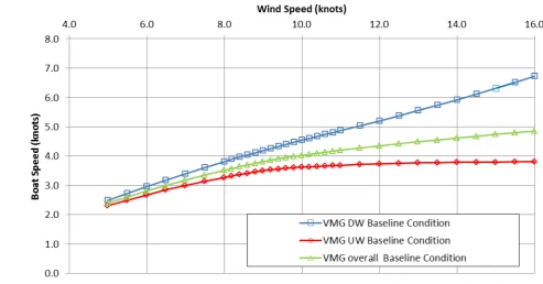
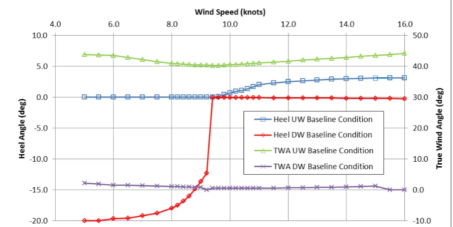
The overall VMG is calculated over a range of wind speeds by assuming a windward-leeward course with upwind and downwind legs of the same length. The times for each leg are calculated from the individual VMG values and added to give total lap time; the overall VMG is then simply the total lap length divided by total lap time. Results are shown in Figure 8, and corresponding heel and true wind angles are shown in Figure 9. Note that the downwind true wind angle is presented as the difference from 180 degrees.

The VPP results suggest that the optimum heel angle downwind is large negative for winds less than 9 knots, and then reduces in magnitude rapidly when the wind speed reaches around 9.5 knots. The explanation of this “mode shift” can be seen from Figure 10. Here the deltas due to frictional and residuary resistance are plotted against wind speed along with the heel angle. Note that the frictional resistance delta, which is negative, is plotted as positive for clarity. At 9 knots wind speed the penalty in residuary resistance of the hull is less than the benefit in frictional resistance due to reduced wetted area; however the penalty is increasing faster with wind speed. At 9.1 knots, it is still beneficial to have the boat heeled to windward, but by 9.15 knots the residuary resistance penalty exceeds the value of the frictional resistance penalty and a step change in heel angle results. It can be seen that the total delta due to heel varies smoothly.

known as “kiting”. Analysis of photographs of Lasers sailing downwind suggests that typical windward heel in light winds is around 20 degrees, and this is reflected in the heel angles seen in Figure 9. Goodison (2008) suggests kiting in light winds of 0-8 knots, but not in medium winds (8-16 knots); the VPP results are consistent with this.

The VPP predicts that the boat should be sailed flat upwind up to about 9 knots wind speed, and then at a small heel angle beyond that wind speed. The lowest true wind angle occurs at 9.5knots wind speed just as the sail is starting to be depowered. The apparent wind angle varies between around 27 degrees in 5 knots of wind up to around 33 degrees in 15 knots; all relatively close to the angle for which the sail generates maximum lift coefficient.

The percentage breakdown of the hull resistance components is shown for 5, 10 and 15 knot wind speeds in Figure 11. Here Ruh is the upright hull resistance, Rkvu is the viscous resistance of the daggerboard, Rkru is the residuary resistance of the daggerboard, Rrvu is the viscous resistance of the rudder, dRfh is the change in frictional resistance of the hull due to heel, dRrhphi is the change in residuary resistance of the hull due to heel, dRrkphi is the change in residuary resistance of the daggerboard due to heel, Ri is the induced resistance of hull and daggerboard, and dRi is the change in induced resistance due to the use of the rudder. The change in frictional drag of the hull due to heel is negative, so the total sums to 100%. It can be seen that upright hull resistance is dominant downwind, and less so upwind, for which induced drag becomes increasingly important as wind speed increases.

6.3

Yaw Balance

In order to examine the impact on the prediction of the boat performance of the inclusion of yaw balance, the runs described above were repeated without imposing yaw moment equilibrium; hence the boat was assumed to track in a straight line with the rudder central. The results in terms of boat speed are shown in Figure 13. It can be seen that including the yaw balance results in an increase in predicted upwind speed averaging around 1.0%. This may be expected; as suggested by Nomoto (1979) moderate weather helm can improve performance by differentially loading the rudder and unloading the hull/keel. Since the rudder is typically more efficient than the hull/keel combination this leads to a reduction in induced drag and increased speed. Downwind, there is very little impact, with an average drop in VMG due to the inclusion of yaw balance of less than 0.05%.

6.4

Impact of Sailor Physique

One of the primary goals of creating a VPP for a “one-design” sailing dinghy is to examine the effect of parameters which can be changed, such as crew physique, on performance. To this end, the VMGs for three sailors all of height 1.829m (6’ 0”), but with weights varying from 70-90kg are compared in Figure 15. As might be expected it can be seen that the lighter crew gains in all conditions downwind, and gains up to around 9.0 knots upwind, at which point the sail starts to become depowered. At that point the 90kg crew becomes fastest upwind.

The differences in speed are rather small, and in order to present the impact of these small speed changes in a meaningful manner, the results are also compared by calculating the difference in time taken over a windward-leeward course compared to a benchmark sailor who completes the course in one hour. In this calculation, no account is taken of time lost in manoeuvres or any tactical interactions between boats, nor the effects of waves or unsteady wind. Results showing the time deltas for eight sailors varying in height from 1.753m (5’9”) to 1.905 m (6’3”) and varying in weight from 70-90 kg are shown in Figure 16 for a range of true wind speeds from 5-15 knots.

In the light wind region the effect of crew height is small, with only a very small penalty for taller crews due to increased aerodynamic drag; the penalty for additional 10 kg weight is around 40s in an hour, with a similar benefit for a reduction of 10kg in weight. Above 8.5 knots, height starts to become important as well as weight, and above 11 knots some substantial gains (up to 60s in an hour) can be made by taller heavier sailors, with even larger losses made by smaller lighter sailors. It should be noted that the gains for heavier sailors in stronger winds result only from upwind performance; lighter sailors are quicker downwind in all conditions.

7

Conclusions

The key issues for performance prediction for sailing dinghies have been addressed, and illustrated through the development of a customised VPP for the Olympic Laser class dinghy. The hydrodynamic model utilises tank test data along with standard Delft series results to predict the resistance. The aerodynamic model uses standard sail coefficients along with a depowering scheme modified for sailing dinghies. The solution procedure accounts for the ability of sailors to sail boats at different heel angles to maximise speed whilst accounting for the available maximum righting moment weight of the crew.

Results are given in the form of predicted performance over a wind speed range from 5-15 knots which are qualitatively and quantitatively reasonable. The results for upwind sailing agree extremely well with published measured data at 9.0 and 12.0 knots, with somewhat larger discrepancies observed in downwind sailing. This may be partly explained by measurement errors and/or the boat surfing during the measurement progamme. The sailing practice of “kiting” downwind in light winds is correctly identified by the VPP.

course is quantified over the range of different wind speeds in terms of time deltas relative to a baseline sailor. Results show that the impact of crew physique can be treated in terms of three regions based on wind speed: a light wind region, in which lighter sailors are always favoured, a depowered region, in which taller and heavier sailors are favoured, and a relatively narrow “crossover” region in which the benefits of being light or heavy change rapidly with wind speed. Changes of up to 60s in an hour’s racing are predicted with weight changes of +/- 10 kg. While the general effects are as expected – lighter sailors are benefitted in light winds, whilst heavier sailors benefit in stronger winds – the changeover is more rapid than might be anticipated, indicating that optimising crew weight for a given venue could be challenging if the expected wind speeds are in the intermediate range. The method can also be used to quantify the impact of other changes on the boat, such as the impact of hull and equipment weight and crew aerodynamic drag.

Nomenclature

Du

A Surface area of (nude) human

,

F crew

A Frontal area of crew

,

F Hull

A Frontal area of hull

Hull

A ` Area of hull

.

lat k

A

.

lat r

A

,

S crew

A Side area of crew

,

S Hull

A Side area of hull

w

A Waterplane area

E

AR Effective aspect ratio

k

b

OA

B Overall beam

wl

B Waterline beam

hull

c

k

c

keel

c

ys

c Local section area coefficient

D

C Drag coefficient

*

D

C Depowered drag coefficient

Dp

C Parasitic drag coefficient

Ds

C Separation drag coefficient

Dv

C Viscous drag coefficient

L

C Lift coefficient

*

L

C depowered lift coefficient

max

L

C Maximum lift coefficient

.

L k

C

.

L r

C

m

C Midships section coefficient

p

C Prismatic coefficient

twist

C Twist coefficient

WP

C Waterplane area coefficient

e

f FLAT variable

h

F Heeling force

FA Average freeboard

h local draught of section

H Height (of person)

k

L

OA

L Length overall

wl

L Waterline length

fpp

LCB LCB from forward perpendicular

fpp

LCF LCF from forward perpendicular

0

N

r REEF variable

rc

R Residuary resistance of canoe body

s SPILL variable

t TWIST variable

c

T Canoe body draught

E

T Effective draught hull/keel

TR

b

V

.

eff k

V Effective speed at keel

.

eff r

V Effective speed at rudder

W Weight of (nude) person

crew

W Weight of crew

Hull

W Weight of hull

CE b

Z Height of centre of effort of sails above boom

*

CE b

Z Height of depowered centre of effort

above boom

,

CE Hull

Z Height of centre of effort of hull

above WL

a

.

eff k

a

.

eff r

a

β Apparent wind angle

β

r

δ

∆

λ

0

λ

r Density

L

φ Heel angle

Φ Downwash angle

c

References

Binns, J. R., Bethwaite, F. W. & Saunders, N. R. 2002, “Development of a more realistic sailing simulator” High Performance Yacht Design Conference, Auckland, 4-6 December

Bossett, N. and Mutnick, I. 1997 “An investigation of Full Scale Forces Produced by a Sail” Proc. 13th Chesapeake Sailing Yacht Symposium, Annapolis, MD. USA.

Buckmann, J. G. and Harris, S.D. 2014, “An experimental determination of the drag coefficient of a Mens 8+ racing shell” SpringerPlus, 2014, 3: 512

Carrico, T. 2005 “A Velocity Prediction Program for a Planing Dinghy” Proc. 17th Chesapeake Sailing Yacht Symposium, Annapolis, MD, USA, pp 183-192

Clark, N. A. 2014 “Validation of a Sailing Simulator using Full Scale Experimental Data” M.Phil Thesis, National Centre for Maritime Engineering and Hydrodynamics, Australian Maritime College, Launceston, Tasmania, Australia.

Day A.H., Letizia, L, & Stuart, A., 2002 “VPP v. PPP: Challenges in the time-domain prediction of sailing yacht performance” High Performance Yacht Design Conference, Auckland, New Zealand 4-6 December

Day A.H. & Nixon, E., 2014 Measurement and prediction of the resistance of a laser sailing dinghy Transactions of the Royal Institution of Naval Architects. Part B, International Journal of Small Craft Technology. 156, B1, p. 11-20

Debraux, P., Grappe, F., Manolova A.V. & Bertucci, W. 2011, “Aerodynamic drag in cycling: methods of assessment”, Sports Biomechanics, 10(3): 197–218

Bohm, C. 2014 “A Velocity Prediction Procedure for Sailing Yachts with a Hydrodynamic Model based on Integrated Full Coupled RANSE-Free Surface Simulations” Ph.D. Thesis TU Delft.

Croskey M.I., Dawson, P.M. & Luesson, A.C. 1922 “The height of the center of gravity in man”. American J. Physiology Vol 61 p 171

Findlay, M. W., Turnock, S. R. 2008, “Investigating sailing styles and boat set-up on the performance of a hydrofoiling Moth dinghy”, Proc. 20th International HISWA Symposium on Yacht Design and Construction, Amsterdam, Netherlands

Flay, R. G. J. 1992, “Wind Tunnel Tests on a 1/6-Scale Laser Model” Ship Science Report No 55, University of Southampton, England

Fossati, F.; Muggiasca, S.; Viola, I.M. 2006, “An investigation of aerodynamic force modelling for IMS rule using wind tunnel techniques” Proc. 19th HISWA Symposium on Yacht Design and Yacht Construction, Amsterdam, Netherlands.

García-López J., Rodríguez-Marroyo J.A., Juneau C.E., Peleteiro J., Martínez A.C., Villa J.G. 2008, “Reference values and improvement of aerodynamic drag in professional cyclists” J Sports Sci. Vol 26 (3): 277-86.

Gerritsma, J., Onnink, R. and Versluis, A., 1981 “Geometry, resistance and stability of the Delft Systematic Yacht Hull Series” Proc. 7th HISWA Symposium, Amsterdam, Netherlands

Gerritsma, J., Keuning, J.A. and Versluis, A. 1993 "Sailing Yacht Performance in Calm Water and in Waves", Proc. 11th Chesapeake Sailing Yacht Symposium, 1993, Annapolis, MD, USA, pp 233-245

Goodison, P. 2008, “RYA Laser Handbook” Royal Yachting Association, Southampton.

Hansen, H., Richards, P., and Jackson, P. 2006 “An Investigation of Aerodynamic Force Modelling for Yacht Sails using Wind Tunnel Techniques” Proc. 2nd High Performance Yacht Design Conference Auckland, 14-16 February, 2006

Harris, D., Thomas, G. & Renilson, M. 2001 “A Time-Domain Simulation for Predicting the Downwind Performance of Yachts in Waves”. Proc. 15th Chesapeake Sailing Yacht Symposium, Annapolis, MD. USA.

Hoerner, S. F. 1965 “Fluid-Dynamic Drag” Hoerner Fluid Dynamics, Bakersfield CA USA

Jackson, P. S., 1996 “Modelling the Aerodynamics of Upwind Sails” J. Wind Eng. & Ind. Aerodynamics, Vol 63, pp 17-34.

Jackson, P.S., 2001 "An Improved Upwind Sail Model for VPPs". Proc. 15th Chesapeake Sailing Yacht Symposium, Annapolis, MD. USA.

De Jong, P., Katgert, M. & Keuning, L. “The Development of a Velocity Prediction program for Traditional Dutch Sailing Vessels of the Type Skutsje”. Proc HISWA 2008

Kerwin, J.E. (1978). "A Velocity Prediction Program for Ocean Racing Yachts revised to February 1978". Technical Report (78-11), Massachusetts Institute of Technology, Cambridge. MASS. USA

Keuning, J.A., Onnink, R., Versluis, A. and Van Gulik, A., 1996, “The Bare Hull Resistance of the Delft Systematic Yacht Hull Series”, Proc. HISWA Symposium on Yacht Design and Construction, Amsterdam, Netherlands

Keuning, J. A. & Verwerft, B., 2009, “A new Method for the Prediction of the Side Force on Keel and Rudder of a Sailing Yacht based on the Results of the Delft Systematic Yacht Hull Series” Proc. 19th

Chesapeake Sailing Yacht Symposium, pp 19-29 Annapolis, MD, USA

Marchaj, C.A. 1979 “Aero-Hydrodynamics of Sailing” Adlard Coles Nautical, London, UK, xv + 743 pages

Mason, A. 2010 “Stochastic Optimization of America’s Cup Class Yachts” Ph.D. Thesis University of Tasmania, Australia

Nomoto, K., Tatano, H. 1979 “Balance of Helm of Sailing Yachts” Proc. 4th International HISWA Symposium on Yacht Design and Construction, Amsterdam

Offshore Rating Congress, 2013, “ORC VPP Documentation 2013”

Palmer, C. E. 1944 “Studies of the centre of gravity in the human body” Child Development Vol 15. Pp 99-163

Penwarden, A.D., Grigg, P. F. & Rayment, R., 1978 “Measurements of Wind Drag on People Standing in a Wind Tunnel” Building and Environment, Vol. 13, pp. 75-84.

Table 1 ORC “Low Lift” mainsail coefficients

beta 0 7 9 12 28 60 90 120 150 180

Lift

Coefficient 0.000 0.862 1.052 1.164 1.347 1.239 1.125 0.838 0.296 -0.112

Viscous Drag

Coefficient 0.043 0.026 0.023 0.023 0.033 0.113 0.383 0.969 1.316 1.345

Table 2 Hull dimensions and form coefficients for Laser at threedisplacement variations

Condition fpp

wl

LCB

L Cp

2 3

c w

A

∇ wl

wl

B L

fpp

fpp

LCB

LCF

wl c

B

T C_m

1 3

c wl

L

∇

Level Trim 150 kg 0.535 0.546 0.100 0.291 0.946 12.262 0.755 0.141

Level Trim 160 kg 0.532 0.552 0.103 0.291 0.941 11.755 0.757 0.143

Level Trim 170 kg 0.529 0.558 0.106 0.291 0.937 11.234 0.759 0.145

Delft Series Min 0.500 0.521 0.079 0.170 0.930 2.460 0.646 0.120

Figure 2 Tank data and Delft prediction for level trim 80kg crew

0.010 0.012 0.014 0.016 0.018 0.020 0.022 0.024 0.026

2.0 3.0 4.0 5.0 6.0 7.0 8.0 9.0

Dr

ag

Ar

ea

(m

^2

)

Speed (knots)

Level Trim 80kg

Figure 16 Time deltas relative to an 80kg crew for different crew weights and heights Light Wind