City, University of London Institutional Repository
Citation
: Pattni, K., Broom, M. ORCID: 0000-0002-1698-5495 and Rychtar, J. (2018).
Evolving multiplayer networks: Modelling the evolution of cooperation in a mobile population.
Discrete & Continuous Dynamical Systems - B, 23(5), pp. 1975-2004. doi:
10.3934/dcdsb.2018191
This is the accepted version of the paper.
This version of the publication may differ from the final published
version.
Permanent repository link:
http://openaccess.city.ac.uk/20276/
Link to published version
: http://dx.doi.org/10.3934/dcdsb.2018191
Copyright and reuse:
City Research Online aims to make research
outputs of City, University of London available to a wider audience.
Copyright and Moral Rights remain with the author(s) and/or copyright
holders. URLs from City Research Online may be freely distributed and
linked to.
City Research Online:
http://openaccess.city.ac.uk/
[email protected]
AIMS’ Journals
VolumeX, Number0X, XX200X pp.X–XX
EVOLVING MULTIPLAYER NETWORKS: MODELLING THE EVOLUTION OF COOPERATION IN A MOBILE POPULATION
Karan Pattni∗, Mark Broom
Department of Mathematics City, University of London
10 Northampton Square, London, EC1V 0HB, UK
Jan Rycht´aˇr
Department of Mathematics and Statistics The University of North Carolina at Greensboro
Greensboro, NC 27412, USA
Abstract. We consider a finite population of individuals that can move through a structured environment using our previously developed flexible evolutionary framework. In the current paper the behaviour of the individuals follows a Markov movement model where decisions about whether they should stay or leave depends upon the group of individuals they are with at present. The interaction between individuals is modelled using a public goods game. We demonstrate that cooperation can evolve when there is a cost associated with movement. Combining the movement cost with a larger population size has a positive effect on the evolution of cooperation. Moreover, increasing the exploration time, which is the amount of time an individual is allowed to ex-plore its environment, also has a positive effect. Unusually, we find that the evolutionary dynamics used does not have a significant effect on these results.
1. Introduction. Evolutionary game theory has proved to be an effective method
1
of modelling the evolution of populations. The original models focused on
well-2
mixed infinite populations [36,35], with games such as the Hawk-Dove game [34] and
3
the sex ratio game [26] being used. With further development, these models can be
4
considered within well-mixed finite populations [39, Chapters 6-9] ([37,38] provided
5
important results for finite populations without game theoretical methods).
6
The seminal work of [31] (see also [5,10,53,32], and [3,49] for reviews) in which
7
evolutionary graph theory was developed, allowed the modelling of structured finite
8
populations within a given framework. It also provided important results in the
9
fixed fitness case [31,33, 45]. However, this approach is limited by the fact that it
10
is suited to modelling pairwise interactions, whereas in real populations, there are
11
interactions between multiple individuals [50,19], and there are many examples of
12
multiplayer games used in the literature [44, 8, 14, 24]. In [41] it was shown that
13
evolutionary graph theory can be used in conjunction with a different ‘interaction’
14
graph to model more complex behaviours but there is no obvious link between the
15
two graphs, that is, one graph has not been derived from the other nor is there some
16
2010Mathematics Subject Classification. 91A22, 60J10, 92D15 .
Key words and phrases. evolutionary game theory, evolutionary Markov chains, evolutionary graph theory.
∗Corresponding author: Karan Pattni ([email protected]).
clear connection, for instance both being derived from some common
population-17
derived factors.
18
We should also mention that structured populations have been considered in
19
an evolutionary context in different ways, see for example [51]. This includes
is-20
land models, where populations evolve in isolated communities with a low rate of
21
migration between them, as in [18]. Community-structured populations were
con-22
sidered in [54], where interactions occur at multiple levels, with members of the
23
same community interacting more commonly than those in different communities.
24
A more general framework that can be used is that of [11] where it is possible
25
to consider multiplayer interactions in groups of any size, depending upon various
26
factors like the population’s history, whilst keeping the beneficial aspects of
evolu-27
tionary graph theory. More recently this framework has been used to model different
28
kinds of multiplayer behaviour [13, 9, 12]. In this paper, we extend this work to
29
consider a population of mobile individuals, focusing on a specific multiplayer game,
30
a public goods game [6,7,25,55].
31
When using the evolutionary graph theory approach [30,52,29,46,58],
individ-32
uals group with their neighbours within a fixed population structure. One potential
33
problem with this is that individuals could spend more time with some of their
34
neighbours, less with others and some time alone. The framework of [11] solves this
35
problem as shown in [13, 9] using a simple model where individuals are confined
36
to their neighbourhood but are still allowed to form groups of different sizes. The
37
framework, though, is capable of handling much more complex movement behaviour
38
[1,2,21] where individuals make a choice of where to move given the information
39
they have at hand. In this paper we apply the framework for the first time to one
40
such model where the movement of individuals follows the Markov property.
41
The paper is structured as follows: in Section 2 the model framework is described
42
in general, with examples of each concept being given to motivate how it can be
43
applied, in Section 3 the framework is applied to create a Markov movement model,
44
in Section 4 we describe the results of the Markov movement model, and Section 5
45
is a general discussion.
46
2. The framework of [11]. This section presents the framework of [11] for
mod-47
elling the evolution of a population in a which the movement of individuals follows a
48
discrete-time stochastic process. In particular we update the terminology from the
49
original paper somewhat, and the methodology described here will be applicable to
50
a wide variety of scenarios, although we focus on a Markov movement model (and
51
indeed a specific one only) in the current paper. The framework can be broken
52
down into three components that each describe a certain aspect of the population:
53
structure, fitness, and evolutionary dynamics.
54
2.1. The population: structure and distribution. The population structure
55
describes the restrictions upon how members of the population can interact with
56
each other, including through the different places each individual can and cannot
57
visit. This paper focuses on a Markov movement model, and in the type of examples
58
that we consider all places are visitable by all individuals. The structure here will
59
reduce to simply considering the distribution of the population individuals at any
60
given time, and so we shall find it convenient to talk about distribution in place
61
of structure. In a population of N individuals who can move around M places,
62
the population distribution at time t is given in [11] by anN ×M binary matrix
Table of Notation
Notation Definition Description
N ∈Z+ Population size.
M ∈Z+ Number of places.
In Individualn.
Pm Placem.
mn,t ∈ {1, . . . , M} Place whereIn is at timet. mt = [mn,t]Nn=1 Population distribution at timet.
m<t = (mt−1, . . . ,m0) Population distribution history.
pt(m|m<t) ∈[0,1] Probability population has distribution m at timet given
historym<t.
πt ∈[0,1] Population distribution probability function (PDPF). P(m<t) ∈[0,1] Probability that population has historym<t.
πn,t ∈[0,1] Individual distribution probability function (IDPF). fn,t ≥0 Fitness contribution ofIn at timet.
Fn,t >0 Fitness ofIn at timet.
Gn ⊂ {1,2. . . , N} Direct group: group thatIn is in.
wi,j,t ≥0 Replacement weight thatIi replacesIj at timet. Wt = [wi,j,t]i,j=1,...,N Weighted adjacency matrix of evolutionary graph.
ui,j,t ≥0 Replacement weight contribution that Ii assigns to Ij at
timet.
A, B Two types of individuals in population. S ⊂ {1,2, . . . , N} Population state,n∈ S ifIn has type A.
N ={1,2, . . . , N} State consisting of all typeAindividuals.
PSS0 ∈[0,1] Probability of transitioning fromS toS0. ρA
S ∈[0,1] Fixation probability of typeAwhen initial state isS.
rij ∈[0,1] Probability thatIi replacesIj. hn ∈[0,1] Probability thatIn stays.
αn ∈[0,1] Staying propensity: probability that individual In stays
when alone.
C (D) Cooperator and defector interactive strategy.
βC (βD) ∈R Benefit of being with cooperator (defector).
S ∈(0,1) Sensitivity shown to group members.
v >0 Reward as a multiple of background fitness.
c ∈[0,1) Cost as a multiple of background fitness.
Rn ≥0 Payoff toIn. λ ∈[0,min(Rn)) Movement cost. T ∈Z+ Exploration time.
Cα(Dα) Cooperator (defector) with staying propensityα.
γ (δ) ∈[0,1] Nash equilibrium staying propensity of cooperator (defec-tor).
Table 1. Notation used in the paper.
denotedXt= (X
(t)
n,m) and defined 64
Xn,m(t) = (
1 ifIn is in Pm at timet,
0 otherwise. (1)
65
To consider the Markov movement models that are the subject of the current paper,
67
it is convenient to use an alternative matrix representation of the population
dis-68
tribution. Here the population distribution at timetwill be denoted by the matrix
69
Mt= [Mn,t]n=1,...,N, whereMn,t=mif individualIn is in placePmat time t. 70
The framework assumes that the movement of individuals is probabilistic such
71
that there is dependence upon time and the current and past movements of
in-72
dividuals in the population. In particular, the transition probability function
de-73
noted pt(m|m<t) gives the probability that the movement of individuals at time 74
t results in a population distribution m given the population distribution history
75
m<t= (mt−1, . . . ,m1,m0). The transition probability function is defined as follows
76
pt(m|m<t) =P(Mt=m|Mt−1=mt−1, . . . ,M0=m0) (2)
77 78
whose exact form will depend upon the model being used but will always satisfy
79
1 =X
m
pt(m|m<t) ∀t,m<t. (3) 80
81
The population distribution probability function (PDPF)πt(m) gives the prob-82
ability that the population distribution is m after t time steps regardless of the
83
population distribution history. It can be expressed using the transition
probabili-84
ties as
85
πt(m) =P(Mt=m) =
X
m<t
pt(m|m<t)P(m<t) (4) 86
87
where P(m<t) denotes the historical PDPF that gives the probability that the 88
population distribution history ism<t and is written as 89
P(m<t) =P(M0=m0,M1=m1, . . . ,Mt−1=mt−1)
90
=pt−1(mt−1|m<t−1)· · ·p1(m1|m0)π0(m0) (5)
91 92
where the probability of the initial population distribution,π0(m0), is assumed to
93
be known.
94
2.1.1. An individual movement model. In this model it is assumed that individuals
95
move independently of each other. The PDPF can then be defined as follows
96
πt(m) =
Y
n
πn,t(mn) (6)
97
98
whereπn,t(mn) denotes the individual distribution probability function (IDPF) that 99
gives the probability of individualInbeing present in placePmnat timet
indepen-100
dently of the history of the process. The expression forπn,t(mn) will depend upon 101
whether the movement ofIn is dependent upon the whole population distribution 102
history or just its own individual history.
103
Dependence on the population distribution history. When the movement of
individ-104
ualIndepends upon the distribution history of the whole population, the individual 105
transition probability functionpn,t(mn|m<t) gives the probability thatIn moves to 106
placemn at time tgiven the population historym<tand is given as follows 107
pt(mn|m<t) =P(Mn,t=mn|Mt−1=mt−1, . . . ,M0=m0). (7)
108 109
The individual transition probability function is then defined as follows
110
πn,t(mn) =
X
m<t
pn,t(mn|m<t)P(m<t). (8) 111
Dependence on the individual distribution history. When the movement of
individ-113
ualIn depends only upon its own distribution historymn,<t= (mn,t−1, . . . , mn,0), 114
independent from the history of the other individuals, then the individual transition
115
probability function is given as follows
116
pt(mn|mn,<t) =P(Mn,t=mn|Mn,t−1=mn,t−1, . . . , Mn,0=mn,0). (9)
117 118
The IDPF is then given by
119
πn,t(mn) =
X
mn,<t
pn,t(mn|mn,<t)Pn(mn,<t) (10) 120
121
wherePn(mn,<t) denotes the individual history distribution as follows 122
Pn(mn,<t) =pn,t−1(mn,t−1|mn,<t−1)· · ·pn,1(mn,1|mn,0)π0(mn,0). (11) 123
124
2.1.2. The fully independent movement model. In this model individuals move
in-125
dependently of each other, history and time. In this case, the individual transition
126
function is denotedpn(m) and we have that 127
πn,t(mn) =pn(mn)
1
z }| {
X
mn,<t
Pn(mn,<t) =pn(mn) (12) 128
129
and therefore the PDPF can simply be written
130
πt(m) =p(m). (13)
131 132
2.2. Fitness. In the framework the contribution to an individual’s fitness depends
133
upon the time t, the current population distribution m and historical population
134
distributionsm<t. The fitness contribution ofIn is denoted 135
fn,t(m|m<t) (14)
136 137
where the exact form will depend upon the assumptions about the factors that
138
contribute to an individual’s fitness. The mean fitness contribution at time t is
139
then as follows
140
¯
fn,t=
X
m
X
m<t
fn,t(m|m<t)pt(m|m<t)P(m<t). (15) 141
142
We assume that the fitness of an individual at time t is given by averaging the
143
mean fitness contribution across all time periods up to and includingt. The fitness
144
function is then defined as follows
145
Fn,t=
1
t t
X
k=1 ¯
fn,k. (16)
146
147
Note that there are other definitions of the fitness function that one can use instead
148
of the one given here, for example, one could use a weighted average of the mean
149
fitness contribution instead.
150
When there is fully independent movement, the mean fitness change simplifies
151
to
152
¯
fn,t=
X
m
X
m<t
fn,t(m|m<t)p(m)P(m<t). (17) 153
154
In [9] it is assumed that the fitness contribution of individualIn only depends upon 155
those individuals that it can directly interact with. Thedirect group (or simply the
Dynamics
BDB bi = Fi
P
nFn , dij =
wij
P
nwin
BDD bi=
1
N, dij =
wijFj−1
P
nwinFn−1
DBD dj = Fj−1
P
nF
−1
n
, bij = wij
P
nwnj
DBB dj=
1
N, bij =
wijFi
P
nwnjFn
LB rij =
wijFi
P
n,kwnkFn
LD rij =
wijFj−1
P
n,kwnkFk−1
Table 2. Dynamics defined using the replacement weights and
fitnesses as in [45]. In each case, B (D) is appended to the name of the dynamics if selection happens in the birth (death) event. For BDB and BDD dynamicsrij =bidij, for DBD and DBB dynamics
rij=djbij.
group) of individualIn, denotedGn(m), is the set of individuals that are present 157
with it in the same place for population distributionm and is defined as follows
158
Gn(m) ={i:mi=mn}. (18) 159
160
We then denote the fitness contribution asfn(Gn(m)). In this case, the mean fitness 161
change is constant over time and therefore the fitness is equal to the mean fitness
162
contribution, that is
163
Fn = ¯fn=
X
m
fn(Gn(m))p(m). (19)
164
165
2.3. Evolutionary Dynamics. In the framework it is assumed that there is one
166
birth and death per replacement event. A replacement event at time tis governed
167
by an evolutionary graph defined using anN×Nweighted adjacency matrixWt= 168
[wi,j,t]i,j=1,...,N where the replacement weight wi,j,t gives the weight of the edge 169
from nodei to nodej in the evolutionary graph that represent individuals Ii and 170
Ij respectively. 171
The contribution to a replacement weight depends upon the timet, the current
172
population distribution m and the historical population distributions m<t. The 173
replacement weight contribution that individualIi assigns individual Ij is denoted 174
by
175
ui,j,t(m|m<t). (20)
176 177
The exact form will depend upon the assumptions made about the replacement
178
weight contributions. The mean replacement weight contribution is given as follows
179
¯
ui,j,t=
X
m
X
m<t
ui,j,t(m|m<t)pt(m|m<t)P(m<t). (21) 180
181
In this paper, we choose the replacement weight at timetas the mean replacement
182
weight contribution at timetas in [21] that is
183
wi,j,t= ¯ui,j,t (22)
184 185
but, as for the fitness function, there are other definitions that one can use.
186
The probability that the offspring of individualIireplaces individualIj, denoted 187
rij, is defined using the replacement weights and fitnesses as in [45]. The different 188
definitions of the replacement probabilities are summarised in Table2.
For the fully independent movement model, the mean replacement weight
con-190
tribution is defined as follows
191
¯
ui,j,t=
X
m
X
m<t
ui,j,t(m,m<t)p(m)P(m<t). (23) 192
193
In [9], the replacement weight contribution is independent of time and history, and
194
depends only upon direct groups. This implies that the mean replacement weight
195
is invariant over time and is as follows
196
wi,j= ¯ui,j=
X
m
ui,j(Gn(m))p(m). (24)
197
198
2.4. The evolutionary Markov chain. The evolution of the population can now
199
be described in terms of a Markov chain. We will assume that there are only two
200
types of individuals in the population, which we labelAandB. Furthermore, each
201
type is made up of made up of two different characteristics, and we will say more
202
about this in the following sections. A state of the population gives its composition
203
in terms of typeAandBindividuals. We useS to denote a state of the population
204
such thatn∈ S if In is of typeA. There are a total of 2N different states where 205
N (∅) is the state consisting of all type A (B) individuals. The state transition
206
probabilities are described using the dynamics as follows
207
PSS0=
P
i∈Srij S0 =S ∪ {j},
P
i /∈Srij S0 =S \ {j},
P
i,j∈S
i,j /∈S
rij S0 =S,
0 otherwise.
(25)
208
209
Given that the state of the population is given byS, typeA(B) is said to fixate
210
from that state when all type B (A) individuals have been replaced and we reach
211
stateN (∅). Once a certain type has fixated no more changes can take place and the
212
population remains in this state. The probability of typeAindividuals given byS
213
fixating in a population where the typeB individuals are given byN \ S is denoted
214
ρAS (and we denote the equivalent fixation probability for typeBindividuals byρBS).
215
This probability is found by solving the following equation
216
ρAS =X S0
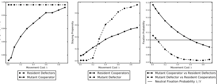
PSS0ρAS0 (26)
217
218
with boundary conditions
219
ρA∅ =0 and ρAN = 1. (27)
220 221
For typeB individuals we can use the fact thatρB
S = 1−ρAS.
222
We shall consider a population where a population is all of a single type, but
223
where a single population member is selected uniformly at random to be replaced
224
by one of the opposite type. We are thus interested in calculating the fixation
225
probability where state S consists of only one individual (all but one individual).
226
There are N initial states from which the fixation probability can be calculated,
227
and we take an arithmetic mean of these fixation probabilities, which we denote
228
as ρA (ρB). Alternatively, one could weight the fixation probability of a mutant
229
using the likelihood of that mutant appearing [4]. Sometimes this is an important
230
distinction, but in the examples considered in the current paper the differences are
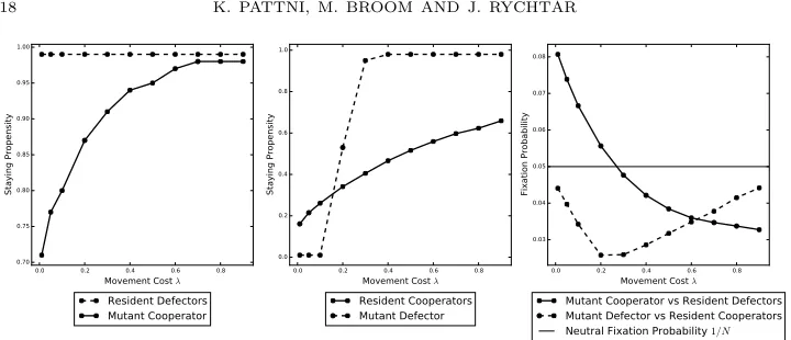
231
small, and so we have stuck with the traditional, simpler, version.
3. The Markov movement model. In the previous models [9] considered in
233
this framework, the movement of individuals is limited to their neighbourhood and
234
exogenously controlled by the home fidelity parameter that measures how likely
235
the individual is to remain in their home. A natural extension to this is to allow
236
individual distributions to vary with time. A logical first step is to consider a Markov
237
model, which is based on the assumption that history dependence is Markov, that is,
238
the current population distribution is only dependent upon the previous population
239
distribution. The concept of a Markov movement model within the framework was
240
introduced in [11], but was only discussed in general terms. In this paper we fully
241
develop it and apply it to example populations for the first time. The definitions
242
we have given before would then change as follows; for the PDPF we have
243
πt(m) =
X
m<t
pt(m|mt−1)P(m<t), (28) 244
245
for the mean change in fitness we have
246
¯
fn,t=
X
m
X
m<t
fn,t(m|m<t)pt(m|mt−1)P(m<t) (29) 247
248
and for the mean replacement weight change we have
249
¯
ui,j,t=
X
m
X
m<t
ui,j,t(m|m<t)pt(m|mt−1)P(m<t). (30) 250
251
3.1. Movement with dependence only upon individual history. In this
252
model it is assumed that an individual would move independently of the other
in-253
dividuals in the population but its current position is dependent upon its previous
254
position. The IDPF is then given as follows
255
πn,t(m) =
X
mn,<t
pn,t(m|mn,t−1)P(mn,<t). (31) 256
257
This expression can be rewritten using the M ×M probability matrix pn,t = 258
[pn,t(mn|mn,t−1)] formn, mn,t−1= 1, . . . , M as follows
259
πn,t=πn,0
t
Y
k=1
pn,k (32)
260
261
where πn,t = [πn,t(m)]m=1,...,M. Furthermore, if we assume that there is time 262
homogeneity, that ispn,t=pn for allt, then this simplifies to 263
πn,t =πn,0ptn. (33)
264 265
In this case, assuming thatpn is irreducible and aperiodic for alln, then ast→ ∞ 266
the IDPFπn,∞ is stationary for alln. Essentially, our model is then equivalent to
267
the fully independent movement model. We do not consider this case further here,
268
but rather refer the reader to [9] for a detailed discussion of this kind of model.
269
3.2. Individual movement with dependence on population history. In this
270
model individuals move to a new position independently of each other but dependent
271
upon the current distribution of the whole population. The IDPF is then as follows
272
πn,t(m) =
X
m<t
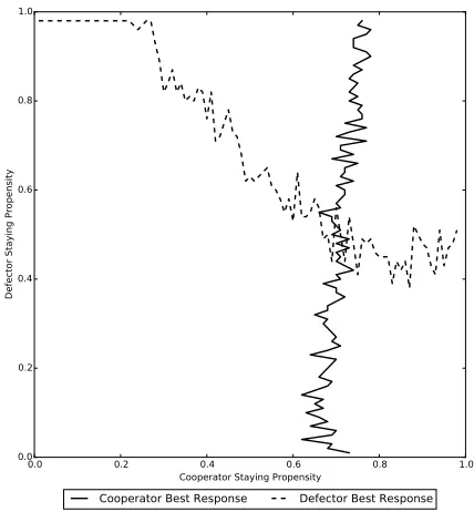
pn,t(m|mt−1)P(m<t). (34) 273
In this paper we construct a model of this type that is made up of the following
275
four components: population structure, movement strategy, game and evolutionary
276
dynamics.
277
3.2.1. The population structure. The population is assumed to be of sizeN where
278
each individuals has a home that they can return to. The structure is described by
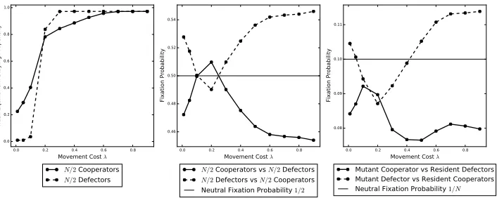
279
a graph such that each node represents a place. We consider the complete graph
280
structure where all places are connected to each other. We assume that every place
281
is home to precisely one individual.
282
3.2.2. Individual movement. We assume that the individual transition probabilities
283
are time homogeneous but dependent upon the previous group and previous position
284
of the individuals, that is
285
pn,t(m|mn,t−1,Gn(mt−1)) = (
hn(Gn(mt−1)) m=mn,t−1 1−hn(Gn(mt−1))
N−1 m6=mn,t−1
(35)
286
287
wherehn(Gn(mt−1)) denotes the staying probability of individualIn andN−1 is 288
the number of neighbouring places that an individual can move to in a complete
289
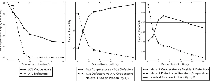
graph.
290
The staying probability hn(Gn(mt−1)) will depend upon thestaying propensity
291
αn of individual In and the attractiveness of remaining in group Gn(mt−1). The
292
staying propensity αn measures the likelihood that individualIn will stay where 293
it is, in particular, hn(Gn(mt−1)) = αn when In is alone (Gn(mt−1) ={n}). The
294
staying propensity is assumed to be one of the characteristics that makes up the type
295
of an individual. However, when present in a group (|Gn(mt−1)| >1), individual
296
In would take into account the benefit of remaining in that group. The benefit 297
βi of group memberIi to others depends upon itsinteractive strategy, the second 298
characteristic that makes up the type of an individual. We will assume that there
299
are two interactive strategies, cooperate (C) and defect (D). The benefit function,
300
βi is then defined as follows 301
βi=
(
βC ifIi cooperator, βD ifIi defector
(36)
302
303
whereβC andβD are thebenefits of being with a cooperator and defector, respec-304
tively. The benefit of groupGn(mt−1) to individualIn is then defined as follows 305
βGn(mt−1)\{n}=
X
i∈Gn(mt−1)\{n}
βi. (37)
306
307
Finally, combining the effects of the staying propensity and the group benefit, in
308
the rest of the paper the staying probability is expressed as the following sigmoid
309
function
310
hn(Gn(mt−1)) =
αn
αn+ (1−αn)SβGn(mt−1 )\{n}
(38)
311
312
where 0< S <1 is the sensitivity shown to group members. So, for example,S→0
313
implies thatInshows great sensitivity and would move away immediately if remain-314
ing in group Gn(mt−1) is unattractive, which is the case when βGn(mt−1)\{n} <0. 315
An alternative way of representing theS→0 limit involves the staying probability
being defined using the following step function
317
hn(Gn(mt−1)) =
0 |Gn(mt−1)|>1 andβGn(mt−1)\{n}<0, αn |Gn(mt−1)|= 1,
1 |Gn(mt−1)|>1 andβGn(mt−1)\{n}≥0.
(39)
318
319
For example, if we set αn = 0 ∀n, βC = 0 and βD < 0 then the attractiveness 320
of a group is completely determined by the presence or absence of defectors. An
321
individual would therefore leave with probability 1 if a defector is present in the
322
group. This was referred to as the ‘walk away’ strategy in [1].
323
In our model we select an exploration time T, which is the number of steps an
324
individual takes moving around the region before returning to its home place. Thus
325
the larger T, the more time cooperators have to find other cooperators, but also
326
the more time there is for them to be found by defectors.
327
3.2.3. Fitness. We assume that the change in fitness of an individual depends upon
328
direct group interactions and whether a movement has been made.
329
For these group interactions we will consider a public goods game in which the
330
payoffs are determined by the interactive strategies, cooperate and defect, that we
331
introduced earlier. Each individual receives a base reward of 1 regardless of their
332
strategy. A cooperator always pays a cost 0≤c <1 so that every individual that
333
it can directly interact with (excluding itself) receives an equal share of a reward
334
v >0. The cost cannot exceed 1 in order to prevent the fitness contribution from
335
going negative (this is done for convenience of calculation; it is important that total
336
fitness is not negative, and we could deal with large costs if necessary by truncating
337
the resulting total fitness at 0). A defector does not pay a cost but receives a share
338
of the reward from cooperators present in the group. Note that the base reward has
339
been normalised to 1 and the rewardv and costcare multiples of the base reward.
340
The direct group interaction payoff functions are then defined as follows
341
Rn,t(Gn(mt)) =
1 + |Gn(mt)|C−1
|Gn(mt)|−1 v−c In cooperator and|Gn(mt)|>1,
1−c In cooperator and|Gn(mt)|= 1,
1 + |Gn(mt)|C
|Gn(mt)|−1v In defector and|Gn(mt)|>1,
1 In defector and|Gn(mt)|= 1
(40)
342
343
where|G|C is the number of cooperators in groupG. Note the cooperators still pay 344
a cost when they are alone.
345
An individual will pay a cost of λ for every movement that it makes. The
346
movement cost is chosen so that it does not exceed the direct group interaction
347
payoff an individual receives (for the same reasons as for the cooperative cost c,
348
and large movement costs could be similarly accommodated if necessary), that is
349
0≤λ <min(Rn,t(Gn(mt))). The fitness contribution is then given by 350
fn,t(m,Gn(mt)|mt−1) = (
Rn,t(Gn(mt))−λ mt6=mt−1,
Rn,t(Gn(mt)) mt=mt−1.
(41)
351
352
It is clear that these fitness contributions vary with time, as the first move from
353
the home place follows the distribution for a lone individual, and then movement
354
depends upon the groups formed. For instance in a population entirely composed of
355
cooperators, individuals would almost cease to move when they had found another
356
cooperator, so the level of movement would decrease (and the fitness contributions
357
would increase) with time, until the exploration timeT is reached.
3.2.4. Evolutionary dynamics. We assume that the replacement weight
contribu-359
tion will only depend upon the direct group. As in [9], the replacement weight
360
contribution will depend upon the amount of time spent with each individual. In
361
particular, it is assumed that an individual spends an equal amount of time with
362
each individual in the group excluding itself. However, if the individual is alone,
363
then it effectively allocates all the time to itself. The replacement weight
contribu-364
tion function is then defined as follows
365
ui,j,t(Gi(mt)) =
1/|Gi(mt)\ {i}| i6=j andj ∈ Gi(mt),
0 i6=j andj /∈ Gi(mt),
1 i=j and|Gi(mt)|= 1,
0 i=j and|Gi(mt)|>1.
(42)
366
367
We note that combining equations (24) and (42), we have that wi,j =wj,i and 368
wi,i = 1−Pj6=iwi,j, which implies that our selected weights have the isothermal 369
property (see [31]).
370
3.2.5. Simulating the evolutionary Markov chain. The approach used in this paper
371
to calculate the fixation probability is a semi-analytic one where the fitnesses of
372
individuals are found by simulation, and these results are then used to evolve the
373
population using the evolutionary Markov chain, which results in a more accurate
374
solution than simulating the whole process (the movement process is too complex
375
to allow for a fully analytic solution).
376
Individuals start on their home place and then undergo an exploration phase of
377
T time steps as described in Section3.2.2. To calculate the fitness, the individuals
378
move T times such that their fitness contribution is calculated for each of these
379
movements; the total of these T fitness contributions gives their fitness for one
380
simulation. The position of the individuals is then reset, that is, they return to
381
their home place before the next simulation is run. Their average fitness for 10,000
382
simulations is used in the evolutionary Markov chain.
383
To calculate the replacement weights, individuals start on their home place and
384
move only one time to determine their replacement weight. This represents
indi-385
viduals returning to their home place to reproduce, with individuals being replaced
386
according to the corresponding local connections. This counts as one simulation
387
and, before the next simulation is run, we reset the position of the individuals so
388
they all start in their home place. The replacement weights are calculated exactly
389
because they comprise of only one movement. This involves calculating the
prob-390
ability that an individual is alone, which gives the self-replacement weight. The
391
other replacement weights are simply 1 minus the self-replacement weight divided
392
byN−1 because the probability of replacing the other individuals is the same for
393
a complete graph.
394
The fitnesses and the replacement weights are all that is required to construct
395
the transition probabilities of the evolutionary Markov chain. The transition
prob-396
abilities are substituted into the formula of [28] to give the fixation probability ofi 397
typeAmutants in a population ofN−itypeB residents as follows
398
ρAi =
1 +Pi−1
j=1 Qj
k=1
Pk− Pk+
1 +PN−1
j=1 Qj
k=1
Pk− Pk+
(43)
399
where Pk− (Pk+) is the backward (forward) transition probability for a state with
401
k type A individuals. Note that the weights wij and the fitnesses from Section 402
3.2.3depend upon the composition of the population, so at successive steps of the
403
evolutionary Markov chain the transition probabilities will in general be different.
404
We also note that this formula can easily be modified to find the fixation
proba-405
bility of typeB individuals. What exactly makes a type A orB individual would
406
depend upon its interactive strategy and staying propensity. For example, we could
407
have that A=C0.1 andB =D0.5, which means that typeAis a cooperator with
408
a staying propensity of 0.1 and type B is a defector with staying propensity 0.5,
409
or we could haveA=C0.1 andB=C0.2so both types have the same behavioural
410
strategy but different staying propensities. However, the important thing to note is
411
that, at any one time, there are only two unique typesA andB in the population.
412
The advantage of such an approach is that we can relatively quickly calculate the
413
fixation probability starting from any state. The saving comes from the fact that
414
we do not simulate the entire process, which would take much longer because the
415
number of steps to reach fixation could be high. However, this approach necessarily
416
requires that we have a population in which individuals can differ only in terms
417
of their type. To ensure that this is the case, we consider a complete structure
418
withN places such that each individual has their own home place.We note that the
419
advantage of efficient algorithmic processes over simulations was demonstrated in
420
[48], but also that it was shown in [27] that for frequency-dependent selection this
421
approach will not work for arbitrary spatial populations.
422
4. Results. In this section the effect of the model parameters on the fixation
prob-423
ability are investigated. In particular, we investigate how the model parameters
af-424
fectassortment, which is the mechanism that allows cooperation to evolve as shown
425
in [22]. There is positive assortment between cooperators if they are more likely
426
to interact with other cooperators than defectors. In our model, this occurs due
427
to an increase (decrease) in the time it takes for defectors (cooperators) to find
co-428
operators. According to [20] the time to find cooperators should depend upon the
429
density of the population and an individual’s movement speed. In their model,N 430
individuals pair up with one another to form a coalition such that the probability of
431
a pair forming is exponentially distributed with rateµ, which is a function ofN and
432
the population density. The time to find cooperators in their model is essentially
433
determined by the rateµ. We have one-to-one correspondence between individuals
434
and places and therefore the density remains constant; on the other hand, since we
435
consider a complete graph, the movement speed is high as individuals can directly
436
get from one place to another. Therefore, the time it takes to find cooperators is
437
mostly determined by the staying propensity of the individuals, however, this
rela-438
tionship is not so straightforward as it is not globally controlled and the individuals
439
may have different staying propensities (which are subject to the evolutionary
pro-440
cess). This means that some individuals may find cooperators faster than others.
441
The parameters used in the simulations are summarised in Table3.
442
Apart from an individual’s interactive strategy and staying propensity, all other
443
parameters are considered to be fixed. Each individual inherits these two
charac-444
teristics from its parent, and different interactive strategies or staying propensities
445
are introduced into the population through mutations. Staying propensities can
446
take any value 0.01mform= 1, . . . ,99; this means that no individual moves all the
447
time or never, and so makes some adjustment to their behaviour depending upon
Parameter Set 1 2 3 4 5 6
N 10 10 10 20 10 10
T 10 5 25 10 10 10
λ Variable Variable Variable Variable 0.20 0.20
c 0.04 0.04 0.04 0.04 0.04 0.09
[image:14.612.134.484.123.201.2]v 0.40 0.40 0.40 0.4 Variable Variable
Table 3. Parameters used for the simulations. The other
param-eters are fixed such that we have a complete structure with each individual having its own home, βC = 1, βD =−1,S = 0.03 and
the dynamics used are BDB.
the group they are in. In particular we have max(α) = 0.99; some movement is a
449
necessary requirement otherwise the replacement weights would be zero and there
450
would be no evolution within the population. In a real world setting, a minimum
451
movement requirement can be explained by, for example, foraging behaviour where
452
an individual searches its environment to find food and therefore needs to move in
453
order to survive.
454
The mutations of these characteristics are sufficiently infrequent that the
popu-455
lation is assumed to consist of a maximum of two types; resident and mutant, whose
456
competition will result in fixation of one of the types before a new mutant appears.
457
We consider two different scenarios to account for the different mutation rates of
458
each characteristic.
459
4.1. Scenario A: Interactive strategy mutations are rare. As previously
460
stated, it is assumed that fixation happens much faster than new mutations arise.
461
A mutation can result in a change of the interactive strategy and/ or the staying
462
propensity. In this scenario, the mutation rate of an individual’s interactive
strat-463
egy is much slower than the rate of mutations that involve their staying propensity.
464
Since it is much more likely that the staying propensity mutates than the
inter-465
active strategy does, once one of the interactive strategies (cooperate or defect) is
466
removed from the population, it will be a long time before a new mutant involving
467
this strategy appears. During this time, there will be a sequence of contests among
468
individuals with the same interactive strategy but different staying propensities and
469
the population will eventually evolve to the point where all individuals have the
470
same interactive strategy and are using a (strict) Nash equilibrium staying
propen-471
sity (a strict Nash equilibrium propensity is one where the fixation probability is
472
maximised and changing the staying propensity is disadvantageous). Eventually, a
473
mutant with a different interactive strategy and staying propensity will appear, and
474
the quantity of interest at this point is the fixation probability of this mutant type.
475
We assume that the staying propensity of the mutant can be different from the
476
Nash equilibrium staying propensity of the resident population it is invading. The
477
resident population will therefore be stable if it can resist invasion from a mutant
478
using any staying propensity. Rather than considering any arbitrary mutant, the
479
focus will be on the mutant most likely to invade, i.e. one maximising its fixation
480
probability.
Cooperator residents are of the typeCγR where their Nash equilibrium staying
482
propensityγR is the staying propensity wherea=bin the set 483
n
(a, b) :ρCa,Cb
1 = max
ρCc,Cb
1 :c∈(0,1)
andb∈(0,1)o. 484
485
In this set we identify all the points (a, b) where a is the best response staying
486
propensity of 1 individual of typeCa when playing againstN−1 individual of type 487
Cb, who are using some arbitrary staying propensity b. Therefore, at the point 488
wherea=b, Ca is a best response to itself, i.e. a Nash equilibrium. 489
A defector mutant is of the typeDδM where the staying propensity δM satisfies
490
ρ1DδM,CγR = maxρ1Dc,CγR :c∈(0,1). 491
492
Defector residents are of the typeD0.99(i.e. in the equivalent terminology to the
493
aboveδR= 0.99) where their Nash equilibrium staying propensity is max(α) = 0.99 494
whenever the movement cost is greater than 0 because the only way for them to
495
maximize their fixation probability is by moving as little as possible.
496
A cooperator mutant is of the typeCγMwhere the staying propensityγM satisfies
497
ρC1γM,D0.99 = maxρCc,D0.99
1 :c∈(0,1)
. 498
499
The Nash equilibrium staying propensity of the resident cooperators γR is cal-500
culated as follows. We considerN −1 residents of the type Cb and calculate the 501
fixation probability of 1 individual of the typeCa for all values of ain the range 502
[max(0.01, b−0.09),min(b+ 0.09,0.99)], and the a that gives the highest fixation
503
probability is picked. Note that using a wider range of values foragives the same
504
result so this range is used for efficiency. TheN−1 residents then use the staying
505
propensityathat was picked and this process is repeated several times. After around
506
20 repetitions, the staying propensity that gives the maximum fixation probability
507
remains the same, that is, we can see that is a (strict) Nash equilibrium because
508
it is a best response to itself and any other strategy will be disadvantageous. We
509
therefore setγR to the value ofawe get after 20 repetitions. 510
We hypothesize that there is only one solution to the Nash equilibrium staying
511
propensity. As seen in Figure 1, the best response staying propensity of one type
512
Ca against N −1 type Cb is relatively flat (the jagged line of the figure being 513
an approximation to a smooth “real” value, caused by the stochasticity of the
514
simulations). Intuitively the real solution should be smooth; a small change in the
515
movement cost would have a small change on the payoff to a focal individual. It is
516
possible that at some point this would lead to a sudden jump of the best response
517
strategy as the payoffs from two different values pass. We would expect to see either
518
a single smooth continuous function for the best response, or a piecewise continuous
519
collection of distinct parts, and it is the former that we have here. This flatness
520
means that the best response staying propensity is predominantly determined by
521
the movement cost λ regardless of what the other players are doing. Therefore,
522
there is only one intersection point with the linea=bas shown in Figure1, which
523
gives the Nash equilibrium staying propensityγR of resident cooperators. A non-524
unique solution would occur if there were multiple crossings (or indeed no crossings,
525
which would need a discontinuity in Figure1, as described above). We should note
526
that we have no proof of the uniqueness of the Nash equilibrium staying propensity,
527
although in all cases considered, the solution to the process described in the previous
528
paragraph is independent of the starting position.
0.0 0.2 0.4 0.6 0.8 1.0 Staying Propensity j of N−1 type Cj
0.0 0.2 0.4 0.6 0.8 1.0
St
ay
ing
Pr
op
en
sit
y o
f
1
ty
pe
Ci
[image:16.612.200.413.120.351.2]Best response staying propensity of 1 type Ci i=j
Figure 1. This plot shows the best response staying
propen-sities for 1 type Ci individual playing against N −1 type Cj
individuals. Parameter set 1 is used with λ = 0.2 and i, j ∈ {0.01,0.02, . . . ,0.99}. The intersection point of the plots gives the unique strategy which is a best response to itself, i.e. the unique cooperator resident Nash equilibrium staying propensityγR, which
is somewhere between 0.3 and 0.4. This value is similar to the one obtained using the iterative method (see Figure2). The val-ues from the current figure are approximate only because of the jagged nature of the lines; these occur because of the very large number of simulations that would be necessary to obtain a smooth version (the figure uses 10000 simulations for each combination). The figure is used to illustrate the uniqueness of the solution only.
4.1.1. The effect of the movement cost. In Figure 2 the effect of the movement
530
cost is shown. In particular, it increases the time it takes to find cooperators by
531
increasing the staying propensity, that is,γR, γM, δM are positively correlated with 532
movement cost; the (partial) exception is resident defectors, which we know have a
533
staying propensity of max(α) = 0.99 regardless of the movement cost.
534
For very low movement cost, both mutant types have a significantly lower staying
535
propensity than the resident population that they are invading. They can therefore
536
invade the resident population because they take less time to find cooperators.
537
For higher, but still low, movement costs, whilst mutant cooperators can still
538
invade, mutant defectors cannot. Here the resident cooperators are better at
pre-539
venting invasion even whenδM < γR for some values of the movement cost. This 540
is because the movement cost impacts the invading mutant defector more adversely
541
than the resident cooperators, who on average leave and regroup less often than a
542
defector who will be repeatedly deserted by its cooperator groupmates.
For intermediate movement costs, neither mutant type can invade. At this point,
544
sinceδM > γR, a mutant defector is slower at finding cooperators than the resident 545
cooperators and therefore cannot take advantage of them. For a mutant cooperator,
546
γM becomes much larger thereby diminishing their advantage over the resident 547
defectors, in particular, not only are they paying a higher movement cost but it
548
takes longer to find the other cooperators, which in turn reduces the amount of
549
time that they can spend with them.
550
For high movement costs, defecting mutants can invade, but cooperator mutants
551
cannot. At this point all types have a large staying propensity and therefore do
552
not interact much with one another. However, a mutant defector is helped by the
553
fact that the resident cooperators always pay a cooperating cost that they now find
554
difficult to recoup because they are moving very little and also paying a very large
555
movement cost whenever they do so.
556
0.0 0.2 0.4 0.6 0.8
Movement Cost λ 0.75
0.80 0.85 0.90 0.95 1.00
Staying Propensity
Resident Defectors Mutant Cooperator
0.0 0.2 0.4 0.6 0.8
Movement Cost λ 0.0
0.2 0.4 0.6 0.8 1.0
Staying Propensity
Resident Cooperators Mutant Defector
0.0 0.2 0.4 0.6 0.8
Movement Cost λ 0.08
0.09 0.10 0.11 0.12
Fixation Probability
Mutant Cooperator vs Resident Defectors Mutant Defector vs Resident Cooperators
[image:17.612.126.485.292.426.2]Neutral Fixation Probability 1/N
Figure 2. These plots show the effect of movement cost on the
evolution of cooperation using parameter set 1. The left (centre) plot shows the staying propensities δR = 0.99 (γR) for resident
defectors (cooperators) andγM (δM) for a mutant cooperator
(de-fector) used to invade the resident population. In the right plot, we have the fixation probability of a mutant cooperatorCγM (defector
DδM) againstN−1 resident defectorsD0.99 (cooperatorsCγR).
4.1.2. The effect of the exploration time. The exploration timeTplays an important
557
role in the evolution of cooperation. Changing the exploration time has a minimal
558
effect on the time it takes to find cooperators because it will not alter the speed of
559
movement of the individuals. This is because we are using a complete graph and
560
individuals can directly get from one place to any other. However, increasing the
561
exploration time has a positive effect on the coalition time, that is, the amount
562
of time that cooperators spend cooperating with one another. [20] showed that
563
increasing the coalition time helps with the evolution of cooperation. In our model,
564
one explanation for this is that the fitness of the individuals, which is the average
565
reward over the exploration time, will naturally have a higher value the larger the
566
coalition time.
567
In Figure 3 reducing the exploration time T from 10 to 5 steps decreases the
568
coalition time which adversely affects the cooperators. One of the key differences
569
is that the resident cooperators now find it much more difficult to prevent invasion
from a mutant defector. The shape of the plot for a mutant cooperator is largely
571
the same but with a consistently lower fixation probability. In Figure4 increasing
572
the exploration timeT from 10 to 25 steps benefits the cooperators. Not only does
573
it help the resident cooperators prevent invasion from a mutant defector but it also
574
increases the success of an invading mutant cooperator. This again has to do with
575
the increased coalition time that allows the cooperators to increase their fitness.
576
0.0 0.2 0.4 0.6 0.8
Movement Cost λ 0.70
0.75 0.80 0.85 0.90 0.95 1.00
Staying Propensity
Resident Defectors Mutant Cooperator
0.0 0.2 0.4 0.6 0.8
Movement Cost λ 0.0
0.2 0.4 0.6 0.8 1.0
Staying Propensity
Resident Cooperators Mutant Defector
0.0 0.2 0.4 0.6 0.8
Movement Cost λ 0.08
0.09 0.10 0.11 0.12
Fixation Probability
Mutant Cooperator vs Resident Defectors Mutant Defector vs Resident Cooperators
[image:18.612.130.484.209.344.2]Neutral Fixation Probability 1/N
Figure 3. Plots created using parameter set 2. The exploration timeT has been decreased from 10 to 5.
0.0 0.2 0.4 0.6 0.8
Movement Cost λ 0.80
0.85 0.90 0.95 1.00
Staying Propensity
Resident Defectors Mutant Cooperator
0.0 0.2 0.4 0.6 0.8
Movement Cost λ 0.0
0.2 0.4 0.6 0.8
Staying Propensity
Resident Cooperators Mutant Defector
0.0 0.2 0.4 0.6 0.8
Movement Cost λ 0.07
0.08 0.09 0.10 0.11 0.12 0.13 0.14 0.15
Fixation Probability
Mutant Cooperator vs Resident Defectors Mutant Defector vs Resident Cooperators
Neutral Fixation Probability 1/N
Figure 4. Plots created using parameter set 3. The exploration
timeT has been increased from 10 to 25.
4.1.3. The effect of population size. Fixation probability is reduced in general when
577
the size of the population increases, as we see when comparing Figures 2 and 5,
578
with population sizes of 10 and 20 respectively. The key value to compare fixation
579
probabilities against is the neutral fixation probability of 1/N, the horizontal line
580
in each of these figures, however. We see that the fixation probability is slightly
581
higher for cooperators when compared to this line for the larger population of Figure
582
5 (although it is also more sensitive to the movement cost) than for the smaller
583
population. The key difference is that a mutant defector has fixation probability
584
consistently under the neutral line in Figure5 and so cannot invade even for very
[image:18.612.132.485.409.546.2]0.0 0.2 0.4 0.6 0.8 Movement Cost λ 0.70
0.75 0.80 0.85 0.90 0.95 1.00
Staying Propensity
Resident Defectors Mutant Cooperator
0.0 0.2 0.4 0.6 0.8
Movement Cost λ 0.0
0.2 0.4 0.6 0.8 1.0
Staying Propensity
Resident Cooperators Mutant Defector
0.0 0.2 0.4 0.6 0.8
Movement Cost λ 0.03
0.04 0.05 0.06 0.07 0.08
Fixation Probability
Mutant Cooperator vs Resident Defectors Mutant Defector vs Resident Cooperators
[image:19.612.127.487.103.258.2]Neutral Fixation Probability 1/N
Figure 5. Plots created using parameter set 4. The population
size has been increased from 10 to 20.
low movement cost in the larger population. Thus larger populations help a little
586
in establishing cooperation, but help a lot in making it stable against defection.
587
Increasing the population size has a positive impact on the evolution of
cooper-588
ation because it increases the time it takes to find cooperators. Note that we are
589
assuming that there is a one-to-one correspondence between individuals and places
590
and therefore increasing the number of individuals also increases the number of
591
places. Even though the density remains the same, there would be more places for
592
the individuals to search in order to find cooperators thereby increasing the overall
593
time it takes to find cooperators. In particular, an individual that is currently not
594
in a cooperating group will have to searchN−1 places to find one, therefore, the
595
probability of a defector finding a cooperating group decreases as N gets larger.
596
This means that cooperators would resist invasion by defectors better, as we have
597
noted above.
598
4.1.4. The effect of reward and cost. The reward to cost ratio v/c is important
599
because, even if other external factors favour cooperation, cooperation will not
600
evolve if the reward to cost ratio is too low. This is seen in Figure 6 where the
601
cost is set to 0.04 with the reward written as a multiple of the cost. When v/c 602
is low, a mutant cooperator cannot invade but a mutant defector can. This is
603
simply because the value of v/cis too low to promote cooperation. Increasingv/c 604
makes cooperation more viable and, in particular, it allows a mutant cooperator to
605
reduce the time it takes to find cooperators by reducing its staying propensity. It
606
becomes more difficult for a mutant defector to invade because, on average, resident
607
cooperators move less than the mutant defector as they are more in number and the
608
largerv/chelps them quickly recoup any movement cost they incur whilst evading
609
the mutant defector. This is the case even whenδ < γR, that is, a mutant defector 610
takes less time to find cooperators. For comparison with a different value ofv/c, in
611
Figure 7the cost is set to 0.09. However, there is no fundamental change in what
612
happens and we have a very similar figure to that forc= 0.04.
613
4.2. Scenario B: Interactive strategy mutation is not rare. In this scenario,
614
the mutation rate of an individual’s interactive strategy is not much slower than that
615
of their staying propensity. Since the staying propensity would take a number of
616
mutations to reach the right level for any scenario, any successful strategy will have
0 10 20 30 40 50 Reward to cost ratio v/c 0.84
0.86 0.88 0.90 0.92 0.94 0.96 0.98
Staying Propensity
Resident Defectors Mutant Cooperator
0 10 20 30 40 50
Reward to cost ratio v/c 0.0
0.2 0.4 0.6 0.8 1.0
Staying Propensity
Resident Cooperators Mutant Defector
0 10 20 30 40 50
Reward to cost ratio v/c 0.06
0.08 0.10 0.12 0.14 0.16 0.18
Fixation Probability
Mutant Cooperator vs Resident Defectors Mutant Defector vs Resident Cooperators
[image:20.612.131.487.103.260.2]Neutral Fixation Probability 1/N
Figure 6. Plots have been created using parameter set 5. The
plots here are against the reward to cost ratiov/c such that c = 0.04.
0 10 20 30 40 50
Reward to cost ratio v/c 0.84
0.86 0.88 0.90 0.92 0.94 0.96 0.98
Staying Propensity
Resident Defectors Mutant Cooperator
0 10 20 30 40 50
Reward to cost ratio v/c 0.0
0.2 0.4 0.6 0.8 1.0
Staying Propensity
Resident Cooperators Mutant Defector
0 10 20 30 40 50
Reward to cost ratio v/c 0.10
0.15 0.20
Fixation Probability
Mutant Cooperator vs Resident Defectors Mutant Defector vs Resident Cooperators
[image:20.612.129.488.315.455.2]Neutral Fixation Probability 1/N
Figure 7. Plots have been created using parameter set 6. The
plots here are against the reward to cost ratiov/c such that c = 0.09.
to repeatedly face individuals of both types. The (strict) Nash equilibrium staying
618
propensity will then be determined in a mixed population, i.e. there are individuals
619
of both types. For simplicity we choose only one mixed state to determine the Nash
620
equilibrium staying propensity which is the one where there areN/2 individuals of
621
each type. The Nash equilibrium staying propensity for each type is therefore the
622
one in which the fixation probability from the mixed state of each type is maximised.
623
Resident and mutant defectors are of the same type Dδ. Similarly, resident 624
and mutant cooperators are of the same type Cγ. The Nash equilibrium staying 625
propensitiesδandγ are determined by the intersection of the following two sets
626
n
(a, b) :ρCa,Db
N/2 = max
ρCc,Db
N/2 :c∈(0,1)
andb∈(0,1)o, 627
n
(a, b) :ρDb,Ca
N/2 = max
ρDc,Ca
N/2 :c∈(0,1)
anda∈(0,1)o. 628
629
In the first set we are finding the Nash equilibrium staying propensityaofN/2 type
630
Ca playing against N/2 type Db, whereb is some arbitrary staying propensity. In 631
the second set we are finding the Nash equilibrium staying propensitybofN/2 type
Db playing againstN/2 typeCa, whereais some arbitrary staying propensity. The 633
point at which these two sets intersect is (γ, δ), that is, both types will be using
634
their Nash equilibrium staying propensities.
635
To calculate γ and δ we use a similar iterative procedure from scenario A. To
636
initialise the iterative procedure we arbitrarily choose some staying propensitiesa0
637
and b0, and the iterative step is as follows. We calculate the fixation probability
638
of N/2 type Ca individuals against N/2 type Db0 for all values of ain the range 639
[max(0.01, a0−0.09),min(a0+ 0.09,0.99)]. The staying propensityathat gives the
640
maximum fixation probability is picked, which is labelleda1. We then calculate the
641
fixation probability ofN/2 typeDb individuals againstN/2 typeCa1 for all values 642
ofbin the range [max(0.01, b0−0.09),min(b0+ 0.09,0.99)]. The staying propensity
643
bthat gives the maximum fixation probability is picked, which is labelledb1. Note
644
that using a wider ranges for a and b gives the same result so these ranges were
645
used for efficiency. After around 20 repetitions of the iterative step, the staying
646
propensitiesaandb that give the maximum fixation probability remain the same,
647
which means that we are at a (strict) Nash equilibrium because any other values
648
would be disadvantageous. We therefore setγ=a20andδ=b20.
649
We hypothesize thatγandδare unique. For cooperators, their Nash equilibrium
650
staying propensity is relatively stable because it is predominantly determined by the
651
movement cost regardless of what the defectors are doing. As seen in Figure8, the
652
plot for this is a roughly vertical line. For defectors, their Nash equilibrium staying
653
propensity is negatively correlated with the staying propensity of the cooperators
654
given that the movement cost is not too large, otherwise it would be max(α). In
655
Figure8, the plot for this slopes downwards as the staying propensity of the
coop-656
erators increases. There is therefore only one intersection point of the two curves
657
that givesγ andδ.
658
4.2.1. The effect of movement cost. As in scenario A, the movement cost increases
659
the staying propensity of the individuals and, therefore, increases the time it takes
660
to find cooperators. As seen in Figure9, what happens in this case is quite different
661
to the situation in scenario A. Here, the mutant cooperator does not benefit from
662
the fact that the resident defectors have a very high staying propensity as in scenario
663
A. In this case,δchanges with the movement cost in a similar way thatγ changes.
664
Therefore, the key difference here is that a mutant cooperator cannot invade for
665
very low movement cost because the resident defectors have a very low staying
666
propensity, which means that they take much less time to find cooperators.
667
4.2.2. The effect of exploration time. As in scenario A, the cooperators do worse
668
when the exploration time is lower; this is shown in Figure10whereT is decreased
669
from 10 to 5, and in Figure11whereT is increased from 10 to 25. The explanation
670
is as in scenario A where the coalition time is lower when the exploration time is
671
lower and the coalition time increases, since, as we already know, increasing the
672
coalition time helps the cooperators do better.
673
4.2.3. The effect of population size. Similarly to scenario A, increasing the
popu-674
lation size helps cooperators as shown in Figure12, where N is increased from 10
675
to 20. As before, increasing the population size increases the time it takes to find
676
cooperators because there is a one-to-one correspondence between individuals and
677
places. Increasing the population size therefore increases the number of places that
678
need to be searched to find cooperators. Furthermore, as in scenario A, a mutant
679
defector can no longer invade resident cooperators for very small movement cost.
0.0 0.2 0.4 0.6 0.8 1.0 Cooperator Staying Propensity
0.0 0.2 0.4 0.6 0.8 1.0
Defector Staying Propensity
[image:22.612.199.413.120.351.2]Cooperator Best Response Defector Best Response
Figure 8. This plot shows the best response cooperator staying propensity (solid line, value shown on the x-axis) versus the range of defector staying propensities on the y-axis, and the best response defector staying propensity (dashed line, value shown on the y-axis) versus the range of cooperator staying propensities (on the x-axis) for N/2 cooperators and N/2 defectors. Parameter set 1 is used with λ = 0.2 and the staying propensities are chosen from the set {0.01,0.02, . . . ,0.99}. The best response staying propensities cross at one point only, which is thus the unique Nash equilibrium, where γ ≈ 0.7 and δ ≈ 0.5. These values are similar to those obtained using the iterative method described earlier (see Figure
9). As before, the values from the current figure are approximate only because of the jagged nature of the lines; the figure is used to illustrate the uniqueness of the solution only.
4.2.4. The effect of reward and cost. For a mutant defector, the effect of the reward
681
to cost ratio v/cis the same as in scenario A. However, a mutant cooperator does
682
not do better with increasing v/c. In this scenario, the fixation probability of a
683
mutant cooperator peaks, then starts dropping, asv/cis increased. This is because
684
the resident defectors have a very low staying propensity, and are therefore faster at
685
finding cooperators, making it difficult for a mutant cooperator to invade because it
686
cannot avoid the defectors. This is shown in Figure13wherec = 0.04. Increasing
687
the costcthough, makes it even more difficult for the cooperators regardless ofv/c.
688
In Figure 14, a mutant cooperator cannot invade for any v/c. This is because a
689
largercreduces the cooperators’ background fitness by a larger amount, increasing
690
the handicap that the cooperators already have.
691
4.3. The effect of other parameters. The effects of other parameters are not
692
shown using plots but will be explained in this section.