Gregory Bentsen,1 Tomohiro Hashizume,2 Anton S. Buyskikh,2 Emily J. Davis,1 Andrew J. Daley,2 Steven S. Gubser,3 and Monika Schleier-Smith1
1
Department of Physics, Stanford University, Stanford, CA 94305, USA 2Department of Physics and SUPA, University of Strathclyde, Glasgow G4 0NG, UK
3
Department of Physics, Princeton University, Princeton, NJ 08544, USA
(Dated: October 26, 2019)
We propose an experimentally realizable quantum spin model that exhibits fast scrambling, based on non-local interactions which couple sites whose separation is a power of 2. By controlling the relative strengths of deterministic, non-random couplings, we can continuously tune from the linear geometry of a nearest-neighbor spin chain to an ultrametric geometry in which the effective dis-tance between spins is governed by their positions on a tree graph. The transition in geometry can be observed in quench dynamics, and is furthermore manifest in calculations of the entanglement entropy. Between the linear and treelike regimes, we find a peak in entanglement and exponen-tially fast spreading of quantum information across the system. Our proposed implementation, harnessing photon-mediated interactions among cold atoms in an optical cavity, offers a test case for experimentally observing the emergent geometry of a quantum many-body system.
The fast scrambling conjecture—inspired by studies of the black-hole information problem—predicts a lower bound on the time for information to spread from one to all degrees of freedom of an N-body quantum sys-tem, scaling as t∗ ∝ log(N) [1, 2]. Fast scrambling is conceptually important as a putative signature of the quantum physics of black holes [3]. It is also of prac-tical importance because a fast scrambler is an efficient quantum encoder, capable of quickly entangling quantum information across many physical qubits [4]. While infor-mation scrambling has been probed in several pioneering experiments [5–8], observingfast scrambling remains an outstanding challenge.
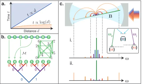
In typical quantum systems found in nature, fast scrambling is precluded by the locality of interactions. In the presence of only short-range interactions, infor-mation propagation is bounded by a linear “light cone” [9–12] (Fig. 1a), such that the scrambling time is at least
t∗ ∝ N. Even with long-range power-law interactions [13–15], the time for quantum correlations to propagate scales polynomially with distance [14, 15] and not loga-rithmically. Potential work-arounds include engineering interactions among spatially overlapped modes [16–18] or using light to mediate effectively non-local interactions [19, 20]. Proposals to date have focused on emulating solvable models for fast scrambling featuring random all-to-all couplings [16–18, 20].
In this Letter, we propose an experimentally realizable quantum spin model featuring a sparse, deterministic graph of non-local interactions that enables fast scram-bling. A modest generalization of the simplest model provides a smooth interpolation between two radically different notions of geometry: linear or treelike, as shown in Fig. 1b. Our simplest model is, in a certain sense, exactly between these two limits. Instead of exhibiting extended spatial geometry, it is fully characterized by a coupling graph whose diameter grows logarithmically
ω
ω
Distance
Time
ω0 ωl
( ) ( )
( )
a. c.
b. 0 1 2 3 4 5 6 7
0 0
0 1
1 0 1
1
0 4 2 6 1 5 3 7
0 1 0 1 0 1
i.
[image:1.612.318.563.278.423.2]ii.
FIG. 1. Nonlocal spin models with cold atoms. (a) Lin-ear light cone vs. fast scrambling. (b) Spins (green) coupled locally along a chain of lengthN = 8 or non-locally accord-ing to a tree of depthn = log2(N). Green cube shows full pattern of couplings specified in Eq. (2). (c) Scheme for con-trolling the graph of interactions mediated by a cavity via the spectrum of a drive field and the gradient of a magnetic fieldB. Depending whether short-range (blue) or long-range (orange) couplings dominate, the graph resembles either the linear chain (i) or the tree (ii).
works have suggested that diffusion on the Bruhat-Tits tree can be used to understand aspects of fast scrambling near black hole horizons [23, 24].
The models we consider here are inspired by an ele-gant proposal [25] for engineering translation-invariant long-range interactions by encoding spins in cold atoms coupled to light in a waveguide or cavity [26–37]. This scheme can generate Hamiltonians of the form
H = 1
2S X
i,j
J(i−j)Si+Sj−, (1)
wherei, j= 1, . . . , N, andSi is a spin-S operator repre-senting either an individual atom or the collective spin of a small atomic ensemble at site i. We consider a sparse graph of couplings between sites separated by powers of two,
J(i−j) =
(
Js2`s when|i−j|= 2`, `= 0,1,2,3. . .
0 otherwise,
(2) where by tuning the exponent s from −∞ to +∞ we interpolate between the linear and treelike limits. The simplest choice s = 0, where all non-zero couplings are equal, permits a perturbation to spread exponentially be-cause the number of pairwise interactions required to get from site ito site j is bounded above by the number of binary digits iniandj that differ.
The couplings in Eq. (2) can be generated by a pair of Raman processes wherein one atom flips its spin by virtually scattering a photon from a control field into a cavity, and a second atom rescatters this photon such that its spin flops [31]. In a magnetic field gradient [25], the energy cost of a flip-flop is proportional to the dis-tance d = i−j between spins. Thus, inducing reso-nant flip-flops at distance |d| = 2` requires modulating the control field at a frequencyω` ∝d. More generally, weakly modulating the control field at multiple frequen-cies ω` for ` = 0,1,2,3, . . . produces a set of sidebands whose amplitudes dictate the hopping amplitudes J(d) (Fig. 1).
Below, we take N a power of 2 and assume periodic boundary conditions unless otherwise stated, letting |x| denote the minimum value ofp(x+qN)2 over all inte-gersq. We normalize the couplings in Eq. (2) such that the largest is always a constant J0, letting Js = J0 for
s≤0 andJs=J0(N/2)−s fors >0.
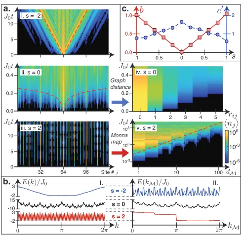
The key features of our spin model are evident already in the spreading of a single initially localized spin excita-tion (Fig. 2a), which is governed by the magnon disper-sion relation (Fig. 2b)
E(k) = 2Js
log2(N/2)
X
`=0
2`scos(2`k), (3)
wherek∈[0,2π) is the wavenumber. Intriguingly, asN
increases, the dispersion relation shows fractal behavior -2
-10
-2 15
3
3 i. ii.
b.
s = -2 s = 0 s = 2
Site # 64 96 32
a.
Monna map
10-3
100
103
1 10 100
c.
Graph distance 0.2
0.4
0.0
5 10
0
0.2 0.4
0.0
0 1 2 3 4 5
10-6
100
10-3 i. s = -2
ii. s = 0
iii. s = 2 v. s = 2
0 0.5 1
-0.5 -1 1.0
0.5
0.0
iv. s = 0
5 10
0
2
[image:2.612.317.561.49.288.2]1
FIG. 2.Dynamics in the single-magnon sector. (a) Oc-cupation hnj(t)i forN = 128 sites initialized with a single excitation on site N/2 with (i)s = −2, (ii) s = 0, or (iii) s= 2; slowest-growing occupations are bounded from above by dashed red lines. (iv) Occupationhnj(t)i at s = 0 for N = 1024, vs. graph distance rij from initial site i. (v) Reemergence of light cone ats= 2 after rearrangingN = 128 sites according to Monna mapM. (b) Magnon dispersion re-lation forN = 128 sites arranged according to either (i) phys-ical location or (ii) Monna-mapped order fors=−2 (blue), s = 0 (black), and s = 2 (red). (c) Breakdown of polyno-mial light cone: polynopolyno-mial exponentb(red) and logarithmic exponentc0 (blue) versuss.
converging to a Weierstrass function for 0< s < 1 [38]. For arbitrarys, Eq. (3) allows us to analytically compute the single-magnon dynamics as shown in Fig. 2a, where we introduce a single excitation on sitei=N/2 and plot the mean occupationhnj(t)ias a function of site number
j and timet.
because many small steps can be combined into a large jump.
We can understand the 2-adic norm as a tree-like mea-sure of distance because|i−j|2= 2dtree(i,j)/2/N, where dtree(i, j) is the number of edges between sites i and j along the regular tree in Fig. 1b [39]. The leaves are numbered in order of increasing M(i), where the dis-crete Monna map M reverses the bit order in the site number. For example, for N = 8 sites, M(1) = 4 be-cause in binary, M(0012) = 1002. Noting that N k/2π is an integer, we may likewise define a Monna-mapped wavenumberkM by
NkM
2π =M
N k
2π
. (4)
For large positive s, we rearrange the spins according to the Monna map and find that a light cone reappears (Fig. 2a(v)) and the dispersion relation is smoothed out (Fig. 2b), corroborating the transformation to the tree-like geometry defined by the 2-adic norm.
The radical difference between Archimedean and ul-trametric geometry raises the question of what happens near s = 0, where short- and long-range couplings are equally strong. Here, it is useful to think of the sites as arranged on a hypercube [40], where each site number in binary specifies a corner. The coupling graph consists of the edges of the hypercube plus some diagonals, as shown in Fig. 1b forN = 8 sites. For anyN, thegraph distance
rijcounts the minimum number of edges required to con-nect sitesiandj, and is at mostd1
2log2(N)e, wheredxe denotes the smallest integer greater than or equal tox.
We expect the logarithmic diameter of the interac-tion graph at s = 0 to enable a localized perturbation to spread over the entire system in a logarithmic time
t∝log(N). As a first test, in Fig. 2a we examine single-magnon transport as a function of both physical distance
d = |i−j| and graph distance rij. We observe spin transport on a timescale that is roughly linear in graph distance (Fig. 2a(iv)), and thus at most logarithmic in physical distancedand system sizeN.
To permit this logarithmic timescale, the polynomial light cone in Fig. 2a(i) must break down assapproaches 0. To examine this breakdown, we evaluate the timet for the magnon occupation at a distancedfrom the initial site to reach a threshold valuehni+di== 1/N2. For arbitrary s, we may always bound t from below by a polynomial of the form ad(M)
b
≤ t that depends on physical distanced for s ≤0 or Monna distance dM ≡ M(d) for s > 0, with non-negative constants a, b. We determine the dependence of the exponentbonsfrom a fit to the points of fastest growth [41] in Fig. 2a, finding a direct proportionalityb∝ |s|(red points in Fig. 2c). The vanishing exponentbat s= 0 signifies the breakdown of the polynomial light cone.
Furthermore, we verify that even the slowest-growing occupations take only a logarithmic time to reach the
-2 0
A
rchimedean
2-adic
2
-2 0 2
0 .5 1
0 1 2 3 4 5 6 7 0 4 2 6 1 5 3 7
Archimedean 2-adic
1
0 2
a.2 b.
1
0
8 16
Exponent
[image:3.612.320.562.52.159.2]Entanglement Entropy
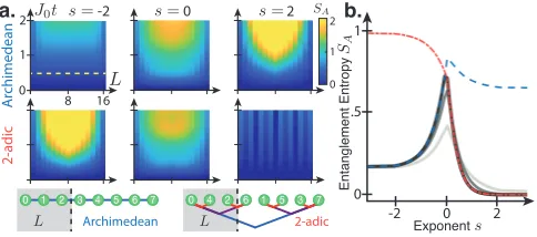
FIG. 3.Growth of entanglement after a quench,for an initial product state ofN = 16 sites with S = 1/2 oriented alongxˆ. (a) Entanglement entropySA vs. partition size L and time t, for Archimedean (top) or 2-adic (bottom) par-titions. (b) Minimum entanglement vs. s over all possible partitions of sizeL = 1,2,4,8 (light to dark solid curves), compared with entanglement for Archimedean (blue dashed) and 2-adic (red dot-dashed) partitions.
threshold. For arbitrarys, the timetis bounded above by t ≤ a0
d(M)
b0
logd(M)
c0
, with non-negative con-stants a0, b0, c0 (dashed red lines in Fig. 2a) [41]. Here, as s → 0 the polynomial exponent b0 again disappears, but the logarithmic exponentc0 remains (blue points in Fig. 2c). For both the fastest- and slowest-growing oc-cupations we observe an approximate symmetry about
s= 0 that suggests a duality between the Archimedean and non-Archimedean regimes [44].
While the spin dynamics provides strong evidence for the underlying geometry of the model as a function ofs, the structure of entanglement provides an even sharper proxy for locality. We analyze the growth of entangle-ment for a system initialized in a product state of spins polarized along xˆ. Figure 3a shows the entanglement entropy SA of a subsystem A as a function of its size and time, with the spins partitioned either according to their physical position (top) or to their Monna-mapped ordering (bottom). In either of the two limits where|s| is large, there is a natural way of partitioning the sys-tem such that entanglement remains low, as summarized in Fig. 3b: for s < 0, the cut must be between nearest neighbors in the linear chain (blue curve), whereas for
s >0 the cut must be between branches of the tree (red curve).
Near s= 0, however, entanglement is high no matter how we cut the system. We verify this by plotting the minimum entanglement entropy over all possible bipar-titions, without regard to locality. The resulting gray curves in Fig. 3b, for different partition sizes L, show a sharp peak in entanglement at s = 0. Thus, at the crossover between the Archimedean and 2-adic geome-tries, there is no good notion of locality, and all spins are strongly coupled to one another.
Our non-local spin models generically exhibit quantum chaos. One indicator is that energy level spacings in the
exhibit random-matrix statistics [41, 45, 46]. But is the highly connected model at s = 0 a fast scrambler? To probe this question, we consider the out-of-time-order correlation function (OTOC) [19, 47–50]
C(i, j;t) =h|[Siz(0), Szj(t)]|2i/S2, (5)
whereSz
i,jare local spin operators at sitesi, jandSjz(t) =
eiHtSz
je−iHt. In a typical fast scrambler, C approaches its saturation value on a timescalet∗∝log(N)/λ, where
λ >0 is a Lyapunov exponent quantifying the system’s exponential sensitivity to perturbations.
In systems with local interactions, fast scrambling is precluded by the Lieb-Robinson bound [9, 51], which re-strictsC.e−(d−vt)to exponentially small values at dis-tancesd=|i−j|outside a light cone with Lieb-Robinson velocity v, thereby preventing saturation of OTOCs un-til a time t∗ ∝ N. By contrast, known models for fast scrambling feature random all-to-all couplings [52, 53] and have no sense of spatial locality. Our model ats= 0 offers an alternative route to fast scrambling: despite its effective light cone vs. graph distance rij (Fig. 2a(iv)), the early-time growth of OTOCs is permitted to reach values C ∼ e−(rij−vt) ∼ 1/Nα [51] due to the loga-rithmic graph diameterrmax ≈ 12log2(N), where αis a constant of order unity and v∝J0log(N) because each spin has log(N) couplings. Subsequent Lyapunov growth
C∼eλt/Nαtherefore allows OTOCs to reach saturation in a timet∗∼αlog(N)/λ.
A Lyapunov regime, however, is not guaranteed or even expected in a finite-size system with small local Hilbert-space dimension, e.g., at spinS= 1/2 [54]. We thus first analyze thes= 0 model semiclassically in the limit where each site contains a spinS 1, which is natural to im-plement experimentally by letting eachSi represent the collective spin of an ensemble. We consider the averaged sensitivity
Ccl(i, j;t) = 1
S2
* dSz
j(t)
dφi
2+
, (6)
for a small initial rotationφi of spin iabout thez-axis, whose correspondence to the OTOC can be observed by replacing the commutator in Eq. (5) with a Poisson bracket [55, 56]. We calculate the average in Eq. (6) for an ensemble in which each spin has a random ini-tial orientation in the xy-plane, the classical limit of an infinite-temperature state at half filling.
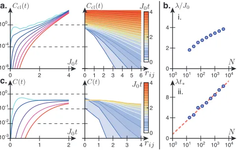
The growth in sensitivity Ccl(t) generically exhibits two distinct regimes [20], visible in Fig. 4. The first is a rapid power-law growth Ccl(t)∝(J0t)2rij forJ0t .1. A transition to exponential growth occurs for J0t & 1. Crucial to fast scrambling is that, by the time the expo-nential growth begins, the OTOCs have already reached valuesCcl∼1/Nα. We expect the subsequent exponen-tial growthCcl(t)∼eλt/Nα to yield a valueCcl(t∗)∼1
0 2 4
100
10-4
10-8
a. b.
0 1 2 3 4 5 6
0 1 2
100
10-2
10-1
10-3
0 1 2 3 4
0 4
2
0 4
2 c.
i.
104
103
102
101
100 ii.
104
2 4
0
103
102
101
100
4 8
[image:4.612.320.561.51.203.2]0
FIG. 4. Chaos and fast scrambling at s=0. (a) Average semiclassical sensitivityCcl(t) forN= 4096. (i)Cclvs. time
for graph distancesrij = 0,1, . . .6 (blue to red). (ii) Fixed-time contours ofCcl vs. rij, showing exponential decay of Ccl vs. rij at early times. Contours are for 0.2≤ J0t ≤4
in increments of 0.2. (b) Lyapunov exponent λ/J0 (i) and
scrambling timeλt∗ (ii) vs. N (blue circles) with fitλt∗ = αlog(N) +β(red dashed). (c) MPS calculations forN= 64, S= 1/2, and open boundary conditions.
at timet∗∼αlog(N)/λ. To verify this behavior, we first fit the exponential growth for a range of system sizes to obtain the dependence of the Lyapunov exponentλ on
N, and then evaluate the timet∗ to reachCcl(t∗) = 1 in terms ofλ(Fig. 4b). Fitting the dependence of this semi-classical scrambling time onN yieldsλt∗=αlog(N) +β, withα= 1.1(1).
Our semiclassical analysis demonstrates that the cor-relations developing at early times J0t . 1, before the onset of exponential growth, are crucial for enabling fast scrambling: the weakest correlations should be only alge-braically small (C ∝N−α) and not exponentially small inN. We now apply this insight to investigate whether the quantum model atS= 1/2 can be a fast scrambler.
As the essence of fast scrambling is efficient spread-ing of information across an exponentially large Hilbert space, the process is intrinsically difficult to study numer-ically. Nevertheless, we calculate the early-time dynam-ics forN = 64 sites at half filling using Matrix Product State (MPS) techniques [41, 57–61], for a system at in-finite temperature with open boundary conditions. We see no Lyapunov regime, which is not surprising since there is no small parameter forS = 1/2 at finite N to prevent rapid saturation of the OTOC (Fig. 4c). How-ever, Fig. 4c(ii) indicates early-time correlations that fall off exponentially with graph distancerij, consistent with correlations across all sites that are algebraically rather than exponentially small inN—the aforementioned nec-essary condition for fast scrambling.
the graph diameter grows logarithmically with system size. Near-term cavity-QED experiments offer promise for observing the logarithmic timescale for spin trans-port ats= 0, as well as the linear-to-treelike transition. In the large-Sregime, where each site contains an atomic ensemble, experiments will benefit from a collective en-hancement in the coherence of interactions. Ultimately, implementations of the spin-1/2 model—for sufficiently strong atom-light coupling [41, 62]—could test for fast scrambling [19, 41, 49, 50] at largeN ∼103in the quan-tum regime.
Complementarily, future theoretical work may investi-gate whether a Lyapunov regime can emerge in the spin-1/2 quantum model through a coarse-graining proce-dure that exploits the self-similarity of the coupling pat-tern. Measures of entanglement throughout the linear-to-treelike transition also merit further study, and may enable a more explicit connection to holography via en-tanglement wedges or tensor networks [22, 63–68]. Fu-ture work may also explore prospects for harnessing the rapid and deterministic generation of entanglement for quantum information processing.
This work was supported by the DOE Office of Sci-ence, Office of High Energy Physics. MS-S acknowledges support from the Research Corporation Cottrell Scholar Program and the NSF. SSG acknowledges support from the Simons Foundation. AJD, AB, and TH acknowledge support from the EPSRC Programme Grant DesOEQ (EP/P009565/1), and by the EOARD via AFOSR grant number FA9550-18-1-0064. We additionally acknowledge support from the NSF GRFP (EJD and GB) and Hertz Foundation (EJD), as well as support for international exchanges from SU2P. We thank Xiangyu Cao, Sean Hartnoll, Patrick Hayden, and Steve Shenker for help-ful discussions.
[1] Y. Sekino and L. Susskind, J. High Energy Phys.2008, 065 (2008).
[2] P. Hayden and J. Preskill, J. High Energy Phys.2007, 120 (2007).
[3] J. Maldacena, S. H. Shenker, and D. Stanford, J. High Energy Phys.2016, 106 (2016).
[4] J. Preskill, (2016), arXiv:1604.07450 [quant-ph]. [5] M. G¨arttner, J. G. Bohnet, A. Safavi-Naini, M. L. Wall,
J. J. Bollinger, and A. M. Rey, Nat. Phys.13, 781 (2017). [6] J. Li, R. Fan, H. Wang, B. Ye, B. Zeng, H. Zhai, X. Peng,
and J. Du, Phys. Rev. X 7, 031011 (2017).
[7] K. X. Wei, C. Ramanathan, and P. Cappellaro, Phys. Rev. Lett. 120, 070501 (2018).
[8] K. A. Landsman, C. Figgatt, T. Schuster, N. M. Linke, B. Yoshida, N. Y. Yao, and C. Monroe, Nature 567, 61 (2019).
[9] E. H. Lieb and D. W. Robinson, Comm. Math. Phys.28, 251 (1972).
[10] M. Cheneau, P. Barmettler, D. Poletti, M. Endres,
P. Schauß, T. Fukuhara, C. Gross, I. Bloch, C. Kollath, and S. Kuhr, Nature481, 484 (2012).
[11] P. Richerme, Z.-X. Gong, A. Lee, C. Senko, J. Smith, M. Foss-Feig, S. Michalakis, A. V. Gorshkov, and C. Monroe, Nature511, 198 (2014).
[12] S. Bravyi, M. B. Hastings, and F. Verstraete, Phys. Rev. Lett.97, 050401 (2006).
[13] M. B. Hastings and T. Koma, Commun. Math. Phys.
265, 781 (2006).
[14] M. Foss-Feig, Z.-X. Gong, C. W. Clark, and A. V. Gor-shkov, Phys. Rev. Lett.114, 157201 (2015).
[15] D. V. Else, F. Machado, C. Nayak, and N. Y. Yao, (2018), arXiv:1809.06369.
[16] I. Danshita, M. Hanada, and M. Tezuka, Prog. Theor. Exp. Phys.2017, 083I01 (2017).
[17] A. Chen, R. Ilan, F. de Juan, D. Pikulin, and M. Franz, Phys. Rev. Lett.121, 036403 (2018).
[18] A. Chew, A. Essin, and J. Alicea, Phys. Rev. B 96, 121119(R) (2017).
[19] B. Swingle, G. Bentsen, M. Schleier-Smith, and P. Hay-den, Phys. Rev. A94, 040302(R) (2016).
[20] J. Marino and A. Rey, Physical Review A99, 051803(R) (2019).
[21] S. S. Gubser, J. Knaute, S. Parikh, A. Samberg, and P. Witaszczyk, Commun. Math. Phys.352, 1019 (2017). [22] M. Heydeman, M. Marcolli, I. Saberi, and B. Stoica,
(2016), arXiv:1605.07639 [hep-th].
[23] J. L. F. Barb´on and J. M. Mag´an, J. High Energy Phys.
2012, 16 (2012).
[24] J. L. F. Barb´on and J. M. Mag´an, J. High Energy Phys.
2013, 163 (2013).
[25] C.-L. Hung, A. Gonz´alez-Tudela, J. I. Cirac, and H. Kimble, Proc. Natl. Acad. Sci. U.S.A. 113, E4946 (2016).
[26] S. Gopalakrishnan, B. L. Lev, and P. M. Goldbart, Na-ture Physics5, 845 (2009).
[27] I. D. Leroux, M. H. Schleier-Smith, and V. Vuletic, Phys. Rev. Lett.104, 073602 (2010).
[28] P. Strack and S. Sachdev, Phys. Rev. Lett.107, 277202 (2011).
[29] O. Hosten, R. Krishnakumar, N. J. Engelsen, and M. A. Kasevich, Science352, 1552 (2016).
[30] S. Welte, B. Hacker, S. Daiss, S. Ritter, and G. Rempe, Phys. Rev. X8, 011018 (2018).
[31] E. J. Davis, G. Bentsen, L. Homeier, T. Li, and M. H. Schleier-Smith, Phys. Rev. Lett.122, 010405 (2019). [32] R. M. Kroeze, Y. Guo, V. D. Vaidya, J. Keeling, and
B. L. Lev, Phys. Rev. Lett.121, 163601 (2018). [33] M. A. Norcia, R. J. Lewis-Swan, J. R. Cline, B. Zhu,
A. M. Rey, and J. K. Thompson, Science 361, 259 (2018).
[34] M. Landini, N. Dogra, K. Kroeger, L. Hruby, T. Donner, and T. Esslinger, Phys. Rev. Lett.120, 223602 (2018). [35] B. Braverman, A. Kawasaki, E. Pedrozo-Pe˜nafiel,
S. Colombo, C. Shu, Z. Li, E. Mendez, M. Yamoah, L. Salvi, D. Akamatsu, Y. Xiao, and V. Vuletic, (2019), arXiv:1901.10499.
[36] F. Borjans, X. G. Croot, X. Mi, M. J. Gullans, and J. R. Petta, (2019), arXiv:1905.00776.
[37] F. Mivehvar, H. Ritsch, and F. Piazza, Phys. Rev. Lett.
122, 113603 (2019).
[39] The tree appears to break translation invariance, but in fact it does not: dtree(i+ 1, j+ 1) =dtree(i, j).
[40] We thank P. Hayden for discussions on this point. [41] See Supplemental Material at [URL will be inserted by
publisher] for supporting derivations and additional ex-perimental details, including Refs. [42-43].
[42] J. J. Garc´ıa-Ripoll, New J. Phys.8, 305 (2006). [43] S. Paeckel, T. K¨ohler, A. Swoboda, S. R. Manmana,
U. Schollw¨ock, and C. Hubig, (2019), arXiv:1901.05824. [44] S. S. Gubser, C. Jepsen, Z. Ji, and B. Trundy, Phys.
Rev. D98, 045009 (2018).
[45] P. Weinberg and M. Bukov, SciPost Phys.2, 003 (2017). [46] S. Wimberger,Nonlinear Dynamics and Quantum Chaos
(Springer International Publishing, 2014).
[47] A. I. Larkin and Y. N. Ovchinnikov, Soviet Journal of Experimental and Theoretical Physics28, 1200 (1969). [48] S. H. Shenker and D. Stanford, J. High Energy Phys.
2014(2014), 10.1007/JHEP03(2014)067.
[49] B. Swingle and N. Yunger Halpern, Phys. Rev. A 97, 062113 (2018).
[50] Y.-L. Zhang, Y. Huang, and X. Chen, Phys. Rev. B99, 014303 (2019).
[51] G. Bentsen, Y. Gu, and A. Lucas, Proc. Natl. Acad. Sci. U.S.A.116, 6689 (2019).
[52] N. Lashkari, D. Stanford, M. Hastings, T. Osborne, and P. Hayden, J. High Energy Phys.2013, 22 (2013). [53] J. Maldacena and D. Stanford, Phys. Rev. D94, 106002
(2016).
[54] V. Khemani, D. A. Huse, and A. Nahum, Phys. Rev. B
98, 144304 (2018).
[55] A. Polkovnikov, Ann. Phys. (N. Y.)325, 1790 (2010). [56] J. S. Cotler, D. Ding, and G. R. Penington, Ann. Phys.
(N. Y.)396, 318 (2018).
[57] U. Schollwoeck, Ann. Phys. (N. Y.)326, 96 (2011). [58] J. Haegeman, J. I. Cirac, T. J. Osborne, I. Piˇzorn, H.
Ver-schelde, and F. Verstraete, Phys. Rev. Lett.107, 070601 (2011).
[59] T. Koffel, M. Lewenstein, and L. Tagliacozzo, Phys. Rev. Lett.109, 267203 (2012).
[60] J. Haegeman, T. J. Osborne, and F. Verstraete, Phys. Rev. B88, 075133 (2013).
[61] J. Haegeman, C. Lubich, I. Oseledets, B. Vandereycken, and F. Verstraete, Phys. Rev. B94, 165116 (2016). [62] Y. Colombe, T. Steinmetz, G. Dubois, F. Linke,
D. Hunger, and J. Reichel, Nature450, 272 (2007). [63] B. Swingle, (2012), arXiv:1209.3304.
[64] F. Pastawski, B. Yoshida, D. Harlow, and J. Preskill, J. High Energy Phys.2015, 149 (2015).
[65] A. Bhattacharyya, L.-Y. Hung, Y. Lei, and W. Li, J. High Energy Phys.2018, 139 (2018).
[66] M. Heydeman, M. Marcolli, S. Parikh, and I. Saberi, (2018), arXiv:1812.04057 [hep-th].
[67] G. Vidal, Phys. Rev. Lett.101, 110501 (2008).