Prognostics & health management methods & tools for transformer condition monitoring in smart grids

(1)

Advanced Research Workshop on Transformers (6)7 -9 October 2019 ARWtr2019 . Cordoba– Spain

Prognostics & Health Management

Methods & Tools for Transformer Condition Monitoring in Smart Grids

Jose Ignacio Aizpurua(1)_{, Brian G. Stewart}(2)_{, Stephen D. J. McArthur}(2)

Unai Garro(1)_{, Eñaut Muxika}(1)_{, Mikel Mendicute}(1)_{, V. M. Catterson}(3)_{, Ian P. Gilbert}(4)_{and Luis del Rio}(4)

(1)_{Signal Processing & Communications group, Electronics & Computer Science department, Mondragon University} 20500, Arrasate-Mondragon, Spain

+34678360304, e-mail: jiaizpurua@mondragon.edu, ugarro@mondragon.edu, emuxika@mondragon.edu, mmendikute@mondragon.edu

(2)_{Institute for Energy & Environment, Electronic & Electrical Engineering Department, University of Strathclyde} G1 1RD, Glasgow, United Kingdom

e-mail: brian.stewart.100@strath.ac.uk, s.mcarthur@strath.ac.uk (3)_BioSymetrics

Toronto, Canada e-mail: vic@ieee.org (4)_{Ormazabal Corporate Technology}

48340, Amorebieta, Spain

e-mail: igi@ormazabal.com, lre@ormazabal.com

Abstract — Condition monitoring of power transformers is crucial for the reliable and cost-effective operation of the power grid. The unexpected failure of a transformer can lead to different consequences ranging from a lack of export capability, with the corresponding economic penalties, to catastrophic failure, with the associated health, safety and economic effects. With the advance of prognostics and health management (PHM) applications, it is possible to enhance traditional transformer health monitoring techniques. Accordingly, this paper reviews the experience of the authors in the implementation of PHM methods for transformer condition monitoring and identifies research challenges in the use of PHM methods for transformer condition monitoring in smart grids.

Keywords — Data analytics, prognostics and health management, machine learning, transformer, smart grids.

1.INTRODUCTION

Transformers are complex assets comprised of different subsystems such as bushings, core, tank, cooler, oil preservation system, load tap changer, winding, and protection system [1]. Each of these subsystems performs a specific function (e.g., the cooler controls the oil temperature; the tap-changer regulates the voltage) and collectively, they determine the performance and health of the transformer. These dependencies can be formally represented through a Fault Tree Analysis (FTA) model which represents the combination of subsystem failures that can cause transformer failure. Fig. 1 shows a simplified transformer FTA model, where transformer subsystems and contributing failure modes are identified [1]. For example, the winding assembly failure can be caused by the failure of the winding, connector, or the insulation system, and in turn, the winding failure can be caused by turn-turn, coil-coil, or coil-ground faults.

(2)

The correct operation of the transformer depends on the correct operation of multiple related components over a variety of conditions. When monitoring the transformer’s health, the possible failure modes outlined in Fig. 1 need to be examined.

Traditional methods for transformer health assessment have been focused on the analysis of, e.g. gases dissolved in oil, temperature, or electrical parameters. The estimation of their remaining useful life (RUL) can be done through deterministic lifetime models based on IEEE standards [2] that may lead to conservative lifetime management strategies. There are other asset management models, which combine the information of different subsystems to elicit a health index value of the transformer, e.g. [3], [4].

The use of deterministic lifetime models may be appropriate for transformer lifetime planning if they are operated with regular power and temperature profiles. However, if the application context includes dynamic operation profiles and stochastic phenomena, the transformer health state estimation is no longer deterministic and new health state estimation models are needed [5]. This is the case of transformers operated within smart grids [6], where the lifetime estimation is further complicated due to the random and dynamic nature of the connected technologies such as renewable generation or electric vehicles. For example, it is common to use numerical weather prediction models to estimate the power generation in a renewable power plant, and accordingly, it is necessary to use stochastic power prediction profiles for transformer lifetime planning.

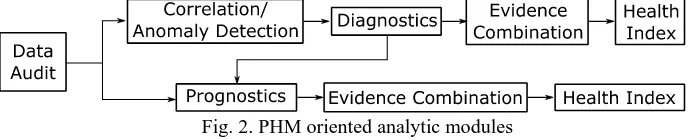
[image:2.595.126.470.342.412.2]

With the advance of prognostics and health management applications (PHM), traditional transformer health monitoring techniques can be enhanced with PHM analytics that include anomaly detection, diagnostics or prognostics analysis modules [7]. For a consistent design of PHM analytic modules, a multi-stage design methodology is needed. Fig. 2 shows the logical flow of the PHM-oriented design methodology [7].

Fig. 2. PHM oriented analytic modules

The PHM analytics design process starts from the data audit step by listing available datasets and identifying new variables that can be monitored to improve the health assessment process. Next the correlation and anomaly

detection are implemented so as to identify abnormal data patterns. If an anomalous data trend is detected, then the diagnostics follows the process for the identification of failures. The evidence combination aims to combine different diagnostics outcomes to generate an overall transformer diagnosis. Similarly, the health index generates an overall transformer health state indicator combining the information generated in all the previous activities. After diagnosing the current health, it is possible to implement prognostics methods to estimate the remaining useful life (RUL) through the application of future profiles. As with the diagnostics state, it is possible to implement evidence combination and health index activities so as to generate a single consistent RUL estimation.

Following the design methodology outlined in Fig. 2, this paper presents a review of different PHM applications for condition monitoring of transformers and discusses the future applications that can emerge in the context of condition monitoring in smart grids. Refer to [4] or [7] for more details about the implementation of the methodology in Fig. 2 through a data analytics framework. The remainder of this paper is organised as follows. Section 2 presents a conditional anomaly detection module for power transformers. Section 3 focuses on transformer fault diagnostics models through dissolved gas analysis techniques. Section 4 presents prognostics techniques for transformer lifetime prediction. Section 5 presents a lifetime estimation framework for transformers operated in smart grids, and finally Section 6 draws conclusions.

2.ANOMALY DETECTION

(3)

In this context, one alternative is to implement a conditional anomaly detection (CAD) model [7], [8], which correlates the internal condition-related data of the transformer and external operational data. Fig. 3 shows the CAD model implemented for the transformer.

The goal of the CAD module is to distinguish situations where unusual operating conditions may be causing abnormal transformer behaviour from situations where the transformer condition is unusual under normal operation. The latter case is more likely to represent a true deterioration of the health of the transformer.

Fig. 3. Transformer conditional anomaly detection model.

In order to implement the CAD model, Gaussian Mixture Models are used which generate multivariate Gaussian distributions that embed condition-related data within a transformer model, P(Transf), and operating environment related data within an environment model, P(Env). The set of Gaussian components and their mixing proportions constitute a probabilistic model of the dataset. Then a correlation algorithm is used to generate a conditional probability model that correlates the environment and transformer models, P(Transf |

Env), i.e. Expectation Maximization (EM) algorithm [7], [8]. EM converges towards a locally optimal set of values that maximize the likelihood of the model P(Transf | Env).

The CAD module can take multiple different input variables to the transformer and environment models. For example, as shown in Fig. 3, gas parameters can generate the transformer model (e.g., CH4, C2H6) and

temperature and load parameters the environment model. The CAD module will identify truly anomalous trends under normal operating conditions, and when combined with the diagnostics activity, it will reduce false alarms by triggering the diagnosis activity only if an anomaly has been identified.

The development of the CAD model requires training environment and transformer models, and then generating a correlation model. In this case, as an illustrative example, the generated power and ambient temperature have been used in the environmental model, and methane (CH4) and hydrogen (H2) for the

transformer model (see also Fig. 3). Both models have been trained based on normal operation data, which is determined by a period of stable gas levels, and the rest of data is used for testing (20 samples).

Fig. 4a shows the trained environment model, where the axes in the horizontal plane denote normalized training values of true power and temperature and the vertical axis identifies their joint probability density, e.g. when the true power is very high it is likely that the temperature will be low. Fig. 4b shows the trained transformer model where horizontal plane axes denote methane and hydrogen, and the vertical axis denotes the probability density, e.g. it is very likely that when hydrogen is small methane is small too. These figures model the expected independent normal behaviour of the transformer and environment.

[image:3.595.117.478.563.737.2]

(4)

After learning the environment and transformer models, the correlation models are tested. Fig. 4c shows the normalized test data and Fig. 4d shows the CAD outcome, where the red horizontal line identifies the failure threshold and the vertical dashed line indicates the division between training and testing data.

It is possible to see in Fig. 4d that almost all the test data is classified as anomalous because the environment probability is high (triangles above the red line: normal environment), but the transformer model’s probability is low (squares below the red line), which indicates a true anomaly (circles below the red line). Note also that the last sample is classified as healthy (circle in the top right) because both transformer and environment models match with the trained models (Figs. 4a and 4b).

In this particular case, the gas levels from the test period were known to be significantly different from those during the training period. This resulted from a scheduled change in operation of the cooling of the transformer, and the gassing behaviour was being carefully monitored. Therefore, this case shows the power of the CAD technique to recognize anomalous behaviour.

3.DIAGNOSTICS

Operational and fault events generate gases which are dissolved in the oil that circulates through a transformer for cooling and insulation purposes. Dissolved Gas Analysis (DGA) is a mature and industry-standard method that focuses on the study of these gases [9].

There are different industry-accepted classical DGA methods including Duval’s triangle, Roger’s ratios, or Doernenburg’s ratios [9]. These techniques classify transformer faults based on the predefined range of specific fault gas ratios. However, their accuracy is limited because they assume crisp, deterministic decision bounds [10]. This leads to a decreased diagnostics accuracy and conflicting diagnostics outcomes among methods which do not help engineers in the decision-making process. From an engineering viewpoint, the disagreements among independent classifiers are the most important situations thatneed to be resolved effectively because conflicting diagnoses may imply very different maintenance actions. Therefore, it is critical to analyse and quantify the strength of classifiersin the presence of conflicting data.

So as to improve the classification accuracy a number of machine learning models have been proposed. Most of these algorithms have been focused on solving a supervised learning problem. That is, usinga DGA dataset comprised of n samples, 𝐷𝐺𝐴 = {𝑥_𝑖, 𝑦_𝑖}𝑛_𝑖=1, where the pair {𝑥_𝑖, 𝑦_𝑖} contains the data related to the i-th observation, 𝑥_𝑖 ∈ 𝑋 and 𝑦_𝑖 ∈ 𝑌. The matrix 𝑋 ∈ ℝ𝑛𝑥𝑝 contains the information 𝑋 = {𝑥₁, … , 𝑥_𝑛} for p fault gases, and the vector 𝑌 ∈ ℝ𝑛𝑥1_{contains the information about the health state of the transformer.}

In a binary classification problem the set of possible states of 𝑦_𝑖 are limited to normal and fault states. However, in this case, there are multiple states and the transformer state can be classified as: normal degradation, thermal fault, arc fault, and PD. Therefore, each output 𝑦_𝑖 can take the following values: 𝑦_𝑖 = {𝑛𝑜𝑟𝑚𝑎𝑙, 𝑡ℎ𝑒𝑟𝑚𝑎𝑙, 𝑎𝑟𝑐, 𝑃𝐷}. Multiclass classification problems are more challenging than binary classification problems, but they also generate more useful information for maintenance planning.

In this section black-box (BB) and white box (WB) source classifiers will be tested for DGA diagnostics and then a fusion strategy will be implemented to combine the outcome of different source classifiers. BB models generally show a high classification accuracy, but their usability for resolving misclassified data samples is limited because their diagnostics is deterministic and they do not generate uncertainty information. WB models capture expert knowledge either as a causal model or through first-principle models. They generate the uncertainty associated with the decision-making process by quantifying the PDF of the likelihood of different diagnostics states.

ANN and SVM models will be used as BB classification models as they have shown a high accuracy on DGA data [10]. For WB modelling Gaussian Bayesian networks (GBNs) will be used because they are able to capture the causality among random variables (RVs) and infer uncertainty information [10].

Artificial Neural Networks (ANNs)

(5)

through an activation function. All the designed ANN models use a sigmoid activation function for hidden and output nodes.

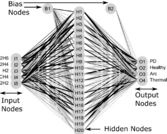
Model training is performed using a back-propagation algorithm. The goal is to learn the neuron weights to generate the transformer health state (network output) from DGA values (sample input), which minimizes the error with respect to the target transformer health state. Of the trained networks for each trial, the one with the highest mean accuracy was selected. For most of the trials best results were obtained with 20 hidden nodes with the inputs in Fig. 5, i.e., C2H6, C2H4, H2, CH4, and C2H2.

[image:5.595.223.389.197.331.2]

Fig. 5 also shows the strength of the neuron weights with a black line for higher weights and a gray line for lower weights. Model training was performed using the R nnet library [12].

Fig. 5. ANN configuration.

Support Vector Machines (SVMs)

The SVM maps input data into a space using a kernel function [13]. The SVM learns the boundary separating one transformer health state from another with maximum distance. The kernel function aims to translate a problem that is nonlinearly separable into a feature space, which is linearly separable by a hyperplane. The hyperplane represents the transformer health state classification boundary.

The SVM is parametrized through the choice of kernel function. For a nonlinear problem, such as the transformer health state estimation, the RBF kernel is recommended [13]: 𝑘(𝑥, 𝑥′_{) = 𝑒𝑥𝑝(−𝛾||𝑥 − 𝑥}′_||2₎_{, where} 𝛾 is the RBF width, 𝑥 and 𝑥′ are training and testing data samples, and ||d|| is the Euclidean norm. The SVM solves an optimization problem maximizing the distance from the transformer health classification hyperplane to the nearest DGA training point. Generally, the dataset is not linearly separable and slack variables are used to allow wrongly classified samples. SVM penalizes the objective function with a cost variable c, which is a trade-off between penalizing slack variables and obtaining a large margin for the SVM.

Therefore, the SVM training consists of calculating thehyper-parameters c and 𝛾. Grid search was used to find theoptimal parameters of c and 𝛾from a grid of values. Namely, for each trial, model training was performed using the R e1071package [14] and grid searchwas used to optimize c and 𝛾within c = [2-10, 210] and𝛾 = [22,

29]. A number of configurations were trained usingall different gases and their ratios as input to the SVM. Of thetrained SVMs, the one with the highest accuracy from the testdata was selected as the choice for that output, which matcheswith the input data used for the ANN model: C2H6, C2H4, H2, CH4 and C2H2.

Gaussian Bayesian Networks (GBN)

Bayesian networks (BN) [15] are statistical models that capture probabilisticdependencies among random variables. Graphically, thesevariables are represented through nodes and they are linkedthrough edges to reflect dependencies between variables.Statistically, dependencies are quantified through conditionalprobabilities. BNs are a compact representation of jointprobability distributions. In probability theory, the chain rule permits the calculation of any member of the joint distributionof a set of random variables using conditional probabilities.

(6)

[image:6.595.232.358.134.239.2]

linked through linear models in which the parents play the role of explanatory variables. Each node 𝑥_𝑖 is regressed over its parent nodes. Assuming that the parents of 𝑥_𝑖 are {𝑢₁, … , 𝑢_𝑘} then the conditional probability of each node can be expressed as 𝑝(𝑥𝑖|𝑢1, … , 𝑢𝑘)~𝑁(𝛽0+ 𝛽0𝑢1+ ⋯ + 𝛽𝑘𝑢𝑘; 𝜎2), where 𝛽0 is the intercept and {𝛽₁, … , 𝛽_𝑘} are linear regression coefficients for the parent nodes {𝑢₁, … , 𝑢_𝑘}. Fig. 6 shows the GBN model.

Fig. 6. GBN configuration.

The parameter estimation for GBN models is based on the maximum likelihood algorithm which estimates the corresponding parameters for each node in the BN model, e.g. for the Arc node (Fig. 6):

𝑃𝑟(𝐴𝑟𝑐|𝐶₂𝐻₆, 𝐶₂𝐻₂, 𝐶𝐻₄, 𝐶₂𝐻₄, 𝐻₂)~𝑁(𝛽0+ 𝛽1𝐶2𝐻6+ 𝛽2𝐶2𝐻2+ 𝛽3𝐶𝐻4+ 𝛽4𝐶2𝐻4+ 𝛽5𝐻2; 𝜎2).

After learning the parameters, the estimation of the conditional probability of nodes is based on inferences. In this case, the likelihood weighting algorithm is implemented, which fixes the test DGA gas samples (evidence) and uses the likelihood of the evidence to weight samples [15]. When applied to the DGA dataset, for each of the analyzed faults the outcome of the inference is a set of random samples from theconditional distribution of the fault node given the evidence.

Density values of the inference outcomes can be calculated through Kernel density estimates [16]. The GBN model was implemented using the bnlearn R package [17].

Fusion of Classifiers via Dempster Shafer’s Theory

In order to avoid conflicting outcomes it is possible to combine the outcome of source classifiers through evidence combination strategies. This paper implements Dempster Shafer (DS) theory for information fusion tasks [18], but note that there are other methods, which can be used for the same task such as weighted average or more complex fusion strategies, e.g. see [10].

DS builds beliefs of the true state of a process from distinct pieces of evidence, e.g. [19]. Assuming a set of faults 𝐹 = {𝑓₁, … , 𝑓_𝑖, … , 𝑓_|𝐹|} the set of possible states is called the frame of discernment, F. Pieces of evidence are formulated as mass functions, m, satisfying: m(fi)≥0, m()=0, and ∑_𝑓_𝑖_⊆𝐹𝑚(𝑓_𝑖) = 1.

The combined probability mass for the i-th fault, fi, of two classifiers, denoted c1 and c2, is defined as:

𝑚_𝑐1𝑐2(𝑓_𝑖) = 1

1 − 𝐾 ∑ 𝑚𝑐1(𝐴)𝑚𝑐2(𝐵)

𝐴,𝐵⊆𝑓

𝐴∩𝐵=𝑓𝑖

(1)

 fi  F, fi=  , where K is the degree of conflict between two mass functions:

𝐾 = ∑ 𝑚_𝑐1(𝐴)𝑚𝑐2(𝐵)

𝐴,𝐵⊆𝑓

𝐴∩𝐵=𝑓_𝑖

(2)

Performance Results

(7)

[image:7.595.125.471.73.118.2]

Table I. Classification accuracy results.

Method GBN ANN SVM DS Fusion

Accuracy 81.9 % ± 6.5% 89.4 % ± 5.1% 86.3 % ± 5.9% 90.1 % ± 5.3%

It can be seen from Table I that the Dempster Shafer’s fusion strategy is the most accurate diagnostics method. Among the source classifiers ANN shows the best accuracy with respect to the other classifiers.

It is interesting to observe that the accuracy of the GBN model is not as high as SVM and ANN models, but the information inferred from the outcome of GBN models is more useful. For instance, consider that after training the source classifiers, they are tested for the following absolute gas values [10]: H2 = 26788 ppm, C2H4

= 27 ppm, C2H6 = 2111 ppm, C2H2 = 1 ppm, and CH4 = 18342 ppm and the observed fault type is partial

[image:7.595.165.431.266.360.2]

discharge. Table II displays probabilistic results for the different classifiers and for the different possible health states of the transformer, i.e. normal degradation, thermal fault, arcing fault and partial discharge fault.

Table II. Classification accuracy results.

Method Pr(Normal) Pr(Thermal) Pr(Arc) Pr(PD)

GBN 0.23 0.28 0.18 0.31

SVM 0.08 0.45 0.07 0.4

ANN 3.9E-2 0.5 4.8E-6 0.46

ANN and SVM models do not generate more information other than shown in Table II. However, GBN models generate PDFs with uncertainty information as shown in Fig. 7. If the designed GBN model is confident about the diagnostics output it will generate a PDF with a narrow standard deviation, i.e. PD fault. In contrast, for uncertain diagnostics outcomes the generated PDFs are wider with greater standard deviation values, e.g. Normal degradation.

Fig. 7. GBN output example.

So long as the test data is comprised of faults which are similar to the trained model, the trained GBN model should return a prediction with high confidence. However, if the model is tested on an unseen class of fault, the model should be able to quantify this with uncertainty levels which can convey information about the confidence of the diagnosis of the model. This uncertainty information can be used to further post-process the results and improve the diagnostics accuracy. Interested readers please refer to [10] for more information on uncertainty post-processing for improved transformer diagnostics.

4.PROGNOSTICS

The IEEE standard C57.91 defines the insulation paper aging acceleration factor at time t, 𝐹_𝐴𝐴(𝑡), as [2]:

𝐹𝐴𝐴(𝑡) = 𝑒 15000

383 − 15000

273+𝜃𝐻(𝑡) (3)

(8)

𝜃_𝐻(𝑡) = 𝜃𝑇𝑂(𝑡) + ∆𝜃𝑇𝑂,𝐻(𝑡) (4)

where 𝜃_𝑇𝑂(𝑡) is the top oil (TO) temperature at time instant t and ∆𝜃_{𝑇𝑂,𝐻}(𝑡) is the hottest-spot temperature rise over top oil temperature at time instant t.

The hottest-spot temperature in (2) is inferred from other measurements and these measurements may include measurement errors that may affect the hottest-spot temperature estimation accuracy. Assuming steady-state measurements and including measurement errors, the hottest-spot temperature can be calculated as follows [5]:

𝜃𝐻(𝑡) = (𝜃𝑇𝑂(𝑡) + 𝜑𝑇𝑂) + ∆𝜃𝐻,𝑅[(𝑖(𝑡) + 𝜑𝑖)/𝑖𝑅]2𝑚 (5)

where 𝑖(𝑡) is the transformer load at time t, 𝑖𝑅is the rated load, ∆𝜃𝐻,𝑅 is the hottest-spot temperature rise at rated

load, m is a transformer parameter determined from a lookup table depending on the cooling system of the transformer [5], 𝜑_𝑇𝑂 denotes the top oil measurement error and 𝜑_𝑖 designates the load measurement error.

The degradation process of the insulation paper is not a deterministic process and it needs to integrate sources of uncertainty corresponding to the degradation process [5]:

𝑅𝑈𝐿(𝑡) = 𝑅𝑈𝐿(𝑡 − 1) + 𝜔𝑅𝑈𝐿𝑡−1− 𝑒

(15000+𝜔𝑡)(₃₈₃1−_273+𝜃1

𝐻(𝑡)) (6)

where 𝜔_𝑡 denotes the degradation process uncertainty due to the lack of exact knowledge at time instant t, 𝜔_𝑅𝑈𝐿_𝑡−1

denotes the uncertainty of the lifetime estimation at time instant t-1, and 𝜃_𝐻(𝑡) is defined in (3). Initially 𝜔_𝑅𝑈𝐿_𝑡−1

will denote the initial lifetime estimation error, 𝜔_𝑅𝑈𝐿₀. This error will be propagated and updated in subsequent iterations through the recurrence relation form of the RUL estimation in (4).

Top Oil Temperature Forecasting

[image:8.595.102.512.506.617.2]

The hottest-spot temperature is inferred from indirect measurement such as top-oil temperature, ambient temperature and load as defined in Eq. (5). Given an input load profile and other influencing parameters, it is possible to design a top-oil temperature forecasting model which can then be used to estimate the hottest-spot temperature. Fig. 8 shows load, ambient temperature, water temperature and top-oil temperature measurements hourly sampled for a period of 3 years and 10 months.

Fig. 8. Load, water temperature, ambient temperature and top oil temperature datasets [5].

It can be seen that the top-oil temperature profile in Fig. 8 is non-linear. Additionally, depending on the harshness of the winter, loadconditions and applied water temperature, the oil temperaturecan drop below zero degrees, e.g. winter 2016.

There are different forecasting methods that can be used to estimate the top-oil temperature, e.g. see [5] for a review. In this case, extreme gradient boosting (XGB) has been selected as a forecasting model due to its forecasting abilities [20]. XGB is a faster and more efficient implementation of gradient boosting, which creates an accurate learner by combining many regression trees. The objective of training an XGB model is to minimize the training loss and avoid overfitting through regularization terms. This process is based on additive training implemented through a second order gradient algorithm [20].

(9)

forecasting error. Feature selection and processing steps will not be covered here, but refer to, e.g. [5], for an extended discussion on the area. The XGB model has been implemented through the xgbtree package in R [20]. The hyperparameters include the maximum depth of the tree (max depth) and learning rate (η). The more complex the tree, the more complicated patterns it will learn, but it will be more prone to over-fitting. The learning rate models the error generalization.

These hyperparameters have been optimized through a 10 repeated 5 fold cross validation process searching the optimal parameters from a predefined grid of parameters: η=[0.001, 0.003, 0.01, 0.1, 0.3], max depth=[1, 2, 4, 6, 10]. Namely, the available datasets are divided into 5 equidistant folds. Then a XGB model is trained for the first fold and tested with the second fold, subsequently the same model is trained with the first two folds and tested with the third fold and the validation continues until the last step, where the models are trained with the first four folds and tested on the last fold. The best parameters for this work are η=0.3 and maxdepth=2.

Table II displays the forecasting results using the XGB model and the IEEE standard C57.91. Table II demonstrates that the XGB obtains a more accurate diagnostics accuracy than the IEEE model.

Table II. Top oil temperature forecasting results.

Tech. Fold 1 Fold 2 Fold 3 Fold 4 Average

XGB 4.13±0.28 5.07±0.35 6.63±0.67 9.1±0.15 6.23±2.17

IEEE C57.91 5 5.6 8.6 12 7.77±3.2

Lifetime Estimation Framework

[image:9.595.115.490.393.455.2]

This section defines the high-level solid insulation lifetime prediction framework. Fig. 9 shows the block diagram of the transformer lifetime prediction framework.

Fig. 9. Lifetime estimation framework.

As discussed in the previous section, after pre-processing and extracting features from the inspection data, the XGB model predicts the top-oil temperature. Then, using Eqs. (5) and (6), the Particle Filter model is implemented which estimates the RUL of the transformer’s solid insulation integrating and propagating multiple sources of uncertainty present in the lifetime estimation process [5].

[image:9.595.210.408.559.677.2]

Three different scenarios have been tested taking as input hypothetical water, ambient temperature profiles, and the load profiles shown in Fig. 10.

Fig. 10. Load and temperature test data.

Firstly, the top-oil temperature, 𝜃̂TO, is estimated from the scenarios shown in Fig. 10. Subsequently, this is used to estimate the hottest-spot temperature, 𝜃̂HST, and in the end the lifetime estimation, RUL.

(10)

[image:10.595.202.416.62.175.2]

Fig. 11. RUL estimations.

The RUL estimates in Fig. 11 are in agreement with the applied load profiles in Fig. 10. That is, profile C shows the greatest RUL reduction while profile A shows the least RUL prediction.

5.PROBABILISTIC HEALTH INDEX FOR TRANSFORMERS OPERATED IN SMART GRIDS

The different technologies present in smart grids generate dynamics and sources of uncertainty that affect the lifetime planning of transformers operated in smart grids. For example, wind energy prediction models, which are an integral part for power generation planning, make use of numerical weather prediction models for wind speed forecasting of individual wind turbines. Subsequently, individual wind turbine predictions are aggregated for the estimation of the generated power at wind farm level. This power estimation process includes different sources of uncertainty at wind turbine and wind farm levels and the generated power directly affects the current flowing through the transformer. In parallel, the current that flows through the transformer directly influences the temperature of the solid insulation and accordingly the transformer RUL estimation. This example can be extended to other renewable energy sources and low carbon technologies, such as solar energy applications or electric vehicles, which are driven by uncertainty-surrounded technologies and operation contexts.

In this context, it is necessary to integrate and propagate different dynamics and sources of uncertainty for an accurate transformer health state estimation. Fig. 12 shows the high-level framework for condition monitoring of transformers operated in smart grids.

Fig. 12. Generic framework for transformer condition monitoring in smart grids.

Transformer subsystems are influenced by the different dynamics and sources of uncertainty emerging from smart grids, which in the end affects the overall transformer health. The estimation of the effect of uncertainty for the different transformer subsystems along with their integration for a consistent transformer health index specification is an ongoing research challenge [3]-[6]. The effective health index implementation should integrate the influence and interactions of different subsystems.

Focusing on the solid insulation health state estimation, it is possible to adapt the lifetime modelling framework in Fig. 12 so as to take into account possible probabilistic forecasting models and their results, which can come from, e.g. wind or solar energy prediction models. Probabilistic forecasting models which can generate probability density function (PDF) based forecasts are of special interest due to their capability to integrate and propagate uncertainties. PDFs represent a probabilistic interpretation of the different possible forecasting estimates. In addition to the PDF-based forecasts, methodologies that can integrate different sources of uncertainty are also necessary which would allow the health state estimation under uncertainty with the consideration of the different sources of uncertainty.

[image:10.595.121.473.422.552.2]

(11)

[image:11.595.119.474.95.197.2]

integrate and propagate different sources of uncertainty through their corresponding PDF estimates.

Fig. 13. Solid insulation RUL estimation framework.

The probabilistic thermal model estimates the PDF of the top-oil temperature, 𝑝𝑑𝑓̂ (𝑡)_𝜃_𝑇𝑂, and the PDF of the solid insulation’s hottest-spot temperature, 𝑝𝑑𝑓̂ (𝑡)_𝜃_𝐻𝑆𝑇, through statistical and expert based modelling strategies, respectively. The probabilistic lifetime modelling framework is based on the implementation of the IEEE lifetime model in [2] through the Particle Filtering approach [5] to integrate previous forecasting results and different sources of uncertainty in the IEEE lifetime model. Refer to the example in [21] for more details about the proposed forecasting approach and the technical implementation.

The example framework in Fig. 13 can be adapted to different forecasting strategies. For example, if the prediction of the car traffic influences the health state of the battery of the cars, and accordingly this impacts on the battery charging profile, which is associated with the current that flows through the transformer, a similar RUL and lifetime estimation strategy can be implemented.

Fig. 13 shows a possibility to integrate the effect of forecasting models on transformer insulation lifetime estimation. The same task should be performed with other transformer subsystems by analysing the influencing factors and the sources of uncertainty as well as the interactions among different transformer subsystems. In the end, the integration and propagation of the different sources of uncertainty adds the capability to adapt the health index and the associated confidence intervals according to the different dynamics and sources of uncertainty that impact on the transformer lifetime.

Novel energy generation, consumption and storage applications emerging in the context of smart grids lead to an increase in the sources of uncertainty that affect the transformer operation conditions. In this direction, the generic transformer condition monitoring framework shown in Fig. 12 highlights the need to integrate and propagate the different dynamics and sources of uncertainty for an accurate transformer health state estimation.

6.CONCLUSIONS

This paper has presented a number of prognostics and health management applications for transformer condition monitoring. Namely, the implementation details for the implementation of anomaly detection, diagnostics and prognostics applications have been described. Most of the presented techniques combine data-driven machine learning methods with expert knowledge based strategies with a special emphasis on uncertainty processing for an improved performance in operation contexts with various sources of uncertainty.

With the emerging challenges arising from smart grids and the associated technologies, research directions have been discussed for the effective condition monitoring of transformers operated in smart grids.

REFERENCES

[1] IEEE Guide for the Evaluation and Reconditioning of Liquid Immersed Power Transformers, IEEE standard C57.140,

2006.

[2] IEEE Guide for Loading Mineral Oil Immersed Transformers and Step Voltage Regulators, IEEE standard C57.91,

2011.

[3] A. Azmi, J. Jasni, N. Azis, and A. Kadir, Evolution of transformer health index in the form of mathematical equation, Renewable & Sustainable Energy Reviews, vol. 76, pp. 687-700, 2017.

(12)

[5] J. I. Aizpurua, B. G. Stewart, S. D. J. McArthur, B. Lambert, J. Cross and V. M. Catterson, Adaptive Power Transformer Lifetime Predictions through Machine Learning & Uncertainty Modelling in Nuclear Power Plants, IEEE Transactions on Industrial Electronics, vol. 66, no. 6, pp 4726-4737, 2019.

[6] M. Liserre, G. Buticchi, M. Andersen, G. Carne, L. Costa and Z. Zou, The Smart Transformer: Impact on the Electric Grid and Technology Challenges, IEEE Industrial Electronics Magazine, vol. 10, no. 2, pp 46-58, 2016.

[7] J. I. Aizpurua, V. M. Catterson, B. G. Stewart, S. D. J. McArthur, B. Lambert, B. Ampofo, G. Pereira and J. Cross,

Determining appropriate data analytics for transformer health monitoring, In proceedings of NPIC & HMIT 2017,

San Francisco, 2017.

[8] V. M. Catterson, S. D. J. McArthur and G. Moss, Online Conditional Anomaly Detection in Multivariate Data for

Transformer Monitoring, IEEE Transactions on Power Delivery, vol. 24, no. 4, October 2010.

[9] IEEE Guide for the Interpretation of Gases Generated in Oil-Immersed Transformers, IEEE standard C57.104, 2009.

[10] J. I. Aizpurua, V. M. Catterson, B. G. Stewart, S. D. J. McArthur, B. Lambert and J. Cross, Uncertainty-Aware Fusion of Probabilistic Classifiers for Improved Transformer Diagnostics, IEEE Transactions on Systems Man and Cybernetics: Systems, In Press, 2019.

[11] M. R. G. Meireles, P. E. M. Almeida, and M. G. Simoes, A comprehensive review for industrial applicability of artificial neural networks, IEEE Transactions on Industrial Electronics, vol. 50, no. 3, pp. 585–601, Jun. 2003 [12] R B. Ripley, W. Venables and M. B. Ripley, Package ‘nnet’, R package version, 7, 3-12, 2016.

[13] A. J. Smola and B. Scholkopf, A tutorial on support vector regression, Statistics and Computing, vol. 14, no. 3, pp. 199–222, Aug. 2004.

[14] R E. Dimitriadou, K. Hornik, F. Leisch, D. Meyer, and A. Weingessel, Misc Functions of the Department of Statistics (e1071), R Package 1.5–24, TU Wien, Vienna, Austria, 2008

[15] R. E. Neapolitan, Learning Bayesian Networks. Upper Saddle River, NJ, USA: Prentice-Hall, 2004

[16] K. J. Seuk and C. Scott, Robust Kernel Density Estimation, In Proceedings of the IEEE Int. Conference on Acoustics, Speech and Signal Processing, pp. 3381-3384, 2008.

[17] M. Scutari, Learning Bayesian networks with the bnlearn R package, Journal of Statistical Software, vol. 35, no. 3, pp. 1–22, 2010.

[18] D. Fixsen and R. P. S. Mahler, The Modified Dempster–Shafer Approach to Classification, IEEE Transactions on Systems, Man and Cybernetics. Part A: Systems & Humans, vol. 27, no. 1, pp. 96–104, Jan. 1997.

[19] D. Bhalla, R. K. Bansal, and H. O. Gupta, Integrating AI based DGA Fault Diagnosis using Dempster–Shafer Theory, International Journal of Electric Power & Energy Systems, vol. 48, pp. 31–38, Jun. 2013

[20] T. Chen and C. Guestrin, Xgboost: A scalable tree boosting system, In Proceedings of ACM Knowledge Discovery & Data Mining, pp. 785–794, 2016.