Research Article
Weakly Supervised Deep Semantic Segmentation Using CNN and
ELM with Semantic Candidate Regions
Xinying Xu,
1Guiqing Li,
1Gang Xie ,
1,2Jinchang Ren ,
1,3and Xinlin Xie
11College of Electrical and Power Engineering, Taiyuan University of Technology, Taiyuan, China
2College of Electronic Information Engineering, Taiyuan University of Science and Technology, Taiyuan, China 3University of Strathclyde, Department of Electronic and Electrical Engineering, Glasgow, UK
Correspondence should be addressed to Gang Xie; [email protected] and Jinchang Ren; [email protected]
Received 15 November 2018; Revised 3 February 2019; Accepted 25 February 2019; Published 14 March 2019
Guest Editor: Jungong Han
Copyright © 2019 Xinying Xu et al. This is an open access article distributed under the Creative Commons Attribution License, which permits unrestricted use, distribution, and reproduction in any medium, provided the original work is properly cited.
The task of semantic segmentation is to obtain strong pixel-level annotations for each pixel in the image. For fully supervised semantic segmentation, the task is achieved by a segmentation model trained using level annotations. However, the pixel-level annotation process is very expensive and time-consuming. To reduce the cost, the paper proposes a semantic candidate regions trained extreme learning machine (ELM) method with image-level labels to achieve pixel-level labels mapping. In this work, the paper casts the pixel mapping problem into a candidate region semantic inference problem. Specifically, after segmenting each image into a set of superpixels, superpixels are automatically combined to achieve segmentation of candidate region according to the number of image-level labels. Semantic inference of candidate regions is realized based on the relationship and neighborhood rough set associated with semantic labels. Finally, the paper trains the ELM using the candidate regions of the inferred labels to classify the test candidate regions. The experiment is verified on the MSRC dataset and PASCAL VOC 2012, which are popularly used in semantic segmentation. The experimental results show that the proposed method outperforms several state-of-the-art approaches for deep semantic segmentation.
1. Introduction
Image semantic segmentation is the understanding of the semantic information contained in images. It uses the com-puter to extract semantic information of the captured scene from the image for understanding its contents, which can be applied in image recognition, classification, and analysis [1]. Semantic segmentation has been widely used in intelli-gent robot scene understanding, automatic driving system streetscape recognition, and medical image detection [2]. However, semantic segmentation has become one of the most challenging computer vision tasks due to the scale, position, illumination, and texture changes of objects in the image [3].
In most cases, image semantic segmentation is established as a fully supervised task. The fully supervised methods require using strong pixel-level annotations, which is very limited, expensive, and time-consuming in the labeling pro-cess, and it is different due to the subjective understanding
of the labeling personnel [4]. However, weakly supervised semantic segmentation only requires image labels at the image-level, which is much cheaper and less time-consuming than pixel-level annotations. Weakly supervised semantic segmentation can be divided into three categories that included bounding box [5], partial marking [6], and image-level labels. At present, with the increasing popularity of image sharing websites (for example, Flickr) and providing a large number of user-labeled images, many studies have focused on image-level labels for weakly supervised semantic segmentation.
Therefore, the semantic segmentation of weakly super-vised images based on image-level labels has gradually increased recently. According to the different methods of semantic label inference, the weakly supervised image semantic segmentation can be roughly divided into clas-sifier, multigraph model, and deep convolutional neural network based methods. Among them, the first classifier-based method uses the superpixels or the candidate regions
Data set
Candidate region
grass
sky
aeroplane
…
Candidate region
with labels
Neighborhood rough set
segmentation image
with semantic SLIC
Superpixel
merging
ELM
1 i L
1 n
Semantic associated
relationship
building
sky
tree grass
cow sheep
road
car i
1 L
xj
Oj
[image:2.600.64.532.79.327.2](ai,bi)
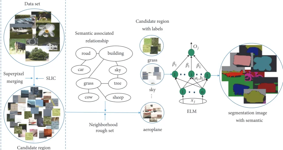
Figure 1: Flow chart of algorithm framework.
generated by superpixel as the basic processing unit to infer semantic label and then selects various classifier models to learn the inferred label. The main idea is that the superpixels or candidate regions with the same semantic label have similar appearance [7]. However, semantic label inference based on superpixel contains more redundant information, which can interfere with the accuracy. Although the methods based on candidate regions contain less redundant informa-tion, it is difficult to completely and accurately segment the number of image objects equaling the number of the labels by the current image segmentation techniques. Then the based multigraph model method uses all pixels or superpixels in the image as graph model nodes. And graph model is estab-lished with relationship between pixels or superpixels. But this method calculates a one-dimensional potential energy function for each superpixel and the algorithm complexity is high [8]. Fortunately, sparse representation and image hashing are powerful tools for data representation and the combinations of these two tools for scalable image retrieval. It is possible to replace the high-dimensional features with a low-dimensional Hamming space with preserving the similarity between features, which will reduce the computa-tional complexity of the energy function, thereby reducing the complexity of the algorithm [9–14]. In addition, the deep convolutional neural network based method uses a pretrained classification network to obtain objects of the image and then fine tunes by segmentation networks and image-level labels. The methods are sensitive to the accuracy and dataset of the pretrained classification network. And the classification network can only identify small and discernible regions, which is insufficient for the inference of large-scale image-level semantic labels [15].
Although the weakly supervised image semantic segmen-tation based on the image-level labels is proposed constantly, its segmentation accuracy has a large room for refinement compared with the fully supervised image semantic seg-mentation. The main obstacles and difficulties lie in how to accurately implement the semantic label inference, that is, the accurate mapping from the image-level labels to image pixel positions. In addition, as a dense pixel-level label prediction task, not all features are equally important and discriminative for learning classification models [16]. Therefore, how to construct an effective model to infer semantic labels is also meaningful for improving the accuracy of weakly supervised image semantic segmentation.
to generate different neighborhood particles and starts from the highest frequency semantic label to infer. Then the other candidate regions semantic labels are inferred based on the strongest associated relationship, which solves the problem of semantic label mapping difficultly.(3)An ELM training method is proposed. It uses candidate region with semantic labels to train ELM, which can reduce the introduction of negative sample pixels in the training data and improve accuracy of classification.
2. Related Work
As the simplest and most effective form of weak supervision, image-level labels are widely used in weakly supervised image semantic segmentation. It is difficult to correspond to image objects if only image-level labels data is used for training, since image-level labels cannot provide accurate information to describe boundaries and locations of objects due to inherent ambiguity of image-level labels. According to the different methods of semantic label inference, the paper divides the weakly supervised image segmentation algorithm into three categories: classifier, multigraph model, and deep convolutional neural network based methods.
The classifier based method uses image-level labels as supervised information and divides all pixels or superpixels in the image contained target label into positive samples and other negative samples without target label. Then classifier is trained directly and the best classifier is obtained by iteratively optimizing loss function. For example, Wei et al. [23] trained a multilabel classification network, where pictures are classified through the network, and finally matched the classification information with higher confi-dence to the original picture to obtain association between semantic labels and locations. However, this method directly introduces the pixel points of target image block as object regions into many negative sample pixels, such as pixels belonging to the background. Subsequently, Wei et al. [19, 22] proposed a simple to complex framework (STC) in 2017, which firstly trains an initial segmentation network using simple images and then predicts the labels of simple images using the network and uses these labels to enhance train-ing semantic segmentation network. Finally, the enhanced network is used to predict labels of more complex images and train a better semantic segmentation network. However, this method requires collecting a large number of simple pictures; otherwise it is difficult to train a higher performance initialization network and continue to improve, and it has many training samples and long training time. Zhang et al. [18] proposed to use the spatial sparse reconstruction method to obtain an effective SVM classifier, which trains classifier by training data with noise, and to use method of subspace reconstruction to denoising and find optimal SVM classi-fier by iterative optimization. The methods iterate between generating temporary segmentation masks and learning with interim supervision. These methods benefit from pixel-level supervision; but errors easily accumulate in iterations.
The multigraph model based method uses all pixels or superpixels in the image as graph model nodes. And graph model is established with relationship between pixels or
superpixels. Vezhnevets et al. [8] proposed a multi-instance learning (MIL) framework for weakly supervised images segmentation. The algorithm regards each superpixel as an instance; each image is represented as a series of instance sets. Only labels of instance set are known, so image seg-mentation is converted to instance label inference. But the algorithm lacks the labels between superpixel pairs. In order to solve this problem, Vezhnevets et al. [17] proposed a multi-image model (MIM) based on the graph model and built a common probability graph model on the training set and test set using conditional random fields for each superpixel. The one-dimensional potential energy function establishes a binary potential energy function between superpixel pairs and finally approximates parameters of conditional random field by method of graph division. However, this method calculates a one-dimensional potential energy function for each superpixel and the algorithm complexity is high. In order to enrich the description of superpixel features, Vezh-nevets et al. [24] further proposed a series of parameterized structured models in which potential energy pairs are formed by multichannel visual features, and weight of each channel is determined by minimizing to distinguish different superpixel labels of trained segmentation model. The above graph-based algorithm has improved segmentation performance in weakly supervised environment, but it is limited by the low descriptiveness of the unary or binary potential energy function.
The method of deep convolutional neural network is based on DCNN framework, which is trained to obtain the object position. Oquab et al. [25] applied DCNN framework to generate a single point to infer the location of the object, but this method cannot detect multiple objects of same class in an image. Pinheiro et al. [21] and Pathak et al. [20] added segmentation constraints to final cost function to optimize parameters of DCNN image-level labels. However, the two methods generate coarse prediction because the algorithms generally do not use low-level cues.
3. The Proposed Method
The paper proposes a weakly supervised image semantic segmentation framework based on candidate regions and ELM. The framework of the paper consists of two phases of learning and testing. Among them, there are three basic steps in the learning phase:(1)candidate region segmentation using superpixel; (2) candidate region semantic inference using semantic label association;(3)candidate regions clas-sification using ELM. In the testing phase, the paper first performs superpixel segmentation and merging on the test image and then predicts the semantic label of each pixel with the candidate region as the basic processing unit.
3.1. Segmentation of Candidate Regions Using Superpixels.
Input: Data set, image-level label number𝑙.
Output: Cluster center for each target superpixel𝐶 = {𝑐𝑖}𝑛𝑖=1, the number of target superpixels in the image𝑛.
Step 1. SLIC superpixel segmentation,𝑋 = [𝑥1, . . . , 𝑥𝑛]. Step 2. While𝑛 ≥ 3𝑙
(a) Extract visual features of each superpixel: LAB(3 dim), Gabor(65 dim), Sift(64 dim), Surf(64 dim);
(b) The adjacency relationship between superpixels is counted and stored in matrix𝐷;
(c) The superpixel similarity𝑆is calculated according to formula (1);
(d) Combine the most similar superpixel pairs with considering the adjacency;
(e) Calculate the mean of the merged superpixel clustering centers as a new clustering center;
(f) Update𝑛.
End
Step 3. Reclassify disconnected areas.
Algorithm 1: Superpixel merging process.
visual features are extracted to preserve the boundary infor-mation of each superpixel as much as possible during the merging process. Therefore the paper selects the colour, texture, sift, and surf features representing each superpixel. Specifically, due to the wide colour gamut of the LAB, this paper chooses the LAB as the colour feature. And this paper selects the Gabor filters to represent the texture feature of each superpixel, because the Gabor filter has the capability of dealing with spatial transformations [26].
First, the initial image is divided into superpixels based on the simple linear iterative clustering algorithm (SLIC). And compared with other superpixel segmentation methods, SLIC algorithm has the following advantages [27]: (a) the size of formed superpixels is basically the same; (b) the number of superpixels can be controlled by adjusting the parameterk; (c) the speed is fast and boundary fit between block and target boundary is high; d) the difference of features between pixels within each block is small.
Then, the 196-dimensional visual features are extracted to describe each superpixel, including colour features (3-dimension), texture features (65-(3-dimension), Sift features (64-dimension), and Surf features (64-dimension). Finally, on the basis of superpixel spatial position adjacency, the most similar superpixels are merged by statistical superpixel similarity, and the number of superpixels is combined to be no more than three times of image labels, as shown in Figure 2.
Suppose an image contains nsuperpixels𝑋 = [𝑥1, . . . ,
𝑥𝑛] ∈ 𝑅𝑚×𝑛, and any superpixel𝑥
𝑖has 196 dimensional visual
features to describe, image labels𝑦 = [𝑦1, 𝑦2, . . . , 𝑦𝑙], andlis the number of image semantic labels. Then similarity of any superpixels𝑥𝑖and𝑥𝑗is described as
𝑆𝑖,𝑗
= ∑𝑚
𝑖=1,𝑗=1, 𝑎𝑛𝑑 𝑖 ̸=𝑗
[𝛿1𝑑𝑖𝑗𝑙𝑎𝑏+ 𝛿2𝑑𝑡𝑒𝑥𝑖𝑗 + 𝛿3𝑑𝑠𝑖𝑓𝑡𝑖𝑗 + 𝛿4𝑑𝑠𝑢𝑟𝑓𝑖𝑗 ]
× 𝐷𝑖,𝑗
(1)
where𝛿is weight factor of adjusting distance and satisfies𝛿1+
𝛿2+⋅ ⋅ ⋅+𝛿4= 1;𝑑𝑙𝑎𝑏𝑖𝑗 ,𝑑𝑡𝑒𝑥𝑖𝑗 ,𝑑𝑠𝑖𝑓𝑡𝑖𝑗 ,𝑑𝑠𝑢𝑟𝑓𝑖𝑗 are the Euclidean distance
to represent the color, texture, Sift, and Surf distance of the
superpixels𝑖and𝑗;𝐷stores adjacency relationship between superpixels.
𝐷𝑖,𝑗={{
{
1, if ci is adjacent to cj
0, otherwise (2)
The specific steps of superpixel merging algorithm are as shown in Algorithm 1.
3.2. Candidate Region Semantic Inference Using Semantic
Label Association. The inference from image-level to
pixel-level semantic label is the key of the whole weakly supervised image semantic segmentation algorithm. In the process, the classification of candidate regions directly affects the seman-tic label inference results; it is necessary to extract rich visual features. Therefore the paper adopts CNN to extract features to ensure effective classification results. However, extracting multilayer visual features increases the data dimension; it will bring great difficulties to subsequent label clustering. The neighborhood classifier [28] has an important advantage in that it can get a subset of the features that are important for decision making through attribute reduction; that is, it can obtain discriminative features that are important for semantic label inference.
As for the candidate region as the basic processing unit, the paper regards the semantic label inference as the most similar neighborhood particle extraction problem; the uniqueness of the program is as follows: (1) The paper stars inferring the semantic label from the semantic label with the most images, as much as possible to ensure the accuracy of prediction of the semantic labels;(2)According to the image-level label number and the proportion of the images corresponding to the semantic label to be inferred, the number of candidate regions is included in each semantic label to be inferred;(3)The inference of each semantic label is based on semantic label association relationship, which reduces the interference of the noise. The detailed steps are as follows:
First, semantic labels can be represented as 𝐿 =
[𝑙1, 𝑙2, . . . , 𝑙𝑘]; kis the total number of semantic labels
Superpixel segmentation
original image Superpixel segmentation
image
Superpixel merging
[image:5.600.86.520.73.176.2]Candidate region
Figure 2: Flow chart of candidate region segmentation based on superpixel.
horsevoid mountainboat bodydog cat road chair bookbird sign flower bicyclecar face water aeroplanesky sheepcow tree grass building
ca
t
ca
r
sky dog
tr
ee
face
co
w
bi
rd
sign voi
d
boa
t
ro
ad
gra
ss
chai
r
bod
y
boo
k
ho
rs
e
wa
ter
she
ep
flo
w
er
bi
cy
cl
e
b
u
ildin
g
aer
o
p
la
n
e
mo
un
ta
in
0.2 0.4 0.6 0.8 1
Figure 3: Image semantic correlation intensity map.
[𝑁(𝑡), 𝑡 = 1, 2, . . . , 𝑘]. According to the relationship between
LandN, it can obtain a semantic label containing the most images in the data set. Then the number of candidate region set corresponding to the semantic labelican be expressed as
𝑅𝑖= 𝑛𝑁 (𝑖) , 𝑛 ∈ 𝑅+ (3)
where𝑛is a proportional parameter. It depends on the multi-ple of the number of image-level labels and the commulti-plexity of the training set image. Therefore, the proportion of the candidate region set corresponding to the semantic label𝑖in the entire candidate region library can be expressed as
𝐹𝑖= 𝑅 (𝑖)
∑𝑘
𝑡=1𝑅 (𝑡)
(4)
Therefore, this paper obtains the range of the proportion of candidate regions set. And the inference of the semantic label is transformed into finding the proportion of candidate region corresponding to the semantic label.
Second, given a set of semantic labels that need to be associated, the semantic association relationship between labels is obtained by calculating the semantic association strength. And the association relationship is saved in a diagonal relationship matrix𝑊expressed as
𝑊𝑘×𝑘={{
{
𝐿𝑖,𝑗, ( 𝑖 > 𝑗)
0, (𝑖 ≤ 𝑗) (5)
𝐿𝑖,𝑗= 𝑐𝑜𝑚𝑖,𝑗
𝑐𝑜𝑓𝑖,𝑗 (6)
where𝐿𝑖,𝑗is connection strength of two labels𝑖and𝑗in the data set,𝑐𝑜𝑚𝑖,𝑗 is frequency of simultaneous occurrence of labels𝑖and𝑗, and𝑐𝑜𝑓𝑖,𝑗is frequency of any one occurrence of labels 𝑖 and 𝑗. Semantic association strength is shown in Figure 3. The color from blue to red indicates that association strength is from weak to strong in the figure. And image semantic self-association is the strongest degree that is expressed as red.
As can be seen from Equation (4) and (5), this paper encourages inference from semantic labels that appear simul-taneously in multiple images. Then the sematic labels are inferred from the strongest association. According to the semantic label association relationship and its corresponding semantic label, the proportion of the semantic label can be obtained.
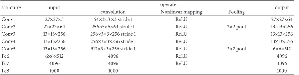
[image:5.600.136.466.214.421.2]Table 1: Network structure of CNN.
structure input operate output
convolution Nonlinear mapping Pooling
Conv1 27×27×3 64×3×3×3 stride 1 ReLU 27×27×64
Conv2 27×27×64 256×5×5×64 stride 1 ReLU 2×2 pool 13×13×256
Conv3 13×13×256 256×3×3×256 stride 1 ReLU 13×13×256
Conv4 13×13×256 256×3×3×256 stride 1 ReLU 13×13×256
Conv5 13×13×256 512×3×3×256 stride 1 ReLU 2×2 pool 6×6×512
Fc6 6×6×512 4096 ReLU 4096
Fc7 4096 4096 ReLU 4096
Fc8 1000 1000 1000
is shown in Table 1. It consists of five convolutional layers (cov1∼cov5) and three fully connected layers (fc6∼fc8). In this paper, five convolutional layers and two full convolutional layers are used for learning. After cov2 and cov5 convolution operations, the max pooling method is used to operate, and finally 4096-dimensional feature vector of fc7 layer is used as an image feature vector output. For CNN input data preparation phase, the sample patch uses an image block of 27×27 pixels in size, and the sampling center is candidate region center. For CNN output, feature extraction model chooses directly to use 4096-dimensional feature vector of fc7 layer as visual feature of candidate region.
According to the feature vector of the candidate region, we construct an information table𝐼𝑆 = ⟨𝑈, 𝐶, 𝑉, 𝑓⟩, where the sample set of candidate regions 𝑈 = {𝑥1, 𝑥2, . . . , 𝑥𝑘}, which is described by a series of features. Where𝑘 is the number of candidate regions in the candidate region library, 𝐶is feature set describing𝑈,𝑉is a set of attribute values, and 𝑓is information function. And the neighborhood particles 𝛿(𝑥𝑖)of each candidate region are constructed:
𝐹𝑥𝑖= 𝛿 ( 𝑥𝑈𝑖) (7)
𝛿 ( 𝑥𝑖) = {𝑥𝑗 | 𝑥𝑗∈ 𝑈, Δ (𝑥𝑖, 𝑥𝑗) ≤ 𝛿} (8)
Δ (𝑥𝑖, 𝑥𝑗) = (∑𝑚
𝑖=1𝑓(𝑥𝐼
, 𝐶) − 𝑓 ( 𝑥𝐽, 𝐶)𝑃)
1/𝑃
(9)
where𝛿 ≥ 0;𝛿(𝑥𝑖)is called generated neighborhood informa-tion particle, which determines the size of the neighborhood particle.𝑃is the norm,Δis called the similarity measure, and 𝑚is dimension of attribute matrix𝑉. According to nature of metric, it can be known that
𝛿 (𝑥𝑖) ̸= ⌀ (10)
𝑘
∑
𝑖=1
𝛿 ( 𝑥𝑖) = 𝑈 (11)
If the size of the neighborhood particle is fixed, the neigh-borhood particle with the most similar candidate regions can be obtained. And 𝑓𝑖 can determine the size of the neighborhood particle. Then the paper can get neighborhood thresholds𝛿 = {𝛿1, 𝛿2, . . . , 𝛿𝑘}and get the smallest threshold
𝛿V=min(𝛿). Therefore, the candidate regions corresponding to the most similar neighborhood particles with the mini-mum threshold are determined.
Finally, the paper obtains the candidate region corre-sponding to the semantic label to be inferred and its neigh-boring particles and completes the inference of the semantic label. After that, the inferred candidate region is removed from the candidate region library, iterating until all inferences of the rest of semantic labels are completed.
3.3. Candidate Regions Classification Using ELM. After
com-pleting the inference of all semantic labels, the paper selects the ELM to learn the inferred candidate regions. The main reason is that ELM is a new type of fast machine learning algorithm, which is a supervised algorithm based on single hidden layer feed forward neural network [29]. In addition, ELM trains parameters without iterating, which can improve algorithm efficiency.
First, the ELM is trained based on candidate regions with semantic labels and get trained ELM to classify in the training stage. And the candidate region is still used as the basic processing unit of semantic label prediction. The reason is that the candidate region is well close to the boundary of the target and is not susceptible to noise. In order to obtain the candidate regions corresponding to the test images, the paper first performs superpixel segmenta-tion and superpixel merging to generate candidate regions under the same parameter setting and implementation steps. Then 4096-dimensional features are extracted on the can-didate regions corresponding to the test images to ensure the consistency between the testing stage and the training stage.
After that, given an image candidate region 𝑥𝑖 =
{𝑥1, 𝑥2, . . . , 𝑥𝑙}in the ELM testing stage,𝑙is the number of
the test candidate regions. The candidate region is directly used as the input of the ELM; then the semantic label is predicted by the ELM. The specific steps of the ELM classification algorithm are shown in Algorithm 2.
4. Experiment
4.1. Dataset and Evaluation. The performance of our
Input: Given𝑁training samples(𝑥𝑖, 𝑦𝑖),𝑖 = 1, 2, . . . , 𝑁; The number of semantic label categories𝑘;
Activation function𝑔(𝑥); The number of hidden layer nodes is l𝑙, Test sample𝑥.
Output: Predicted result𝑦.
Step 1. Initialize the weight and bias between the input layer and the hidden layer, Randomly set
the value of𝑤and𝑏, given the value of𝑙.
Step 2. Select the activation function of the hidden layer𝑔(𝑥)and calculating the output matrix𝐻. Step 3. Calculate the output weight of the network𝛽:𝛽 = 𝐻𝑇𝑇(where𝐻𝑇is the transpose of𝐻). Step 4. The output weights of the test samples𝑥:𝑂𝑖= 𝐻(𝑤1, . . . , 𝑤𝑙, 𝑥, 𝑏1, . . . , 𝑏𝑙) ̂𝛽.
Step 5. the output of the predicted result𝑦:𝑦= 𝑙𝑎𝑏𝑒𝑙(𝑥) =arg max(𝑂𝑖), (1 ≤ 𝑖 ≤ 𝑘).
Algorithm 2: ELM classification algorithm.
structured scenes (such as buildings and roads), and other structures scenes. The dataset provides pixel-level annotation semantic images, and all images corresponding to pixel-level annotations maps are 213×320 pixels in size. And the scene contains a total of 23 semantic categories of objects. The same rules are followed in use of dataset, ignoring the classes of the horse and mountain image type. This article uses 276 images for training and 256 images for testing.
In addition, our method is also evaluated on the PASCAL VOC 2012 segmentation benchmark dataset [31], which is one of the most widely used benchmark datasets for semantic segmentation. It contains one background category and 20 object categories. It consists of three parts: training set (1464 images), validation set (1449 images), and test set (1456 images). In our experiments, our work is also based on the training images (10582 images) amplified by Harry Harlan et al. [32] as a training set, which provides image-level labels for training.
In this paper, evaluation index selects pixel accuracy (PA), mean pixel accuracy (MPA), and mean intersection over union (mIoU). Calculation formula is as follows:
𝑃𝐴 = ∑𝑖𝑛𝑖𝑖
∑𝑖𝑡𝑖 (12)
𝑀𝑃𝐴 = 1
𝑛𝑐𝑙∑𝑖
𝑛𝑖𝑖
𝑡𝑖 (13)
𝑚𝐼𝑜𝑈 = 1
𝑛𝑐𝑙∑𝑖
𝑛𝑖𝑖
(𝑡𝑖+ ∑𝑗𝑛𝑗𝑖− 𝑛𝑖𝑖) (14)
where𝑛𝑐𝑙is the number of categories included in true value, 𝑛𝑗𝑖is the pixel of category𝑖divided into category𝑗, and𝑡𝑖is the total number of pixels of category𝑖in ground truth.
4.2. Parameter Settings. The parameter setting of CNN model
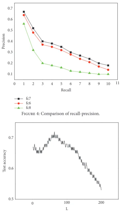
is given as follows. The learning rate was set to 0.001, and the performance of three CNN visual features in image clus-tering is analyzed and compared. The last 3 fully connected extracted visual characteristics of candidate regions, whose outputs are 4096, 4096, and 1000, respectively, are considered feature representations of image. Figure 4 shows comparison of three visual features on MSRC dataset. It can be seen that visual features are selected as output of fc7 layer for image clustering, whose precision is the highest.
The parameter setting of ELM algorithm is given as follows. When designing ELM, the cross-validation method
fc7 fc6 fc8
8
2 4 6 10
0 1 3 5 7 9 11
Recall
0.1 0.2 0.3 0.4 0.5 0.6 0.7
P
re
cisio
[image:7.600.312.543.225.629.2]n
Figure 4: Comparison of recall-precision.
0.5 0.6 0.7
T
es
t acc
urac
y
200
0 100
[image:7.600.106.290.475.552.2]L
Figure 5: Relationship between L and test accuracy.
Image Ground truth Prediction Image Ground truth Prediction
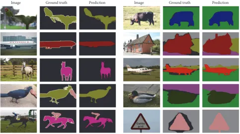
Figure 6: Examples of predicted segmentations (the left are the examples of MSRC and the right are the examples of PASCAL VOC 2012 dataset).
the measurement accuracy of ELM is generally decreasing. So when 60≤L≤68, ELM has a good test accuracy.
4.3. Experimental Results. In order to evaluate the
perfor-mance of the proposed weakly supervised image semantic segmentation method, the experiments were compared with the current weakly supervised image semantic segmentation algorithm on the MSRC-21 dataset and PASCAL VOC 2012 dataset. These comparison algorithms include STC [19], AE [22], SR [18], MIM [17], MIL+ILP+SP-sppxly [21], and CCNN [20], and these weakly supervised image semantic segmentation comparison algorithms are based on image-level labels.
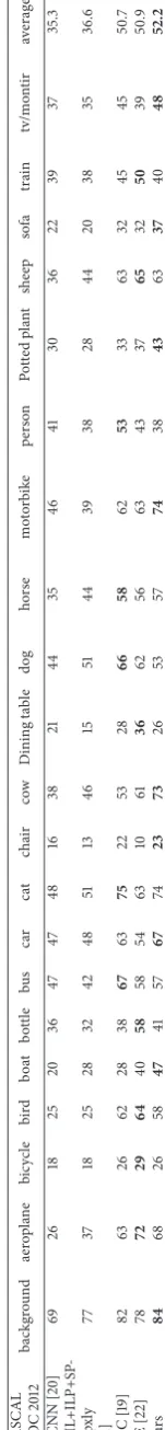
First, the IoU of per-image label and the average IoU (mIoU) of all image labels are as in Tables 2 and 3, respec-tively, for the proposed method and the current weakly supervised image semantic segmentation algorithm on the MSRC-21 dataset and the PASCAL VOC 2012 dataset. And each column represents different algorithm accuracy of each semantic class on MSRC-21 and PASCAL VOC 2012 dataset, and the last column is average accuracy of all classes. The bold values in the table represent the best segmentation performance.
As shown in Tables 2 and 3, the proposed algorithm obtains comparable and competitive results on the IoU of per-image label and the average IoU (mIoU) of all semantic labels compared with the existing image-level labels weakly supervised image semantic segmentation algorithm method. Although the IoU on some semantic classes is lower than the compared algorithm on the MSCR and the PASCAL VOC 2012 validation set, the proposed algorithm achieves
the best segmentation performance on the mIoU. In addition, the segmentation accuracy for the weakly supervised image semantic segmentation algorithm on the MSRC dataset is significantly higher than that of the PASCAL VOC 2012 dataset. The reason is that the images on the PASCAL VOC 2012 dataset contain more complex objects and backgrounds than the images on the MSRC dataset. Although many weakly supervised image semantic segmentation algorithms have been proposed, the segmentation accuracy of each semantic class on the entire dataset still has a relatively large room for improvement.
Then, in order to more intuitively display the segmenta-tion performance of the proposed algorithm, some qualitative segmentation examples of MSRC and PASCAL VOC 2012 dataset are given. The specific segmentation results are shown in Figure 6.
As shown in Figure 6, the weakly supervised deep seman-tic segmentation using CNN and ELM with semanseman-tic candi-date regions can achieve better segmentation performance. Moreover, the segmentation result based on the candidate region level can retain the edge information of the object in the image. However, the proposed method relies on semantic label inference and classifier learning at the candidate region level for an object that contains multiple regions with large contrast, which may be misclassified.
5. Conclusions
proposed. By merging superpixels into candidate regions instead of using a large number of superpixels in an image, the semantic associated relationship and neighborhood rough set are effectively combined to solve the difficulty of map-ping from semantic labels into image objects. The image semantic labels quantity information is used as a condition to terminate superpixel merging, which avoids problem of manually set parameters and hence helps to solve the problem of nonadjacent multiple instances. The candidate regions are classified based on neighborhood rough set, where the candidate regions are inferred by using semantic associated relationship. As a result, more reliable candidate region semantic labels can be obtained to improve the classification accuracy. Future works can be extended to combine saliency detection [33, 34] and heuristic optimization in a data fusion framework [35–38].
Data Availability
The data used to support the findings of this study are available from the corresponding author upon request.
Conflicts of Interest
The authors declare that there are no conflicts of interest regarding the publication of this paper.
Acknowledgments
The authors would like to express their gratitude for the support from the National Natural Science Foundation of China (61503271; 61603267), Shanxi Scholarship Council of China (2015-045; 2016-044), 100 People Talents Programme of Shanxi, Shanxi Natural Science Foundation of China (201801D121144), and Shanxi Natural Science Foundation of China (201801D221190).
References
[1] Z. Shi and Y. Yang, “Weakly-supervised image annotation and
segmentation with objects and attributes,”IEEE Transactions on
Pattern Analysis and Machine Intelligence, vol. 39, no. 12, pp. 2525–2538, 2017.
[2] J. Gao, Z. Xie, J. Zhang et al., “Image semantic analysis and
understanding: a review,” Pattern recognition and artificial
intelligence, vol. 2, no. 23, pp. 191–202, 2010.
[3] H. Noh, S. Hong, and B. Han, “Learning deconvolution network
for semantic segmentation,” inProceedings of the IEEE
Inter-national Conference on Computer Vision, ICCV 2015, pp. 1520– 1528, Santiago, Chile, December 2015.
[4] J. Long, E. Shelhamer, and T. Darrell, “Fully convolutional
networks for semantic segmentation,” inProceedings of the IEEE
Conference on Computer Vision and Pattern Recognition, CVPR
2015, pp. 3431–3440, Boston, Mass, USA, June 2015.
[5] G. Papandreou, L. Chen, K. P. Murphy et al., “Weakly-and semi-supervised learning of a deep convolutional network
for semantic image segmentation,” inProceedings of the IEEE
International Conference on Computer Vision (ICCV 2015), pp. 1742–1750, Santiago, Chile, December 2015.
[6] D. Lin, J. Dai, J. Jia et al., “Scribblesup: scribble-supervised
convolutional networks for semantic segmentation,” in
Proceed-ings of the IEEE Conference on Computer Vision and Pattern Recognition, CVPR 2016, pp. 3159–3167, Las Vegas, Nev, USA, July 2016.
[7] Z. Lu, Z. Fu, T. Xiang, P. Han, L. Wang, and X. Gao, “Learning
from weak and noisy labels for semantic segmentation,”IEEE
Transactions on Pattern Analysis and Machine Intelligence, vol. 39, no. 3, pp. 486–500, 2017.
[8] A. Vezhnevets and J. M. Buhmann, “Towards weakly supervised semantic segmentation by means of multiple instance and
multitask learning,” inProceedings of the 2010 IEEE Computer
Society Conference on Computer Vision and Pattern Recognition, CVPR 2010, pp. 3249–3256, San Francisco, Calif, USA, June 2010.
[9] Y. Xi, J. Zheng, X. Li, X. Xu, J. Ren, and G. Xie, “SR-POD: sample rotation based on principal-axis orientation distribution for
data augmentation in deep object detection,”Cognitive Systems
Research, vol. 52, pp. 144–154, 2018.
[10] Y. Yan, J. Ren, G. Sun et al., “Unsupervised image saliency detection with Gestalt-laws guided optimization and visual
attention based refinement,”Pattern Recognition, vol. 79, pp. 65–
78, 2018.
[11] G. Ding, J. Zhou, Y. Guo et al., “Large-scale image retrieval with
sparse embedded hashing,”Neurocomputing, vol. 257, pp. 24–36,
2017.
[12] G. Wu, J. Han, Z. Lin et al., “Joint image-text hashing for fast large-scale cross-media retrieval using self-supervised deep
learning,”IEEE Transactions on Industrial Electronics, pp. 1-1,
2018.
[13] G. Wu, J. Han, Y. Guo et al., “Unsupervised deep video
hashing via balanced code for large-scale video retrieval,”IEEE
Transactions on Image Processing, vol. 28, no. 4, pp. 1993–2007, 2019.
[14] Y. Guo, G. Ding, J. Han, and Y. Gao, “Zero-shot learning with
transferred samples,”IEEE Transactions on Image Processing,
vol. 26, no. 7, pp. 3277–3290, 2017.
[15] Y. Wei, H. Xiao, H. Shi et al., “Revisiting dilated convolution: a simple approach for weakly- and semi-supervised semantic
seg-mentation,” inProceedings of the IEEE Conference on Computer
Vision and Pattern Recognition. CVPR 2018, pp. 7268–7277, Salt Lake City, Utah, USA, June 2018.
[16] Y. Liu, J. Liu, Z. Li et al., “Weakly-supervised dual clustering for
image semantic segmentation,” inProceedings of the IEEE
Con-ference on Computer Vision and Pattern Recognition (CVPR), pp. 2075–2082, Portland, Ore, USA, June 2013.
[17] A. Vezhnevets, V. Ferrari, and J. M. Buhmann, “Weakly super-vised semantic segmentation with a multi-image model,” in Proceedings of the IEEE International Conference on Computer Vision, ICCV 2011, pp. 643–650, Barcelona, Spain, November 2011.
[18] K. Zhang, W. Zhang, Y. Zheng et al., “Sparse reconstruction
for weakly supervised semantic segmentation,” inProceedings of
the International Joint Conference on Artificial Intelligence, IJCAI
2013, pp. 1889–1895, Beijing, China, August 2013.
[19] Y. Wei, X. Liang, Y. Chen et al., “STC: a simple to com-plex framework for weakly-supervised semantic segmentation,” IEEE Transactions on Pattern Analysis and Machine Intelligence, vol. 39, no. 11, pp. 2314–2320, 2017.
in Proceedings of the 15th IEEE International Conference on Computer Vision, ICCV 2015, pp. 1796–1804, Chile, December 2015.
[21] P. O. Pinheiro and R. Collobert, “From image-level to
pixel-level labeling with convolutional networks,” inProceedings of the
IEEE Conference on Computer Vision and Pattern Recognition (CVPR), pp. 1713–1721, Boston, Mass, USA, June 2015. [22] Y. Wei, J. Feng, X. Liang, M.-M. Cheng, Y. Zhao, and S.
Yan, “Object region mining with adversarial erasing: a simple
classification to semantic segmentation approach,” in
Proceed-ings of the IEEE Conference on Computer Vision and Pattern Recognition, CVPR 2017, Hawaii, USA, July 2017.
[23] Y. Wei, X. Liang, Y. Chen et al., “Learning to segment with
image-level annotations,”Pattern Recognition, vol. 59, pp. 234–
244, 2016.
[24] A. Vezhnevets, V. Ferrari, and J. M. Buhmann, “Weakly super-vised structured output learning for semantic segmentation,” inProceedings of the IEEE Conference on Computer Vision and Pattern Recognition, CVPR 2012, pp. 845–852, Providence, RI, USA, June 2012.
[25] M. Oquab, L. Bottou, I. Laptev, and J. Sivic, “Learning and transferring mid-level image representations using
convolu-tional neural networks,” inProceedings of the IEEE Conference
on Computer Vision and Pattern Recognition (CVPR ’14), pp. 1717–1724, IEEE, Columbus, Ohio, USA, June 2014.
[26] S. Luan, C. Chen, B. Zhang, J. Han, and J. Liu, “Gabor
convo-lutional networks,”IEEE Transactions on Image Processing, vol.
27, no. 9, pp. 4357–4366, 2018.
[27] R. Achanta, A. Shaji, K. Smith, A. Lucchi, P. Fua, and S. S¨usstrunk, “SLIC superpixels compared to state-of-the-art
superpixel methods,”IEEE Transactions on Pattern Analysis and
Machine Intelligence, vol. 34, no. 11, pp. 2274–2281, 2012. [28] Q. Hu, “Numerical attribute reduction based on neighborhood
granulation and rough approximation,”Journal of Software, vol.
19, no. 3, pp. 640–649, 2008.
[29] G. B. Huang, Q. Y. Zhu, and C. K. Siew, “Extreme learning machine: a new learning scheme of feedforward neural
net-works,” inProceedings of the IEEE International Joint Conference,
vol. 2, pp. 985–990, Budapest, Hungary, March 2004.
[30] J. Shotton, J. Winn, C. Rother et al., “Textonboost: joint appearance, shape and context modeling for multi-class object
recognition and segmentation,” inProceedings of the European
Conference on Computer Vision, ECCV 2006, vol. 3951, Graz, Austria, May 2006.
[31] M. Everingham, L. van Gool, C. K. I. Williams, J. Winn, and A. Zisserman, “The pascal visual object classes (VOC) challenge,” International Journal of Computer Vision, vol. 88, no. 2, pp. 303– 338, 2010.
[32] B. Hariharan, P. Arbel´aez, L. Bourdev, S. Maji, and J. Malik,
“Semantic contours from inverse detectors,” inProceedings of
the IEEE International Conference on Computer Vision, ICCV
2011, pp. 991–998, Barcelona, Spain, November 2011.
[33] Z. Wang, J. Ren, D. Zhang, M. Sun, and J. Jiang, “A deep-learning based feature hybrid framework for spatiotemporal saliency
detection inside videos,”Neurocomputing, vol. 287, pp. 68–83,
2018.
[34] J. Han, D. Zhang, X. Hu, L. Guo, J. Ren, and F. Wu, “Background prior based salient object detection via deep reconstruction
residual,”IEEE Transactions on Circuits and Systems for Video
Technology, vol. 25, no. 8, pp. 1309–1321, 2015.
[35] Y. Yan, J. Ren, H. Zhao et al., “Cognitive fusion of thermal and visible imagery for effective detection and tracking of
pedestrians in videos,”Cognitive Computation, vol. 10, no. 1, pp.
94–104, 2018.
[36] A. Zhang, G. Sun, J. Ren et al., “A dynamic neighborhood
learning-based gravitational search algorithm,”IEEE
Transac-tions on Cybernetics, vol. 48, no. 1, pp. 436–447, 2018.
[37] J. Tschannerl, J. Ren, P. Yuen et al., “MIMR-DGSA: unsu-pervised hyperspectral band selection based on information theory and a modified discrete gravitational search algorithm,” Information Fusion, vol. 51, pp. 189–200, 2019.
[38] F. Cao, Z. Yang, and J. Ren, “Local block multilayer sparse extreme learning machine for effective feature extraction and
classification of hyperspectral images,”IEEE Trans. Geoscience
Hindawi
www.hindawi.com Volume 2018
Mathematics
Journal ofHindawi
www.hindawi.com Volume 2018
Mathematical Problems in Engineering Applied Mathematics Hindawi
www.hindawi.com Volume 2018
Probability and Statistics Hindawi
www.hindawi.com Volume 2018
Hindawi
www.hindawi.com Volume 2018
Mathematical PhysicsAdvances in
Complex Analysis
Journal ofHindawi
www.hindawi.com Volume 2018
Optimization
Journal ofHindawi
www.hindawi.com Volume 2018
Hindawi
www.hindawi.com Volume 2018 Engineering Mathematics International Journal of
Hindawi
www.hindawi.com Volume 2018
Operations Research
Journal of
Hindawi
www.hindawi.com Volume 2018
Function Spaces
Abstract and Applied Analysis Hindawiwww.hindawi.com Volume 2018
International Journal of Mathematics and Mathematical Sciences
Hindawi
www.hindawi.com Volume 2018
Hindawi Publishing Corporation
http://www.hindawi.com Volume 2013
Hindawi www.hindawi.com
World Journal
Volume 2018Hindawi
www.hindawi.com Volume 2018Volume 2018
Numerical Analysis
Numerical Analysis
Numerical Analysis
Numerical Analysis
Numerical Analysis
Numerical Analysis
Numerical Analysis
Numerical Analysis
Numerical Analysis
Numerical Analysis
Numerical Analysis
Numerical Analysis
Advances inAdvances in Discrete Dynamics in Nature and Society Hindawiwww.hindawi.com Volume 2018
Hindawi www.hindawi.com
Differential Equations International Journal of
Volume 2018
Hindawi
www.hindawi.com Volume 2018
Decision Sciences
Hindawi
www.hindawi.com Volume 2018
Analysis
International Journal of
Hindawi
www.hindawi.com Volume 2018