Accurate and efficient computation of the Boltzmann equation for Couette flow : influence of intermolecular potentials on Knudsen layer function and viscous slip coefficient

Contents lists available atScienceDirect

Journal

of

Computational

Physics

www.elsevier.com/locate/jcp

Accurate

and

efficient

computation

of

the

Boltzmann

equation

for

Couette

flow:

Influence

of

intermolecular

potentials

on

Knudsen

layer

function

and

viscous

slip

coefficient

Wei Su

a

,

1

,

Peng Wang

a

,

1

,

Haihu Liu

b

,

Lei Wu

a

,

∗

a_{James Weir Fluids Laboratory, Department of Mechanical and Aerospace Engineering, University of Strathclyde, Glasgow G1 1XJ, UK} b_{School of Energy and Power Engineering, Xi’an Jiaotong University, 28 West Xianning Road, Xi’an 710049, China}

a

r

t

i

c

l

e

i

n

f

o

a

b

s

t

r

a

c

t

Article history: Received6August2018

Receivedinrevisedform8November2018 Accepted9November2018

Availableonline13November2018

Keywords: Kramer’sproblem Boltzmannequation Gas-kinetictheory Knudsenlayer Viscousslipcoefficient Syntheticiterationscheme

The Couette flow is one ofthe fundamental problemsof rarefiedgas dynamics, which has been investigated extensivelybased on the linearized Boltzmann equation(LBE) of hard-spheremoleculesandsimplifiedkineticmodelequations.However,howthedifferent intermolecular potentialsaffecttheviscous slipcoefficientand thestructure ofKnudsen layerremainsunclear.Here,a novelsyntheticiterationscheme(SIS)isdevelopedforthe LBEto findsolutions ofCouetteflowaccuratelyand efficiently:the velocitydistribution functionisfirstsolvedbytheconventionaliterativescheme,thenitismodifiedsuchthat ineachiterationi) theflowvelocityisguidedbyanordinarydifferentialequationthatis asymptotic-preservingattheNavier–Stokes limitand ii) theshearstressis equaltothe averageshearstress.BasedontheBhatnagar–Gross–Krookmodel,theSISisassessedtobe efficientandaccurate.ThenweinvestigatetheKnudsenlayerfunctionforgasesinteracting throughthe inversepower-law,shielded Coulomb,and Lennard-Jones potentials,subject to diffuse-specular and Cercignani–Lampis gas-surface boundary conditions. When the tangential momentum accommodation coefficient (TMAC) is not larger than one, the Knudsen layer functionisstrongly affectedby the potential,where itsvalue and width increasewiththeeffectiveviscosityindexofgasmolecules.Moreover,theKnudsenlayer function exhibits similarities among different values of TMAC when the intermolecular potential is fixed. For Cercignani–Lampis boundary condition with TMAC larger than one, both the viscous slip coefficient and Knudsen layer function are affected by the intermolecular potential, especiallywhenthe “backward” scatteringlimitis approached. WiththeasymptotictheorybyJiangandLuo(2016)[14] forthesingularbehaviorofthe velocitygradient inthevicinity ofsolidsurfaces,wefindthatthe wholeKnudsenlayer functioncanbewellfittedbythepowerseries2n=0

2

m=0cn,mxn(xlnx)m,wherexisthe

distancetothesolidsurface.Finally,theexperimentaldataoftheKnudsenlayerprofileare explainedbytheLBEsolutionwithpropervaluesoftheviscosityindexandTMAC. ©2018TheAuthors.PublishedbyElsevierInc.ThisisanopenaccessarticleundertheCC

BYlicense(http://creativecommons.org/licenses/by/4.0/).

*

Correspondingauthor.

E-mail address:[email protected](L. Wu).

1 _{Bothauthorscontributedequally.}

https://doi.org/10.1016/j.jcp.2018.11.015

[image:2.561.183.371.57.178.2]

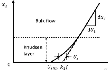
Fig. 1.SchematicdiagramoftheKnudsenlayerintheKramer’sproblem.Thevelocitydefect(Knudsenlayerfunction)

U

sdescribesthedeviationofthe linearlyextrapolatedvelocity(dashline)inthebulkregionfromthetruevelocity(solidline).Thevelocityslopeinthebulkregionis(dU1/dx2)|x2→∞=k1,

thesliplengthisζ,whiletheviscousslipcoefficientisdefinedasζ¯=ζ /λe,whereλeistheequivalentmeanfreepathofgasmolecules.

1. Introduction

TheKramer’sproblemdescribinggasflowoveraplanedrivenbyviscousstressisfundamentaltosolutionsofalmostall momentum transferproblemsofrarefiedgasdynamics [1]. AsillustratedinFig.1,whenthe planarwallat x2

=

0 moves slowlyinthehorizontaldirection,a nonlinearvelocityprofileandafiniteslipvelocitydevelopnearthesurface.Thiskinetic boundary layer,asknownastheKnudsenlayer,hasathicknessofseveralmeanfreepath

λ

ofgasmolecules.Due tothe infrequentgas–gasinteractions,theflowisessentiallyrarefied,sothattheconventionalNavier–Stokesequationsonlywork in the bulkregion butbreak down inthe Knudsenlayer. The linearizedBoltzmann equation (LBE)can be usedto study thisproblem.Forengineeringapplications,however,Navier–StokesequationsarestillpreferredwhentheKnudsennumber K n(the ratioof

λ

tothedimensionofflowdomain)issmall, duetoitsdistinctcomputational advantageovertheLBEin six-dimensionalphasespace.

Many effortshavebeenmadeto predictthe rarefiedgasflow, through incorporatingtherarefaction effectscausedby the presence ofsolid surface into hydrodynamic equations [2].For isothermal flows atsmall K n, itis adequate toapply thevelocity slipboundarycondition (BC)totheNavier–Stokesequations.Inthiscase,theviscousslipcoefficient(

ζ

¯

,VSC), as defined in Fig.1, is needed. The first estimation

ζ (

¯

α

)

=

(

2

−

α

)/

α

is proposed by Maxwell using insightful physical arguments [3].Here,

α

isthetangentialmomentumaccommodationcoefficient(TMAC)describingthefractionofdiffusely reflectedmoleculesatthesolidsurface,whiletherestofmoleculesarereflectedspecularly.Almostonehundredyearslater, usingavariationalapproachfortheLBEanddiffuse-speculargas-surfaceBC,LoyalkaobtainedtheVSCwhichisgeneralized intothefollowingform [4,5]:

¯

ζ (

α

)

=

2

−

α

α

_¯

ζ (

1

)

−

0

.

1211

(

1

−

α

)

.

(1)

Subsequently,lotsofinvestigationswerecarriedouttocalculatetheVSC bynumericallysolvingtheLBEanditssimplified model equations.It isfound that VSCsfromthe LBEandits kinetic model equationshavea relative difference lessthan 3% when the effectiveTMACis fixed [5]. It should be notedthat, althoughthe influence ofintermolecularpotentials on VSC hasbeenassessed by Loyalka usingthe variationalresults [6] and by Sharipov comparing theresults fromdifferent literatures [7], a systematic investigation of the role of intermolecularpotential on the VSC under different gas-surface interactionsonthebasisofthehighlyaccurateBoltzmannsolutionsisstillabsent.

When K nbecomes appreciable,the Navier–Stokesequations maybestill used, butinadditionto thevelocity slipBC the effectiveviscosity mustbe modified to a function ofthe distanceto solid surfaces.Inthis case, thestructure ofthe Knudsenlayerprovidesacriticalinformationtoformulatetheeffectiveviscosity.Lockerbyet al. firstproposedacurve-fitted approximationtotheKnudsenlayerfunction(KLF)as [8]

Us

(

x

)

≈

7

20

(

1

+

x

)

2

,

(2)

wherexisthedistancetothesolidsurfacenormalizedbythemeanfreepath

λ

.AlthoughtheKLFisfittedfroma temper-aturejumpprobleminsteadoftheshearproblem, itisfoundthat theNavier–Stokesequationswiththeeffectiveviscosity can predict the velocity profiles inPoiseuille andCouette flows, up to K n

=

0

.

4. Later,by fittingthe data fromthe LBE solutionofhard-sphere(HS)gasandthedirectsimulationMonteCarlomethodforCouetteflow [9],Lilley & Saderobtained apower-lawKLF [10,11]:

whereC isaconstant andtheexponentn

≈

0

.

82.Despitethefactthat thefittingiscarriedoutintheregion 0

.

1

x

1, theypredictedthepower-lawdivergenceofthevelocitygradientinthevicinityofthesolidsurface,thatis,dUs

/

dx

→ ∞

as x

→

0.

The singular behavior ofvelocity gradientatthe planar surface isrigorouslyproved by Takata& Funagane, when an-alyzing the thermaltranspirationbasedon theLBE ofHS molecules [12].However, instead ofthepower-law divergence, they found thelogarithmic divergenceofthe velocitygradient; that is,thespatial singularity isnot strongerthan lnx in thevicinity ofthesolidsurface. Thisconclusionisconfirmedby Jiang& Luowho,throughthe asymptoticanalysisofthe Bhatnagar–Gross–Krook(BGK)gaskinetic model [13],foundthatthevelocityprofileofCouette flownearthesolidsurface canbedescribedbythefollowingpowerseries [14]:

Us(x

)

=

N

n=0 M

m=0

cn,mxn

(

xlnx

)

m

,

x

→

0

.

(4)

Itshouldbe notedthat mostcontributions totheKramer’sproblemfocused mainlyonthediffuse-specularBCandHS molecules(orsimplifiedkineticmodels).Howintermolecularpotentials(suchastheinversepower-law,shieldedCoulomb, andLennard-Jonespotentials)andothergas-kineticBCsaffecttheVSCandKLFremainsunclear.Thispaperisdedicatedto addressingthesequestionsthroughthenumericalsimulationoftheLBEforCouetteflowbetweentwoparallelplates,which canbetakenasaspecificexampletoinvestigatethebehaviorofKnudsenlayer.Weemphasisthat,however,thenumerical method to finding the KLF at small values of K n is not easy. For instance, the results provided by Takata & Funagane are limitedto K n

0

.

6,since the computational cost tofind the steady-statesolution ofthe kinetic equations becomes extremelylargeforsmallKnudsennumbers [12];however,thisrelativelargevalueofK nisunfortunatelynotsmallenough toavoidtheinterferencebetweenKnudsenlayers.Inthepresentpaper,wefirstdevelop anefficientandaccuratemethod tosolvetheLBEforCouetteflow,andtheninvestigatetheroleofintermolecularpotentialsandgas-surfaceBCsontheVSC andKLF.

Theremainderofthepaperisorganizedasfollows.In§2,theLBEforthesteadyCouetteflowofamonatomicgasand variouskineticBCsareintroduced.In§3,a syntheticiterationschemeisdevelopedtoboosttheconvergenceinfindingthe steady-statesolutionoftheCouetteflowinthenear-continuumregime. In§ 4,influencesofintermolecularpotentialsand gas-kineticBCsontheVSCandKLFaswellasthesingularityofvelocitygradientnearthesolidsurfaceandthesimilarityof theKLFareinvestigated.In§5,experimentalresultsgivenbyReynoldset al. [15] areproperlyexplained.Thepapercloses withsomefinialcommentsin§6.

2. ThelinearizedBoltzmannequation

ConsiderthesteadyCouetteflowofamonatomicgasbetweentwoinfiniteparallelplateslocatedatx2

=

0 andx2

=

H. Thetop platemovesalongthe x1 directionwitha velocity Vw,whilethebottomplatemoveswiththeopposite velocity.

Both plates are maintained at a fixed temperature Tw. This Couette flow can be used to study the Kramer’s problem,

providedthat thedistancebetweenthetwo platesislarge enoughsothat thereisno interferencebetweentheKnudsen layersnearthetwoplates [7].

Forsimplicity,weusedimensionlessvariablesunlessspecified.Thecoordinatex2isnormalizedbythedistancebetween thetwoplates H,themolecularvelocityvisnormalizedbythemostprobablespeed vm

=

2kBTw

/

m,andvelocity

distri-butionfunctions feq andharenormalizedbyn0/vm3,wheren0istheaveragenumberdensityofthegasmoleculesbetween theparallelplates,kB istheBoltzmannconstant,andmisthemassofgasmolecules.

When Vw is farsmallerthan themostprobablespeed vm,the velocitydistribution functionof gasmoleculescan be

linearizedaroundtheglobalequilibriumdistributionfunction feq

(

v

)

=

π

−3/2exp

(

−|

v

|

2

)

as:

f

(

x2

,

v

)

=

feq(v

)

+

Vw

vm

h

(

x2

,

v

),

(5)

where v

=

(

v1,v2,v3) isthe molecular velocity andh

(

x2,v

)

Vw

/

vm isthe smallperturbance (h is not necessarysmaller

comparedto feq).TheLBEforh

(

x2,v

)

is:

v2

∂

h

∂

x2

=

L

(

h

,

feq), (6)

wherethelinearizedBoltzmanncollisionoperatoris [16]:

L

=

B

(

|

u

|

, θ )

[

feq(v

)

h

(

v_∗

)

+

feq(v_∗

)

h

(

v

)

−

feq(v

)

h

(

v_∗

)

]

d

dv_∗

L+

−

ν

eq(v

)

h

(

v

),

(7)

ν

eq(v

)

=

B

(

|

u

|

, θ )

feq(v_∗

)

d

dv_∗

.

(8)

Notethat therelative velocityofthetwo moleculesbeforebinary collisionisu

=

v

−

v_∗,and

isaunitvector alongthe relativepost-collisionvelocityv

−

v_∗.Thedeflectionangle

θ

betweenthepre- andpost-collisionrelativevelocitiessatisfies cos

θ

=

·

u

/

|

u

|

,0

≤

θ

≤

π

.Finally, B

(

|

u

|

,

θ )

= |

u

|

σ

isthecollisionkernel,with

σ

beingthedifferentialcross-sectionthat isdeterminedbytheintermolecularpotential.

Inthepresentpaper,weconsidertheinversepower-lawpotentials,wherethecollisionkernelsaremodeledas [17,16]

B

(

|

u

|

, θ )

=

|

u

|

2(1−ω)

K sin

1 2−ω

θ

2

cos12−ω

θ

2

,

(9)

with

ω

beingtheviscosityindex(i.e.the shearviscosity

μ

ofthegasisproportional to Tω) and K anormalization con-stant [16]. HS and Maxwell molecules have

ω

=

0

.

5 and 1, respectively. Note that this type of collision kernel cannot describethechargedmoleculesinteractingthroughtheCoulombpotentialwith

ω

=

2

.

5.AsdiscussedintheChapter 10of Ref. [18],inreality,however,chargedmoleculesinteractthroughthefollowingshieldedCoulombpotential:

U

(

ρ

)

=

λd

ρ

exp

−

ρ

λd

,

(10)

where isrelatedtothestrengthofthepotential,

ρ

istheintermoleculardistance,and

λ

d istheDebyeshieldinglength.

Forsimplicity,weonlyconsiderthesingle-specieschargedmoleculesinteractingthroughtherepulsiveforce.Wealso con-sidernoblegasesinteractingthroughthefollowingLennard-Jonespotentials:

U

(

ρ

)

=

4

_d

ρ

12

−

d

ρ

6

,

(11)

wheredisthedistanceatwhichthepotentialiszero.ThedetailsofimplementationoftheLennard-Jonespotentialsinfast spectralmethodcanbefoundinRef. [19].

The differentialcross-sectionfortheaboveshieldedCoulomb andLennard-Jonespotentialscanbecalculatedaccording toSharipov&Bertoldo [20].ThenthelinearizedBoltzmanncollisionoperator (7) canbesolvedbythefastspectralmethod developedbytheauthors [19].

To fullydetermine the gasdynamics inspatially-inhomogeneous problems,the gas-surface BC is needed. The general form oftheBC, whichspecifiesthe relationbetweenthevelocity distributionfunction f

(

v

)

ofthereflected andincident gasmoleculesatsolidsurface,isgivenbelow:

vnf

(

v

)

=

vn<0

|

v_n

|

R

(

v

→

v

)

f

(

v

)

dv

,

vn

>

0

,

(12)

wherevandvarevelocitiesoftheincidentandreflectedmolecules,respectively,vn isthenormalcomponentofmolecular

velocityvdirectedintothegas,andR

(

v

→

v

)

isthenon-negativescatteringkernel.

Themostpopulargas-surfaceBCisthediffuse-specularone,withthescatteringkernelreading:

RM(v

→

v

)

=

α

M

m2vn

2

π

(

kTw)2exp

−

mv2

2kTw

+

(

1

−

α

M) δ

v

−

v

+

2nvn

,

(13)

where the constant

αM

isthe TMAC, witha value inthe rangeof 0

≤

αM

≤

1,and

δ

is the Diracdeltafunction. Purely diffusereflectionhas

αM

=

1.TheBCproposedbyCercignani&Lampishasalsobeenwidelyused,whichreads [21]:

RC L

v

→

v

=

m

2_v n

2

π α

n

α

t

(

2

−

α

t

) (

kTw)2

I0

√

1

−

α

nmvnvn

α

nkTw

×

exp

−

m

v2

n

+

(

1

−

α

n)vn

2

2kTw

α

n

−

m

vt

−

(

1

−

α

t

)

vt

2

2kTw

α

t(2

−

α

t

)

,

(14)

wherevt isthetangential velocity, I0(x

)

=

2π

0 exp

(

xcos

φ)

d

φ/

2

π

,and

αn

∈ [

0

,

1

]

and

αt

∈ [

0

,

2

]

aretheenergyand mo-mentum accommodationcoefficients,respectively. When

αn

=

αt

=

1 or

αn

=

αt

=

0,thefullydiffuseorspecular BCsare recovered,respectively,whilefor

αn

=

0 and

αt

=

2,theCercignani–Lampisscatteringkerneldescries“backward”scattering. Other typesofBCshavealsobeenproposedanddiscussed [22],butfortheKramer’sproblem,aswillbeshownbelow,the twoBCsareadequatetoexplaintheexperimentaldata [15].

U1

=

v1hdv

,

P12

=

2v1v2hdv

.

(15)

3. Numericalmethod:thesyntheticiterationscheme

Toresolve the singular behaviorof velocity gradientthat occursin thevicinity of thesolid surface [12,14], high spa-tialresolutionis required.This meansthat itisbetter tosolvekinetic equationsby time-implicitdeterministic numerical method,otherwisetherestrictionontheCourant–Friedrichs–Lewyconditionwillrenderthetimestepextremelysmalland hencethecomputational costenormous;also,thedirectsimulationMonteCarlomethodwillbe expensivetoresolvethe velocityprofileinverysmallcellsnearthesolidsurface;forexample,thesimulationsarelimitedtorelativelargeKnudsen numberswithlargecellsize [10,11].

ToavoidtheinterferenceofthetwoKnudsenlayers,themeanfreepathofgasmoleculesshouldbesufficientlysmaller thanthedistancebetweentwoparallelplates;orequivalently,therarefactionparameter

δ

=

H

λe

, λe

=

μ

(

Tw)vm

n0kBTw

,

(16)

should be sufficiently large. Here the equivalent mean free path

λ

e

=

(

2

/

√

π

)λ

, where

λ

is the mean free path of gas

molecules.Therefore,theKnudsennumberisK n

=

√

π

/

2

δ

.

Theintegro-differentialsystem (6) is usuallysolvedbytheconventionaliteration scheme.Giventhevalueofh(k)

₍

_x2,v

₎

atthek-thiterationstep,thevelocity distributionfunctionatthenextiterationstepiscalculatedbysolvingthefollowing equation [9,17,19]:

ν

eqh(k+1)

+

v2

∂

h(k+1)

∂

x2

=

L+

(

h(k)

,

feq), (17)

wherethederivativewithrespecttox2isusuallyapproximatedbyasecond-orderupwindfinitedifference,andthecollision operatorinEq. (7) can becalculatedbythefastspectralmethod [16,19] basedonthevelocitydistributionfunctionatthe k-thiterationstep.Theprocessisrepeateduntilrelativedifferencesbetweensuccessiveestimatesofmacroscopicquantities arelessthanaconvergencecriterion .

The conventional iteration scheme is efficientfor highly rarefied gas flows (when

δ

is very small), where converged solutions canbe quicklyfound afterseveral iterations.However, the numberofiteration increasessignificantly when K n decreases(or

δ

increases),especiallywhenthegasflowisinthenear-continuumregime [23,24].Thesebehaviorsareinfact aresultofthecompetitionbetweenthemolecularcollisionandstreaming.Inthefree-molecularflowregime,gasmolecules moveinstraightway(exceptthecollisionwithsolidsurfaces)sothat anydisturbanceatonepointcanbe quicklyfelt by allother spatial points,sotheexchange of“information” andhencetheconvergenceisfast.However,fornear-continuum flows, binary collisions dominate so that the exchange of information through streaming becomes very inefficient: the perturbancedecaysrapidlyduetofrequentbinarycollisions andtakesalongtime tobefeltby otherpoints.The implicit unifiedgas-kineticschememaybeusedtoachievefastconvergence [25],however,currentlythereisnoversion developed fortheLBE.

Tohaveaconvergence-acceleratedschemefortheLBE,syntheticequationsfortheevolutionofmacroscopicflow vari-ables that are asymptotic preserving the Navier–Stokes limit provides an alternative way to enhance the information exchange across the whole computational domain [24]. For the Navier–Stokes equationswhich can be derived fromthe BoltzmannequationthroughtheChapman–Enskogexpansiontothefirst-orderoftheKnudsennumber,thegoverning equa-tionforflowvelocityis

∂

U1

∂

x2

= −

δ

P12

,

(18)

whereP12isaconstantacrossthewholedomain.FortheLBE,theshearstressremainsaconstant(thiscanbeeasilyproven bymultiplying Eq. (6) with v1 andthenintegratingwithrespecttov),buttheequationforU1 containshigh-orderterms beyondtheNavier–Stokeslevel.Thatis,thegoverningequationisingeneralcanbeexpressedas

∂

U1

∂

x2

= −

δ

P12

+

High-order terms

.

(19)

Toobtainthesyntheticequation (19) thatwillfacilitatethefastconvergencetothesteady-state,wefirstrewriteEq. (7) asL

=

(

L

−

LBG K

)

+

LBG K,where

isthelinearizedcollisionoperatoroftheBGKequationforCouetteflowbetweentwoparallelplates [24].Thenmultiplying Eq. (6) by2v1v2 andintegratingtheresultingequationwithrespecttothemolecularvelocityv,weobtain

∂

U1

∂

x2

= −

δ

P12

+

2v1v2

(

L

−

LBG K

)

dv

−

∂

∂

x2

(

2v2₂

−

1

)

v1hdv

High-order terms

.

(21)

Itisobviousthat,inthenear-continuumregime where

δ

→ ∞

,thehigh-order termsintheright-handsideofEq. (21) are negligible comparedto

δ

P12,so thatthe derived syntheticequation isasymptoticpreserving theNavier–Stokes limit. With this macroscopic equation to update the flow velocity, we devise the following new iteration scheme to find the steady-statesolutionoftheLBE (6) quickly:

•

Duetothesymmetryconditionh

(

x2,v1,v2,v3)

= −

h

(

1

−

x2,v1,

−

v2,v3),thecomputationaldomainwillbelimitedto 0

≤

x2

≤

1

/

2.Whenh(k) andU₁(k) areknownatthek-thiteration,wecalculateoneofthehigh-orderterms H1

(

x2

)

=

2v1v2(L

−

LBG K

)

dv.Wealsocalculatethevelocitydistributionfunctionh(k+1/2)accordingtotheconventionaliteration

scheme (17),thatis,wesolvethefollowingequation:

ν

eqh(k+1/2)

+

v2

∂

h(k+1/2)

∂

x2

=

L+

(

h(k)

,

feq), (22)

byasecond-orderupwindfinitedifferenceinthebulkandafirst-orderupwindschemeatthesolidsurface [9].

•

Fromh(k+1/2)_{,wecalculatetheflowvelocityU}(k+1/2)

1

(

x2),theshearstress P (k+1/2)

12

(

x2),andoneofthehigh-orderterms H2(x2)

=

(

2v2₂

−

1

)

v1f dv.Wealsocalculatetheaverageshearstressas

¯

P

=

2

1/2

0

P₁₂(k+1/2)dx2

.

(23)

•

WeobtaintheflowvelocityU(₁k+1)bysolvingEq. (21) withthesecond-orderupwindfinitedifference,startingfromthe symmetricalboundaryconditionU1(x2

=

1

/

2

)

=

0,whereP12isreplacedby P

¯

.Thatis,

∂

U(₁k+1)

(

x2

)

∂

x2

= −

δ

P

¯

+

H1

(

x2

)

−

∂

H2

(

x2

)

x2

.

(24)

•

The velocity distribution functionh

(

x2,v

)

ismodified to incorporatethe changeof macroscopicflow velocity. Mean-while,theshearstressisadjustedtoitsmeanvalue P

¯

,forallspatialpoints.Thatis,

h(k+1)

=

h(k+1/2)

+

2

U₁(k+1)

−

U₁(k+1/2)

v1feq

+

2

¯

P

−

P₁₂(k+1/2)

v1v2feq. (25)

•

Theabovestepsarerepeateduntilconvergence.

Sincethegaskineticequationissolvedtogetherwiththemacroscopicequation (24) forflowvelocity,theabovescheme iscalledthesyntheticiterativescheme(SIS).NotethatalthoughtheSIShasbeenwidelyappliedtotheradiationtransport processes [26] and rarefied gas flows driven by local pressure, temperature, and concentration gradients [23,27–30] to overcome theslow convergenceinthe near-continuum flow regime,it isthe first time thatthe SIS isdeveloped forthe linearizedCouetteflow.

3.1. Numericaltestsofefficiencyandaccuracy

Numerical simulations are carried out to assess the efficiency and accuracy of the SIS. We consider the simple BGK kineticmodelwiththediffuseboundaryconditionasithasrecentlybeensolvedwithhighaccuracy [14,31,32].

WefirsttesttheefficiencyoftheSIS.Wechoosetherarefactionparameter

δ

=

100 anddiscretizethehalfspatialspace into 50even-spacedpoints. Themolecular velocityspace v1 andv3 arediscretizedby therootsofthephysicists’version ofthefourth-order Hermitepolynomial, whilethemolecularvelocity v2 istruncatedto

[−

6

,

6

]

andapproximatedby the non-uniformpoints [16,33]:

v2

=

6

(

Nv

−

1

)

ı

[

(

−

Nv

+

1

)

ı

, (

−

Nv

+

3

)

ı

,

· · ·

, (

Nv

−

1

)

ı

]

,

(26)

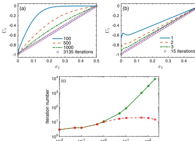
[image:7.561.100.441.51.296.2]

Fig. 2.Profilesoftheflowvelocityatdifferentiterationstepsobtainedfromtheconventionaliterationscheme (a)andSIS (b),whenδ=100.Circlesshow theconvergedsolution.(c) Thetotaliterationnumberneededtoobtaintheconvergedsolutionasafunctionoftherarefactionparameterδ,wherecircles andsquaresaretheresultsfromtheconventionaliterationschemeandSIS,respectively.Theinitialconditionis

h

(x2,v)=0.Theiterationisterminated

whenthemaximumrelativedifferenceintheflowvelocitybetweentwoconsecutiveiterationsislessthan10−5_.

thesolid surface quicklyadjusts theflow velocitynearthe solid surface towardsthe surfacevelocity inthe conventional iteration scheme: from Fig.2(a) we findthat U1(x2

=

0

)

is alreadyvery close to the final converged solution after 100 iterations. However,duetothefrequentbinary collision,such aperturbance slowly penetratesthebulk regime.Sincethe symmetryconditionalwaysguaranteesU1(x2

=

1

/

2

)

=

0,a largenumberofiterationsareneededtoalterthevelocityprofile betweenthesolidsurfaceandthecenterofthechanneltobenearlylinear.ThissituationiscompletelychangedintheSIS, wherethe flowvelocity iscorrected tobe nearly linearateach iteration accordingtothe syntheticequation (24),which isdominatedby

∂

U1/∂x2

= −

δ

P

¯

when

δ

islarge.Such amacroscopicgoverningequationallowstheefficientexchangeof information,andthereforefastconvergenceisrealizedinthewholecomputationaldomain,seeFig.2(b).

Asfarastheconvergencespeedisconcerned,weseefromFig.2(c)that,when

δ

issmall,i.e.inthefree-molecularflow regime,theconventionaliterationschemeandSISareasefficientaseachother,wheretheconvergedsolutionsareobtained within5iterations.As

δ

increasessothattheflowentersthetransitionandnear-continuumregimes,theiterationnumber oftheconventionaliterationschemeincreasesrapidly,whilethatoftheSISquicklyreachesthesaturationnumberofabout 20. At

δ

=

200, theSIS isabout 500times moreefficient than the conventional iteration scheme.The gain ofusing SIS becomeslargerandlargeras

δ

furtherincreases.

Wethen assessthe accuracyoftheSISby comparingthesolutionoftheintegralequation derived fromthelinearized BGKequation,whichhastheaccuracyofatleast12significantdigits [14].InordertocapturetheKnudsenlayernearthe solid surface, thespatial domain 0

≤

x2

≤

1

/

2 is divided into Ns nonuniform sections,withmost of the discrete points

placednearthewall:

x2

=

(

10

−

15s

+

6s2

)

s3

,

(27)

wheres

=

(

0

,

1

,

· · ·

,

Ns

)/

2Ns.Thesizeofthesmallestsectionis9

.

99

×

10−9whenNs

=

500.Theiterationsterminatewhen

themaximumrelativeerrorintheflowvelocitybetweentwoconsecutiveiterations

=

max

U₁(k+1)

(

x2

)

U₁(k)

(

x2

)

−

1

(28)

islessthan10−10_{;thepoint U1(x}

2

=

1

/

2

)

isexcludedsincethevelocityisalwayszero.

AcomparisonbetweentheSISandaccurate resultsof [14] is tabulatedinTable 1forthelinearizedCouette flow.The molecular velocity v2 is discretized accordingto Eq. (26) with Nv

=

64 and

ı

=

5, whilein thespatial discretization we

choose Ns

=

500 in Eq. (27). Clearlyour SIS hasan accuracy ofatleast 6significant digits. The accuracy canbe further

[image:8.561.133.415.102.449.2]

Table 1

Comparisonsofthevelocityatthesolidsurface

x

2=1,thevelocityderivativeatthechannel

center

x

2=1/2,andtheshearstressbetweentheresultsofJiang&Luo [14] andSIS.The

linearizedBGKequationisused.Ateachvalueofδ,thedataofJiang&Luo [14] andSISare showninthefirstandsecondrows,respectively.

1/δ U1(1)/2 dU1(1/2)/2dx2 −P12/4

0.003 0.497891535 0.993939801 1.490909702×10−3

0.497891548 0.993939827 1.490909741×10−3

0.01 0.493069780 0.980081002 4.900405010×10−3

0.493069792 0.980081024 4.900405118×10−3

0.1 0.441224641 0.835285766 4.155607783×10−2

0.441224646 0.835285536 4.155607809×10−2

1 0.251861340 0.444228470 1.694625753×10−1

0.251861372 0.444228442 1.694625700×10−1

10 0.072922113 0.132195579 2.611624603×10−1

0.072922127 0.132195588 2.611624596×10−1

100 0.013430729 0.025200983 2.796682147×10−1

0.013430736 0.025200817 2.796682147×10−1

Fig. 3.Convergencetestwithrespecttothenumberofvelocitiesandspatialgridnodes:relativeerrorsofthevelocityatthesolidsurface(lines),velocity gradientsatthechannelcenter(squares),andshearstress(circles)betweenSISsolutionsandreferencesolutionsofJiang&Luo [14] forCouetteflowwhen 1/δ=0.003,whenthevelocityandspatialvariablesarediscretizedaccordingtoEq. (26) withı=5 andEq. (27),respectively.

velocities andspatial gridnodesin Fig.3.When Nv

=

96, relativeerrors donot decreasewhen comparedto thecaseof Nv

=

64,indicatingthatthenon-uniformvelocitydiscretization (26) withNv

=

64 isadequate.

4. NumericalresultsofthelinearizedBoltzmannequation

UsingtheaccurateandefficientSIS,theLBEissolvedfordifferentintermolecularpotentials,underdifferentgas-surface BCs.Inthenumericalsimulation,wesettherarefactionparametertobe

δ

=

100,sothatthedistancebetweentwoplates isabout100timesaslargeasthemeanfreepathofgasmolecules;thus,theinterferencebetweentheKnudsenlayersnear eachplateisavoided.Themolecularvelocityv2 isdiscretizedaccordingtoEq. (26) with Nv

=

128 and

ı

=

5,while v1and v3 are discretized by 32

×

32 uniform grids inthe rangeof

[−

6

,

6

]

; inthe spatial discretization wechoose Ns

=

500 in

Eq. (27). Inthefastspectralapproximation ofthelinearizedBoltzmanncollisionoperator (7),the integralwithrespectto thesolidangle

iscalculatedbytheGauss–LegendrequadraturewithM

=

8,seeEq. (39)inRef. [17].Allthesemeasures enableourresultsholdinganaccuracyofatleast6significantdigits.

When thesteady-statesolutionisobtained, thevelocityprofile inthebulkregion (i.e.0

.

4

≤

x2

≤

0

.

5)islinearlyfitted by UN S

=

k1(x2

−

1

/

2

)

in dimensionlessform, wherek0 isthe coefficient from the leastsquare fitting. Then the KLF is calculatedaccordingtothefollowingequation:

Us

_x2

K n

=

UN S

(

x2

)

−

U1

(

x2

)

k1K n

[image:9.561.100.440.95.241.2]

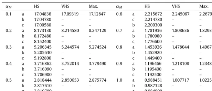
Table 2

TheVSCsζ¯ forHS,VHSwith ω=0.81,and Maxwellmoleculesunderthediffuse-specularBCwithdifferent TMACs.LBEresultsofthepresentpaper,Siewert [34],andWakabayashiet al. [35] aredenotedbya,b,andc, respectively.

αM HS VHS Max. αM HS VHS Max.

0.1 a 17.04836 17.09319 17.12847 0.6 a 2.215672 2.245067 2.267942

b 17.04780 – – c 2.214780 – –

c 17.00580 – – b 2.209300 – –

0.2 a 8.173130 8.214580 8.247129 0.7 a 1.781936 1.808636 1.829366

b 8.172480 – – b 1.780980 – –

c 8.152400 – – c 1.776600 – –

0.3 a 5.206345 5.244574 5.274524 0.8 a 1.453926 1.478044 1.496725

b 5.205630 – – b 1.452920 – –

c 5.192800 – – c 1.449400 – –

0.4 a 3.716862 3.752014 3.779490 0.9 a 1.196466 1.218108 1.234829

b 3.716090 – – b 1.195400 – –

c 3.706900 – – c 1.192500 – –

0.5 a 2.818444 2.850653 2.875774 1.0 a 0.988451 1.007717 1.022560

b 2.817610 – – b 0.987328 – –

c 2.810700 – – c 0.984900 – –

andtheVSCiscalculatedas

¯

ζ

= −

2

−

k1

2P

¯

.

(30)

Inthenumericalsimulation,wefindthat

δ

=

100 isaccurateenoughtorecovertheKLFandVSC,whencomparedtothe solutionof

δ

=

1000.However,when

δ

=

10,thatis,thedistancebetweentwoplatesisroughly10timesofthemeanfree path,twoKnudsenlayersinteractwitheachother,whichleadstoaninaccurateKLFbyusingEq. (29).

4.1. Theviscousslipcoefficient

Althougha large number ofVSCs havebeen computedfromkinetic model equations [7], veryfew data are available basedontheLBEforvariousintermolecularpotentials.Inthissection,westudyhowtheintermolecularpotentials(including theinversepower-law,shieldedCoulomb,andLennard-Jonespotentials)andgas-kineticBCs(includingthediffuse-specular andCercignani–LampisBCs)affecttheKramer’sproblem.

4.1.1. Theinfluencesofintermolecularpotentialandgas-kineticBC

Table 2 tabulates the VSCs obtained from the LBE for HS, variable hard-sphere (VHS) with

ω

=

0

.

81, and Maxwell molecules, when thediffuse-specular BC ofdifferent TMACs is used.Results of Wakabayashi et al. [35] using a discrete velocitymethodandSiewert [34] usingapolynomialexpansiontechniquetosolvetheLBEforHSmoleculesarealsolisted for comparison. It is noticed that the three groupsof data agree well witheach other, especially the relative difference betweenour resultsandthose ofSiewert [34] is lessthan 10−4_{.As expected, theVSC increases astheTMACdecreases.} Also,theVSCisinsensitivetotheintermolecularpotential,whichonlyslightlyincreaseswiththeviscosityindex

ω

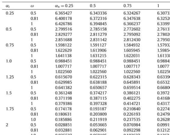
,where therelativedifferencebetweenHSandMaxwellmoleculesislessthan4%.Theseresultsconfirmthestatementinprevious studies [5,7,36].

InordertostudytheKramer’sproblemwithamoresophisticatedgas-surfaceinteraction,theLBEisthensolvedwiththe Cercignani–Lampis BC.Resultsare summarizedinTable 3,fortheeffectiveTMAC

αt

∈ [

0

.

25

,

2

]

andtheenergy accommo-dationcoefficient

αn

∈ [

0

.

25

,

1

]

.Whenthevalueof

αn

andtheintermolecularpotentialarefixed,theVSCincreasesrapidly when

αt

decreases,whichisconsistentwiththatinthediffuse-specularBC.Theadditionalfreeparameter

αn

inCercignani– LampisBCintroduces newinteresting results.When

αt

<

1,forafixed

αt

andintermolecularpotential,theVSCdecreases slightlyas

αn

increases, wherethemaximumdropintheVSC islessthan 2%.When

αt

=

1,theCercignani–Lampis BCis reducedtothefullydiffuseoneinthisproblem,andtheVSCdoesnotvarywith

αn

.When

αt

>

1,thevariationofVSCon

αn

reversescomparedtothatof

αt

<

1;anditisstronglyinfluencedby

αn

,especiallywhen

αt

islarge.Forinstance,forHS moleculesat

αt

=

2,theVSCisincreasedbymorethanthreetimeswhen

αn

changesfrom0

.

25 to1.Forfixed

αn

and

αt

, thechangeintheVSCisinsensitivetotheintermolecularpotentialswhen

αt

1

.

75.However,when

αt

isclosetotwo(i.e. the“backward”scattering),theinfluenceoftheintermolecularpotentialbecomes considerable.Forexample,when

αt

=

2 and

αn

=

1,MaxwellmoleculeshaveaVSCthatisabout37%higherthanthatforHSmolecules.

4.1.2. TheviscousslipcoefficientasafunctionoftheeffectiveTMAC

ThevariationofVSCwithrespecttotheeffectiveTMAC

α

(fordiffuse-specularandCercignani–LampisBCs,

α

=

αM

and

[image:10.561.133.416.87.311.2]

Table 3

TheVSCforHS,VHSwithω=0.81,andMaxwellmoleculesunderCercignani–LampisBCwith differenteffectiveTMACαtandenergyaccommodationcoefficientαn.

αt ω αn=0.25 0.5 0.75 1

[image:10.561.135.415.354.500.2]

0.25 0.5 6.365427 6.343336 6.324267 6.307321 0.81 6.400178 6.372316 6.347638 6.325202 1 6.426786 6.394845 6.366237 6.339971 0.5 0.5 2.799516 2.785158 2.772602 2.761338 0.81 2.829277 2.811279 2.795092 2.780207 1 2.851688 2.831142 2.812430 2.795028 0.75 0.5 1.598122 1.591127 1.584932 1.579323 0.81 1.622629 1.613906 1.605945 1.598540 1 1.641138 1.631215 1.622031 1.613380 1.0 0.5 0.988451 0.988451 0.988451 0.988451 0.81 1.007717 1.007717 1.007717 1.007717 1 1.022560 1.022560 1.022560 1.022560 1.25 0.5 0.615670 0.622315 0.628343 0.633906 0.81 0.629985 0.638188 0.645891 0.653221 1 0.641382 0.650657 0.659514 0.668067 1.5 0.5 0.361248 0.374217 0.386121 0.397213 0.81 0.371198 0.387115 0.402275 0.416866 1 0.379386 0.397328 0.414721 0.431729 1.75 0.5 0.174178 0.193187 0.210840 0.227456 0.81 0.180631 0.203809 0.226193 0.247988 1.0 0.185886 0.211919 0.237535 0.262897 2 0.5 0.028851 0.053665 0.076984 0.099153 0.81 0.032881 0.062901 0.092298 0.121255 1.0 0.035527 0.069105 0.102637 0.136246

Table 4

FittingcoefficientsinEq. (31) forHS,VHSwithω=0.81,andMaxwellmoleculesunderthe diffuse-specularandCercignani–LampisBCs.

BC αn ω a b·10 c

Diffuse-specular n/a 0.5 1.773 1.1660 0.6687 n/a 0.81 1.773 1.4270 0.6238

n/a 1 1.773 1.6370 0.5885

Cercignani–Lampis 0.25 0.5 1.774 0.7266 0.7127 0.81 1.775 0.8889 0.6781

1 1.776 1.0130 0.6516

Cercignani–Lampis 0.5 0.5 1.773 0.4772 0.7367 0.81 1.774 0.5867 0.7069

1 1.774 0.5742 0.6837

Cercignani–Lampis 0.75 0.5 1.772 0.2434 0.7597 0.81 1.773 0.2915 0.7358

1 1.773 0.3373 0.7164

Cercignani–Lampis 1.0 0.5 1.772 0.0218 0.7818 0.81 1.766 0.0543 0.7370

1 1.772 0.0000 0.7499

WefindfromTables2and3thattheVSCcanbefittedbyageneralfunctionastheoneusedbyLilley&Sader [11] for bothdiffuse-specularandCercignani–LampisBCs:

¯

ζ (

α

)

=

a

α

−

b

α

−

c

,

(31)

wherethefittingcoefficientsa

,

b,andcareshowninTable4fortypicalinversepower-lawintermolecularpotentials.Fig.4

shows that the fitted curve (constructed from the datawhen

α

≥

0

.

2) can accurately predict the VSC even in thelimit

α

→

0.Forinstance,whentheTMACis0.05,relativedifferencesbetweenthefittedVSCandtheLBEsolutionsarelessthan 0

.

1% forbothdiffuse-specularandCercignani–LampisBCs.

4.2. TheKnudsenlayerfunction

4.2.1. Theinfluenceoftheintermolecularpotential

[image:11.561.91.446.56.188.2]

Fig. 4.TheVSCasafunctionofeffectiveTMACαforHSmolecules,whenthe(a)diffuse-specularBCand(b)Cercignani–LampisBCwithαn=0.25 are used.Solidlines:thenumericalfittingofEq. (31) usingthedatafromtheLBEsolutions(circles).Squares:thedatafromtheLBEbutnousedforfitting. Notethatothervaluesofαnandothertypesofintermolecularpotentialsshowasimilarbehavior.

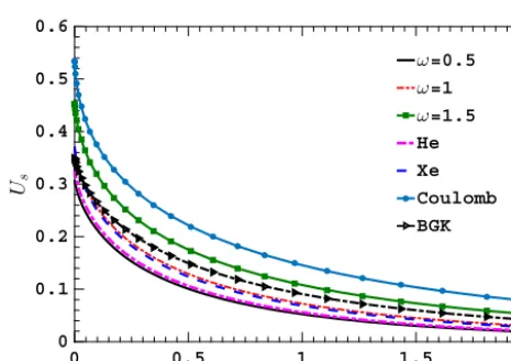
Fig. 5.KLFsfromtheLBEsolutionsfortheinversepower-lawpotentials,theLennard-JonespotentialsofHeliumandXenonwhenthegastemperature is300 K,andtheshieldedCoulombpotentialofchargedmoleculeswhen=kBTw.TheresultfromBGKequationisalsoincludedforcomparison.The diffuseBCisused.

xenonlie betweenthose ofHS andMaxwell molecules.Thisiscomprehensible becausethe effectiveviscosityindexesof heliumandxenon ata temperatureof300 K are0.66and0.85 [38],respectively. TheKLF predictedby theBGK iseven largerthanthatfromtheMaxwellmolecules,butissmallerthanthatof

ω

=

1

.

5 wherethegasmoleculesinteractwithsoft potentials.TheshieldedCoulombpotentialhasthelargestKLF,sinceitseffectiveviscosityiscloseto2.5 [18].

Thus,contrarytotheVSC whosevalueisinsensitivetotheintermolecularpotential,theKLFisstronglyaffectedbythe intermolecularpotential.Thatis,whentheeffectiveviscosityindexincreases,(i) thevalueoftheKLFincreases,and(ii) the KLFdecaysmoreslowly,orequivalently,theKnudsen layerbecomes wider.Forexample,atthesolid surface, therelative differencebetweenKLFsofMaxwellandHSmoleculesisapproximate20%,andthatbetweentheshieldedCoulombandHS potentialsreaches60%.Relativedifferencesatdistances oneto twomeanfree pathaway fromthesolid surface areeven larger,say,whenx2/λ

=

2 thevalueofKLFofshieldedCoulombpotentialisabout4timesofthat ofHSpotential.Onthe otherhand,whenUs isdecreasedto0.01 ofitsvalue atthesolidsurface,thecorrespondingdistancestothesolidsurface

fortheHSandMaxwellmoleculesareabout2

.

7

λ

and3

.

5

λ

,respectively.

4.2.2. Theinfluenceofthegas-kineticBC

Forthesakeofclarity,weonlyfocusonHSmolecules.Thediffuse-specularBCisfirstconsideredinFig.6(a).Itisfound thattheKLFincreasesas

αM

decreases.Forafixed

αM

,theKLFdecreasesrapidlywhenmovingawayfromthesolidsurface, say,itsvaluedecaysbyroughly 85% ofthevalueonthesolidsurfacewhenx2 isaboutonemeanfreepathawayfromthe solidsurface.

[image:11.561.154.387.242.406.2]

[image:12.561.88.460.56.282.2]

Fig. 6.TheKLFforHSmolecules.(a) Thediffuse-specularBC.Alongthearrow,αM=0.2,0.4,0.6,0.8,1.(b) TheCercignani–LampisBCwithαn=0.25. Alongthearrow,αt=0.5,1,1.5 and 2.(c) TheCercignani–LampisBCwithαt=2.Alongthearrow,αn=0.25,0.5,0.75 and 1.Dots:LBEsolutions.Solid lines:fittedcurvesusingEq. (4) with

M

,N=2.Insets:zoomedregionsinthevicinityofthesolidsurface.

Table 5

FittedcoefficientscorrespondingtoEq. (4) with

M

,N=2 fortheKLFobtainedfromtheLBEwithHS,VHSwithω=0.81,and Maxwellmolecules,whenthediffuse-specularBCisused.

ω αM c0,0 c0,1 c0,2 c1,0 c1,1 c1,2·10 c2,0 c2,1 c2,2·102

0.5 0.1 0.6502 1.2720 −0.3624 1.4640 0.9950 −0.6074 −2.0090 0.1593 0.2246 0.2 0.6084 1.1760 −0.3257 1.3260 0.9093 −0.5358 −1.8360 0.1410 0.1967 0.3 0.5675 1.0830 −0.2915 1.1970 0.8283 −0.4699 −1.6720 0.1241 0.1712 0.4 0.5277 0.9941 −0.2598 1.0760 0.7517 −0.4095 −1.5170 0.1085 0.1479 0.5 0.4889 0.9091 −0.2302 0.9630 0.6792 −0.3543 −1.3710 0.0943 0.1267 0.6 0.4509 0.8277 −0.2029 0.8570 0.6108 −0.3040 −1.2330 0.0813 0.1075 0.7 0.4139 0.7498 −0.1776 0.7582 0.5463 −0.2585 −1.1030 0.0695 0.0902 0.8 0.3778 0.6752 −0.1543 0.6661 0.4856 −0.2173 −0.9805 0.0588 0.0748 0.9 0.3424 0.6038 −0.1328 0.5805 0.4284 −0.1805 −0.8652 0.0492 0.0610 1.0 0.3079 0.5356 −0.1132 0.5012 0.3746 −0.1480 −0.7568 0.0406 0.0489 0.81 0.1 0.7436 1.6500 −0.6657 2.3940 1.4840 −1.3430 −3.0070 0.3430 0.5216 0.2 0.6935 1.5130 −0.5949 2.1550 1.3470 −1.1840 −2.7270 0.3030 0.4571 0.3 0.6450 1.3840 −0.5294 1.9330 1.2180 −1.0380 −2.4640 0.2664 0.3983 0.4 0.5980 1.2610 −0.4691 1.7270 1.0980 −0.9046 −2.2190 0.2329 0.3449 0.5 0.5523 1.1450 −0.4135 1.5360 0.9858 −0.7836 −1.9890 0.2024 0.2966 0.6 0.5081 1.0360 −0.3624 1.3590 0.8806 −0.6739 −1.7750 0.1747 0.2531 0.7 0.4651 0.9315 −0.3155 1.1940 0.7823 −0.5747 −1.5750 0.1495 0.2139 0.8 0.4233 0.8331 −0.2727 1.0430 0.6907 −0.4855 −1.3890 0.1269 0.1789 0.9 0.3827 0.7400 −0.2336 0.9035 0.6052 −0.4056 −1.2160 0.1065 0.1478 1.0 0.3433 0.6519 −0.1981 0.7753 0.5257 −0.3345 −1.0550 0.0883 0.1203 1 0.1 0.8123 1.9930 −1.0180 3.3540 1.9460 −2.3230 −4.0160 0.5808 0.9405 0.2 0.7559 1.8180 −0.9055 3.0050 1.7580 −2.0430 −3.6190 0.5118 0.8235 0.3 0.7016 1.6530 −0.8023 2.6820 1.5820 −1.7880 −3.2510 0.4490 0.7174 0.4 0.6491 1.4980 −0.7076 2.3840 1.4190 −1.5570 −2.9100 0.3918 0.6214 0.5 0.5983 1.3530 −0.6210 2.1090 1.2670 −1.3470 −2.5930 0.3400 0.5349 0.6 0.5493 1.2170 −0.5419 1.8570 1.1260 −1.1580 −2.3000 0.2931 0.4571 0.7 0.5019 1.0880 −0.4699 1.6240 0.9955 −0.9880 −2.0290 0.2508 0.3874 0.8 0.4560 0.9682 −0.4044 1.4120 0.8745 −0.8354 −1.7790 0.2127 0.3252 0.9 0.4116 0.8553 −0.3450 1.2170 0.7625 −0.6991 −1.5480 0.1787 0.2700 1.0 0.3685 0.7495 −0.2914 1.0390 0.6590 −0.9010 −1.3350 0.1483 0.2212

[image:12.561.80.472.371.643.2]

[image:13.561.71.468.86.352.2]

Table 6

FittingcoefficientscorrespondingtoEq. (4) with

M

,N=2 fortheLBEsolutionsofKLF,whenHSmoleculesandCercignani–Lampis BCareused.SincetheKLFisindependentofαnwhenαt=1,onlythefittingcoefficientsforαt=1 andαn=0.25 aretabulated.

αn αt c0,0 c0,1 c0,2 c1,0 c1,1 c1,2×10 c2,0 c2,1×10 c2,2×103

0.25 0.25 0.4756 0.7342 −0.1390 0.5628 0.4537 −0.2119 −0.9529 0.5551 0.7804 0.5 0.4174 0.6648 −0.1299 0.5416 0.4265 −0.1888 −0.8847 0.5012 0.6781 0.75 0.3616 0.5988 −0.1214 0.5210 0.4001 −0.1676 −0.8195 0.4520 0.5814 1 0.3079 0.5356 −0.1132 0.5012 0.3746 −0.1476 −0.7568 0.4056 0.4893 1.25 0.2559 0.4746 −0.1053 0.4823 0.3501 −0.1283 −0.6965 0.3607 0.4004 1.5 0.2051 0.4151 −0.0975 0.4643 0.3265 −0.1089 −0.6379 0.3156 0.3134 1.75 0.1551 0.3563 −0.0897 0.4473 0.3037 −0.0891 −0.5806 0.2687 0.2270 2 0.1056 0.2980 −0.0816 0.4316 0.2818 −0.0683 −0.5245 0.2188 0.1405 0.5 0.25 0.4080 0.6424 −0.1285 0.5242 0.4152 −0.1848 −0.8585 0.4961 0.6048 0.5 0.3735 0.6048 −0.1231 0.5159 0.4011 −0.1714 −0.8228 0.4635 0.5872 0.75 0.3403 0.5694 −0.1180 0.5084 0.3877 −0.1592 −0.7891 0.4338 0.5372 1.25 0.2762 0.5023 −0.1085 0.4942 0.3619 −0.1363 −0.7252 0.3781 0.4524 1.5 0.2446 0.4689 −0.1037 0.4871 0.3491 −0.1247 −0.6934 0.3498 0.3951 1.75 0.2130 0.4345 −0.0987 0.4797 0.3363 −0.1124 −0.6608 0.3198 0.3462 2 0.1810 0.3987 −0.0935 0.4719 0.3232 −0.0992 −0.6271 0.2873 0.2953 0.75 0.25 0.3545 0.5836 −0.1203 0.5099 0.3926 −0.1647 −0.8019 0.4479 0.5554 0.5 0.3383 0.5658 −0.1177 0.5061 0.3861 −0.1582 −0.7852 0.4319 0.5304 0.75 0.3229 0.5502 −0.1154 0.5034 0.3802 −0.1526 −0.7705 0.4182 0.5090 1.25 0.2931 0.5211 −0.1111 0.499 0.3691 −0.1426 −0.7433 0.3932 0.4698 1.5 0.2780 0.5058 −0.1088 0.4964 0.3634 −0.1372 −0.7290 0.3798 0.4489 1.75 0.2625 0.4888 −0.1063 0.4929 0.3572 −0.1310 −0.7130 0.3645 0.4251 2 0.2462 0.4696 −0.1035 0.4884 0.3504 −0.1238 −0.6951 0.3466 0.3979 1 0.25 0.3093 0.5405 −0.1138 0.504 0.3762 −0.1499 −0.7617 0.4109 0.4980 0.5 0.3083 0.5370 −0.1134 0.5020 0.3751 −0.1483 −0.7582 0.4071 0.4918 0.75 0.3080 0.5357 −0.1132 0.5013 0.3747 −0.1477 −0.7570 0.4058 0.4896 1.25 0.3079 0.5354 −0.1132 0.5011 0.3746 −0.1475 −0.7567 0.4055 0.4890 1.5 0.3075 0.5342 −0.1130 0.5004 0.3742 −0.1470 −0.7555 0.4042 0.4869 1.75 0.3066 0.5311 −0.1127 0.4987 0.3732 −0.1455 −0.7524 0.4008 0.4813 2 0.3050 0.5255 −0.1120 0.4955 0.3715 −0.1430 −0.7469 0.3949 0.4714

4.2.3. FittingtheKnudsenlayerfunctionandthesingularityofvelocitygradient

The KLFis essentialnot only indetermining thenonlinear constitutionin theKnudsen layer [8], butalso indefining the singularity of velocity gradient nearthe solid surface. In a recent work based on theBGK model,Jiang & Luo have rigorouslyshownthatthevelocitynearthesolidsurfacecanbedescribedbyEq. (4),whosegradientpossessesalogarithmic divergence [14].Intheirwork,itwasnumericallydemonstratedthatthefirstfourleadingtermsofEq. (4) cancapturethe velocityprofileinanextremelysmallinterval 0

≤

x2

≤

1

.

5

×

10−7.However,noattemptismadetofitthevelocityprofile outsidetheindicatedregion.

Inthiswork,based onthehighly accurateresultsofthe LBE,wefindthat theentireKLFcanbe describedby Eq. (4), provided that more high-order terms are included. The associated fitting coefficients in Eq. (4) with M

,

N

=

2 for the diffuse-specularandCercignani–Lampis BCsaretabulated inTables 5and6,respectively. Wenote that when

αn

isfixed, theabsolutevalueoffittingcoefficient decreasesas

αt

increases.Meanwhile,thedependencyofeachfittingcoefficienton

αt

becomesweakerandweakeras

αn

increases.Forinstance,when

αn

isincreasedfrom0.25to1,themaximumrelative differenceinc0,0 fordifferent

αt

isreducedfrom350% to2%.FromtheinsetsinFig.6,we observethat thefittedcurves agreequitewellwiththenumericalresults.NotethatEq. (4) withM

,

N

=

2 canalsodescribetheKLFverywellwhenthe distancetothesolidsurfacereaches10

λ

.

Next, the singularity of velocity gradient in the vicinity of the solid surface is investigated through the deviation of Eq. (4) withrespecttox2.Thissingularityisdominatedbythetermwithn

=

0 andm

=

1 inEq. (4),thatis,thevelocity gradientnearthesolidsurfaceisc0,1lnx2 [12,14].FromTable5,itisfoundthatforafixedTMAC, c0,1 increaseswiththe viscosityindex,indicatingthattherateofdivergenceisfasterforthegasmoleculeswithalargervalueofviscosityindex, see Fig.7. However, thistrend reverse atx2

≈

0

.

015

λ

. Thisbehavior is somehowrelated tothe variation of equilibrium collision frequency

νeq

. From the left insetin Fig. 7 we see that, when the rarefaction parameter

δ

is fixed,

νeq

(

0

,

0

,

0

)

increaseswiththeviscosityindex

ω

,whichmeansthatthecollisionfrequencyislargerforlargervaluesof

ω

,sothatthe gasapproachestotheequilibriumquickerandhencethevelocitydefectdecreasesfaster.Similarly,thevelocitygradientat x2

>

0

.

015

λ

seemstobe proportionalto

νeq

(

0

,

v2

>

3

,

0

)

.Itshouldbe notedthat,however,thisexplanationisonlybased onthenumericalfinding;onemayresorttotherigorousmathematicalanalysistohaveadeepunderstanding [12,39].When theintermolecularpotentialisfixed,a smallereffectiveTMACwillproducealargervelocitygradientnearthesolidsurface, seeTables5and6.

4.2.4. ThesimilarityoftheKnudsenlayerfunction

[image:14.561.114.435.57.238.2]

Fig. 7.Theabsolutevalueofvelocitygradient|λdUs/dx2|forHS(solidline),Maxwell(dash-dotline),andsoft-potentialwithω=1.5 (dashline)molecules,

whenthediffuseboundaryisused.Insetsarethezoomedvelocitygradientandtheequilibriumcollisionfrequencyνeq(0,v2,0)normalizedbythe

[image:14.561.144.406.290.469.2]

rarefac-tionparameterδ.

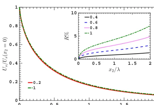
Fig. 8.TherescaledKLF

U

s/Us(x2=0)forαM=0.2 and1,whentheHSmoleculesandthediffuse-specularBCareused.Forclarity,resultsatothervalues ofαMarenotshown.Inset:therelativedifference(R%)of

U

s/Us(x2=0)forvariousαMcomparedtothatofαM=0.2.

Table 7

FittingcoefficientsoftherescaledKLF

U

s/Us(0)forinversepower-lawpotentialswithdifferentvaluesofviscosity indexω,whenthediffuseBCisused.

ω c0,0 c0,1 c0,2 c1,0 c1,1 c1,2·10 c2,0 c2,1 c2,2·102

0.5 1.0000 1.739 −0.3677 1.628 1.217 −0.4794 −2.458 0.1317 0.1589 0.75 1.0000 1.864 −0.5256 2.113 1.462 −0.8429 −2.932 0.2245 0.2976 1 1.0000 2.034 −0.7907 2.820 1.788 −1.5680 −3.623 0.4024 0.6003 1.25 1.0000 2.275 −1.2390 3.864 2.217 −2.9800 −4.648 0.7380 1.2300 1.5 1.0000 2.807 −2.5280 6.238 2.821 −8.4950 −6.999 1.9310 4.4710

We first studythe KLF normalizedby its value on thesolid surface x2

=

0, when the HS moleculesandthe diffuse-specularBCareused.Resultsofothertypesofmoleculesaresimilar.Fig.8showstherescaledKLFUs

/

Us

(

x2

=

0

)

andtheir relativedifferenceatdifferentTMAC,whencomparedwiththatat

αM

=

0

.

2.WenoticethattherescaledKLFfor

αM

=

0

.

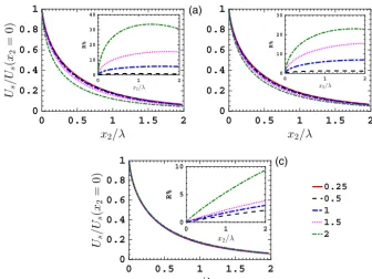
2 and1almost overlap;asshowninthe insetofFig.8,themaximumrelativedifference amongallTMACsislessthan7%. Thus,theKLFfordiffuse-specularBCpossessesagoodsimilaritybetweendifferentvaluesofTMAC.

[image:14.561.105.447.544.603.2]

[image:15.561.101.437.54.306.2] [image:15.561.186.356.393.453.2]

Fig. 9.TherescaledKLF

U

s/Us(x2=0)ofHSmoleculeswhen(a)αn=0.25,(b)αn=0.5,and(c)αn=1,whentheCercignani–LampisBCwithαt= 0.25,0.5,1.0,1.5,and2.0areused.Inset:therelativedifference(R%)of

U

s/Us(x2=0)atvariousTMAC,whencomparedtothatofαt=0.25.

Table 8

Fittingcoefficients ofthe velocitydefect

U

s(0) at the solidsurfacebyEq. (31) forinversepower-law poten-tialswithdifferentvaluesofviscosityindexω,whenthe diffuse-specularBCisused.

ω c1 c2 c3

0.5 1.798 0.2410 −1.1050 0.75 1.776 0.2825 −1.0030 1 1.750 0.3378 −0.8800 1.25 1.820 0.3822 −0.8353 1.5 1.895 0.4368 −0.7721

αn

=

0

.

25,themaximumrelative differencefor

αt

=

2 is about30%,ascomparedwith

αt

=

0

.

25, seetheinsetinFig. 9. Nevertheless,itshouldbenotedthat,forall

αn

with

αt

≤

1,therelativedifferenceoftherescaledKLFislessthan7%.

Approximately,the KLFs isdefined tohave similarityif therelative difference of therescaled KLF fordifferentTMAC is lessthan 10%. Therefore,as showninFigs. 8 and9, the KLFhas thesimilarity when thediffuse-specular BC andthe Cercignani–LampisBCwith

αn

=

1 areconsidered,inthefullrangeofeffectiveTMAC;forCercignani–LampisBCwithother valuesof

αn

,thesimilarityispreservedwhen

αt

≤

1.

Under the diffuse-specular BC, the rescaled KLF can be fitted using Eq. (4), withthe fitting coefficients for different intermolecularpotentialstabulatedinTable7.Furthermore,thecorrespondingKLFonthesolidsurfacex2

=

0 canbefitted usinganexponentialfunctionoftheeffectiveTMAC

α

as

Us(x2

=

0

)

=

c1exp

(

−

c2

α

)

+

c3

,

(32)

wherec1,c2andc3arethefittingcoefficientstabulatedinTable8fordifferentintermolecularpotentials.Asaconsequence, the KLF at arbitrary TMACcan be roughly estimated by multiplying Eq. (32) and the rescaled KLF, withthe maximum relativeerrorbeingsmallerthan 10%.TheKLFfortheCercignani–Lampis BCcanalsobe rescaledaccordingto thedatain Table6.

5. Comparisonwiththeexperiment

[image:16.561.144.408.52.218.2]

Fig. 10.ComparisonsoftheKLFsbetweentheexperimentsandtheLBEsolutionwithαt=0.88,whentheairmoleculesofω=0.75 andvarious

a

nare applied.Exp. A-1andExp. A-2weremeasuredbyReynoldset al. [15].Thediffuse-specularBCwithαM=0.88 isusedintheBGKmodel.

a kinetic modelwitha variablecollision frequency,a reasonable agreementofthe velocityprofile withtheexperimental data wasobserved [40].Giventheapparentdeficiency ofthemodelequation,resultsfromtheLBEofHSmoleculeswere alsocomparedwiththeexperimentaldata [9].However,allthepreviousworkswerebasedontheHSgaswithanviscosity indexof

ω

=

0

.

5,whileairhasaneffectiveviscosityindexof0.75attheroomtemperature. Moreover,theTMACusedin thenumericalsimulationswasone,whichresultsinaVSCofaboutone,whilethemeasuredTMAChasanaveragevalueof

¯

ζ

Exp

=

1

.

1 (whichhasbeenadjustedbymultiplyingafactorof

√

π

/

2).

Inthissection,wetrytoexplaintheexperimentaldatausingtheLBEsolutionsfortheinversepower-lawpotentialwith

ω

=

0

.

75.Although airis a mixtureof oxygenand nitrogen, we treatit asa single-species monatomicgas, since(i) the molecular massesofoxygen andnitrogenare closeto eachother and(ii) for isothermal flow theVSC (or themassflow rate)isinsensitivetotherotationaldegreesoffreedom [41,42].

Fig. 10showsthe KLFobtainedfromtheLBEwith

αt

=

0

.

95,and

αn

=

0

.

1 and 1undertheCercignani–Lampis BC,as wellastheexperimentaldata.TheresultfromtheBGKequationisalsoincludedforcomparison.WeusethevalueofTMAC

α

=

0

.

95,asour numericalcalculation inthe previous section suggeststhat thepredictedVSC fromthe LBEagrees well with the experimental value of 1.1 [15]. It is found that the KLF changes slightlyunder different

αn

, andthe results of

αn

=

1 seemsbetterthantheothersinagreementwiththeexperimentaldata,whilethesolutionoftheBGKequationhas avisibledeviationfromtheexperimentalresults.Notethat whenusingthediffuse-specularBC,similarresultscanalsobe obtainedfor

αM

=

0

.

95.

We note that theKLFfromthe experimentsare scattered,which isinconsistent withthetheoretical analysisthatthe normalized velocity near the solid surface should be independent of the mean free path and shear gradient. Reynolds et al. [15] arguedthat themostpossible reasonwas theinaccuratedetermination ofthemeanfreepath.Therefore, intu-itively,inordertointerprettheexperimental results,oneshouldtakethisfactorintoaccount.Tothisend,wefirstassume the actual TMAC forthe interaction ofair withthe polishedaluminum plate is

αM

in the diffuse-specularBC. Then we calculatetheVSC

ζ (

¯

αM

)

fromtheLBE.If

ζ

¯

Exp

<

ζ (

¯

αM

)

,themeanfreepathintheexperimenthasbeenoverestimateddue

totheinaccuratemeasuringofthegaspressure.Therefore,thevalueoftheKLFfromtheexperiment [15] shouldbe multi-pliedby1

/

σ

= ¯

ζ (

αM

)/

ζ

¯

Exp,whilethewidthoftheKLFshouldbestretchedbyafactorof1

/

σ

.Inthenumericalsimulation,

variousvaluesof

αM

areattempted,untilgoodagreementbetweentheresultsofexperimentandnumericalsimulationare achieved.

Toshow all theresultsinone figure,however,theKLF Us

(

x2)obtainedfromthenumericalsimulation oftheLBEhas

beenrescaledto

σ

Us

(

σ

x2).ComparisonsbetweenthenumericalandexperimentalresultsaredepictedinFig.11.Itisseen

that, whenthe TMACvariesfrom0.8to1,the resultsofLBEcan coveralmostall theexperimental data.Inother words, theTMACofaluminumplateusedintheairexperimentsismostlikely0

.

9

±

0

.

1.IftheTMACis0.9,wehave

σ

=

0

.

9,this meansthatthemeanfreepathintheexperimentisoverestimatedby 10%,whichseemsreasonableduetotheaccuracyof themicro-manometersatthattime.

6. Conclusions

[image:17.561.138.404.53.233.2]

Fig. 11.ComparisonsoftheKLFbetweentheexperimentsandtheLBEsolutionwithαM=0.8,0.9 and 1,whentheairmoleculeswithω=0.75 areused. TheLBEresultsarescaledbyafactorσ= ¯ζExp/ζ (¯αM),whereζ¯Exp=1.1 istheaverageVSCfromtheexperiments.Exp. A-1andExp. A-2aremeasured by [15].

on theBhatnagar–Gross–Krook kinetic model, thesynthetic iteration schemeis assessed tobe accurate at leastwithsix significantdigits.

With this efficient and accurate method, the influences of the intermolecular potentials (i.e. the inverse power-law, Lennard-Jones, andshieldedCoulomb potentials) andkinetic boundaryBCs onthe Knudsen layerhave beeninvestigated basedonthelinearizedBoltzmannequation,wheretheBoltzmanncollisionoperatorforgeneralintermolecularpotentialsis solvedbythefastspectralmethod.Boththediffuse-specularandCercignani–Lampisboundaryconditionsareconsidered.It hasbeenfoundthat,althoughdifferentintermolecularpotentialsleadtoroughlythesamevalueofviscousslipcoefficient, theKLFisstronglyaffectedbythepotential,whosevalueandwidthincreasewiththeeffectiveviscosityindexofgas.

Thehighly accurateVSC anditsgeneralrelationtotheTMACarepresentedfordifferentintermolecularpotentialsand gas-surfaceboundaryconditions.Inaddition,theKLFisfoundtobeperfectlyfittedbytheseries

2_n=0

_m2₌₀cn,mxn

(

xlnx

)

m,

where x is the distanceto the solid surface. Correspondingly, based on the obtainedKLF, the macroscopic flow velocity gradientexhibitsalogarithmicdivergenceontheboundary.Thestrengthofthisdivergencedependsonthecoefficientc0,1, whosevaluealsoincreaseswiththeviscosityindex.Furthermore,thesimilarityoftheKLFhasbeenestablishedbyrescaling theKLFbythedefectvelocityatthesolidsurface.Consequently,theKLFatarbitraryTMACcanbepredictedbymultiplying the rescaledKLF andthedefectvelocity atthe solid surface whichis accuratelyfitted byan exponential function ofthe TMAC.Theseresultsare usefultoformulatetheeffectiveshearviscosity [8] andslipboundarycondition tobeusedinthe frameworkofNavier–Stokesequations [2].

The experimental data of the viscous slip coefficient and KLF measured by [15] has been interpreted fairly well by thelinearizedBoltzmannequation witharealistic viscosityindex. Weconcludedthat theTMACfortheinteractionofair withthepolishedaluminumismostlikely0

.

9

±

0

.

1,insteadof1

.

0 as usedinprevious studiesforacomparisonwiththe experiment.Thisresultsuggeststhatmeanfreepathintheexperimenthasbeenoverestimatedbyabout10%.

Finally,itshouldbe notedthattheaccurateandefficientsyntheticiterativeschemedevelopedinthispaperarereadily to be extended to multi-species gas mixtures [24]. The influence of intermolecular potentials and gas kinetic boundary conditionsontheKramer’sproblemofgasmixturesaresubjecttofuturestudies.

Acknowledgements

This work is founded by jointproject from the Royal Society of Edinburgh and NationalNatural Science Foundation of China under Grant No. 51711530130, the Carnegie Research Incentive Grant forthe Universities in Scotland, andthe EngineeringandPhysicalSciencesResearchCouncil(EPSRC)intheUKundergrantEP/R041938/1.

References

[1]H.A. Kramers, On the behaviour of a gas near a wall, Nuovo Cimento 6 (1949) 297–304.

[2]D.A. Lockerby, J.M. Reese, On the modelling of isothermal gas flows at the microscale, J. Fluid Mech. 604 (2008) 235–261. [3]J.C. Maxwell, VII. On stresses in rarified gases arising from inequalities of temperature, Proc. R. Soc. Lond. 170 (1879) 231–256.

[4]S.K. Loyalka, Momentum and temperature-slip coefficients with arbitrary accommodation at the surface, J. Chem. Phys. 48 (1968) 5432–5436. [5]F. Sharipov, V. Seleznev, Data on internal rarefied gas flows, J. Phys. Chem. Ref. Data 27 (1998) 657–706.

[6]S. Loyalka, Slip and jump coefficients for rarefied gas flows: variational results for Lennard-Jones and n(r)-6 potentials, Physica A 163 (3) (1990) 813–821.