A versatile lattice Boltzmann model for immiscible ternary fluid flows

A versatile lattice Boltzmann model for immiscible ternary

fluid flows

Yuan Yua, Haihu Liub,∗, Dong Lianga,c, Yonghao Zhangd a_{School of Engineering, Sun Yat-Sen University, Guangzhou 510006, China} b_{School of Energy and Power Engineering, Xi’an Jiaotong University, Xi’an 710049, China} c_{Guangdong Provincial Key Laboratory of Fire Science and Technology, Guangzhou 51006, China} d_{Department of Mechanical and Aerospace Engineering, University of Strathclyde, Glasgow G1 1XJ,}

United Kingdom

Abstract

We propose a lattice Boltzmann color-gradient model for immiscible ternary fluid flows, which is applicable to the fluids with a full range of interfacial tensions, es-pecially in near-critical and critical states. An interfacial force for N-phase systems is derived based on the previously developed perturbation operator and is then introduced into the model using a body force scheme, which helps reduce spurious velocities. A generalized recoloring algorithm is applied to produce phase segregation and ensure immiscibility of three different fluids, where a novel form of segregation parameters is proposed by considering the existence of Neumann’s triangle and the effect of equilib-rium contact angle in three-phase junction. The proposed model is first validated with three typical examples, namely the interface capturing for two separate static droplets, the Young-Laplace test for a compound droplet, and the spreading of a droplet between two stratified fluids. This model is then used to study the structure and stability of dou-ble droplets in a static matrix. Consistent with the theoretical stability diagram, seven possible equilibrium morphologies are successfully reproduced by adjusting two ratios of the interfacial tensions. By simulating Janus droplets in various geometric config-urations, the model is shown to be accurate when three interfacial tensions satisfy a Neumann’s triangle. In addition, we also simulate the near-critical and critical states of double droplets where the outcomes are very sensitive to the model accuracy. Our results show that the present model is advantageous to three-phase flow simulations, and allows for accurate simulation of near-critical and critical states.

Keywords: Immiscible multiphase flows, full range of interfacial tensions, color-gradient model, double emulsion droplets, near-critical and critical states

∗_{Corresponding author: Tel.:+86 (0) 298 266 5700;}

Email address:haihu.liu@mail.xjtu.edu.cn(Haihu Liu)

1. Introduction

An emulsion is a mixture of a dispersed phase as droplets in another immiscible fluid that forms a continuous phase. Two basic types of emulsions are the oil-in-water (O/W) and water-in-oil (W/O) emulsions[1]. Recently, more complex systems referred to as double emulsions and Janus emulsions have received a rapidly growing interest due to their unique properties[2, 3, 4] and potential applications[5, 6, 7, 8, 9, 10]. Dou-ble emulsions, also known as ‘emulsion of emulsion’ or ‘emulsion within emulsion’, are emulsions with smaller droplets encapsulated in larger droplets. The shell fluid can serve as a barrier between the core droplets and the outer environment, which makes double emulsions highly desirable for applications in controlled release, separation, and encapsulation[1, 2, 3, 4]. Janus emulsions, which are named after the two-faced Roman god Janus, are highly structured fluids consisting of emulsion droplets that have two distinct physical properties[11]. Because of their natural asymmetric abil-ity in the compositions and the shapes, Janus emulsions are often used in the fields that need asymmetry in the shape and the materials. In the applications of emulsions, morphology is one of the most important properties and closely related to other emul-sion properties such as rheology, droplet size, relative stability, electrical conductivity and zeta potential[2, 3, 4, 12]. A number of theoretical and experimental studies have been devoted to identifying different equilibrium morphologies and their transforma-tion. For example, Torza and Mason[13] studied the droplet morphology in terms of spreading coefficients and obtained the theoretical relationship between the droplet morphology and spreading coefficients. They experimentally observed three equilib-rium morphologies of double droplets, i.e. complete engulfing, partial engulfing and non-engulfing, which correspond to three sets of spreading coefficients. Beyond these three equilibrium states, Pannacci et al.[14] identified several new morphologies of double droplets, and found the non-equilibrium morphologies can have long lifetimes controlled by hydrodynamics, which facilitates the use of double droplets to produce encapsulated particles at early times and Janus particles at longer times. Guzowski et al.[15] presented a detailed theoretical analysis on the possible equilibrium morpholo-gies of double droplets and designed the structure of double emulsions by tuning the volumes of the constituent segments experimentally. As a supplement to theoretical and experimental studies, numerical modelling and simulations are becoming increas-ingly popular in investigation of the behavior of Janus/double emulsions, which are typical of three-phase flow problems.

flow problem[28].

In the past decades, the lattice Boltzmann (LB) method has developed into a promis-ing alternative to the traditional Navier-Stokes-based solvers, for simulatpromis-ing complex flow problems. It is a pseudo-molecular method tracking evolution of the distribu-tion funcdistribu-tion of an assembly of molecules, built upon microscopic models and meso-scopic kinetic equations[29]. The LB method has several advantages over the tradi-tional Navier-Stokes-based solvers, e.g. the algorithm simplicity and parallelizability, and the ease of handling complex boundaries[30]. In addition, its kinetic nature allows a simple incorporation of microscopic physics without suffering from the limitations in terms of length and time scales typical of molecular dynamics simulations[31]. Thus, the LB method is particularly useful in the simulation of multiphase flows. The existing LB models for multiphase flows can be generally classified into four categories: color-gradient model[32, 33, 28], interparticle-potential model[34, 35, 36, 37, 38], phase-field-based model[39, 40, 41], and mean-field theory model[42]. These models have shown great success as in dealing with two-phase flow problems, and all of them except the mean-field theory model have been extended to the modeling of immiscible ternary fluids, see, e.g. Refs[43, 44, 45, 46, 47, 48, 49, 50, 51]. The ternary color-gradient models[49, 50] inherit a series of advantages of its two-phase counterpart, such as strict mass conservation for each fluid, flexibly tunable interfacial tensions, and the stability for a broad range of viscosity ratios, and they are well suited to exploring the dynamic processes occurring in ternary fluid systems as previously demonstrated by Fu et al.[51] and Jiang et al.[52]. The existing color-gradient models, however, commonly suffer from a problem, i.e. three interfacial tensions should satisfy a Neumann’s trian-gle. In industrial processes, surfactants are often added to emulsions to stabilize them against droplet coalescence. The presence of surfactants could significantly modify the interfacial tensions so that the interfacial tensions do not always yield a Neumann’s triangle. To correctly predict the dynamical behavior of emulsions, thereby allowing precise control over the droplet geometry and composition, it is necessary for a nu-merical model to be capable of simulating ternary fluids with a full range of interfacial tensions. On the other hand, it is challenging to simulate the near-critical and critical states of a ternary fluid system where the largest interfacial tension is close to the sum of the other two, as the outcomes are very sensitive to the model accuracy.

2. Numerical method

The two-phase color-gradient LB model of Liu et al.[28, 53] is extended to the simulation of immiscible ternary fluids. The ternary color-gradient model consists of three steps, i.e. the collision step, the recoloring step and the streaming step. In the collision step, an interfacial force that describes the interactions among different fluids is derived from the perturbation operator presented in Leclaire et al.[50], and is then introduced by the body force scheme of Guo et al.[54] In the recoloring step, a novel form of segregation parameters is proposed to ensure accurate phase segregation in three-phase junction and allow for the states where three interfacial tensions between the fluids cannot form a triangle, known as the Neumann’s triangle. The distribution functions fi,r, fi,g and fi,b are introduced to represent three immiscible fluids, i.e. red

fluid, green fluid and blue fluid, where the subscriptiis the lattice velocity direction and ranges from 0 to (n-1) for a givenm-dimensional DmQnlattice model. The total distribution function is defined as fi = Pkfi,k (k = r, g or b), which undergoes a

collision step as

f_i†(x,t)= fi(x,t)+ Ωi(x,t)+ Φi(x,t), (1)

wherefi(x,t) is the total distribution function in thei-th velocity direction at the

posi-tionxand the timet, f_i†is the post-collision distribution function,Ωiis the

Bhatnagar-Gross-Krook (BGK) collision operator, andΦiis the forcing term (also known as

per-turbation operator), which contributes to the mixed interfacial regions and creates the interfacial tensions between different fluids.

In the BGK collision operator, the total distribution functions are relaxed toward a local equilibrium with a single relaxation time:

Ωi(x,t)=−

1

τf

h

fi(x,t)−f eq i (x,t)

i

, (2)

whereτf is the dimensionless relaxation time, and f eq

i is the equilibrium distribution

function of fi. The equilibrium distribution function is obtained by a second order

Taylor expansion of Maxwell-Boltzmann distribution with respect to the local fluid velocityu:

f_ieq=wiρ

"

1+ei·u

c2

s

+(ei·u)2

2c4

s

−u·u 2c2

s

#

, (3)

whereρ=P

kρkis the total density andρkis the density of the fluidk;csis the speed of

sound;eiis the lattice velocity in thei-th direction; andwiis the weighting factor. For

the two-dimensional nine-velocity (D2Q9) model,ei is defined ase0 =(0,0),e1,3 = (±c,0),e2,4 = (0,±c),e5,7 =(±c,±c), ande6,8 =(∓c,±c), wherec =δx/δt =

√ 3cs

withδx andδt being the lattice spacing and time step, respectively (for the sake of

simplicity,δx = δt = 1 is used hereafter);wi is given byw0 = 4/9,w1−4 =1/9 and

w5−8=1/36.

the interfacial tensions between different fluids in three-phase simulations. Following Leclaire et al.[50], the perturbation operator is given by

Φi =

X

k

Φi,k, (4)

Φi,k =

X

l,l,k

AklCkl

2 |Gkl| "

wi

(ei·Gkl)2 |Gkl|2

−Bi

#

, (5)

whereGkl= ρ_ρl∇ρ_ρk −ρ_ρk∇ρ_ρl is the color gradient [50] and is introduced to identify the

location of thek-linterface, i.e. the interface between the fluidkand the fluidl. Ckl

is a concentration factor that controls the activation of the interfacial tension at thek-l

interface, and is given by [50]

Ckl=min

     10

6ρkρl

ρ0 kρ 0 l ,1     

, (6)

whereρ0

kis the density of the pure fluidk, andAklis a parameter related to the interfacial

tension between the fluidskandl, i.e. σkl= 1₉(Akl+Alk)τf. The generalized

expres-sion forBiwas given by Liu et al.[28] and it was in particular taken asB0 =−4/27,

B1−4 =2/27 and B5−8 = 5/108 in the work of Leclaire et al.[50]. It is worth noting that Eq.(5) is not limited to the case with ternary fluids, and can be also applicable to

N-phase (N>3) systems.

Using the Chapman-Enskog multiscale analysis, it is shown that the perturbation operator, given by Eqs.(4) and (5), can lead to the following interfacial force:

Fs=−∇ ·

      τfδt

X

i

Φieiei

      = X k X

l,l,k ∇ ·

σ_klCkl

2 |Gkl|(I−nklnkl)

, (7)

wherenklis the unit normal vector of thek-linterface and is defined bynkl=Gkl/|Gkl|.

Instead of using Eqs.(4) and (5), the effect of interfacial tension is realized through the body force scheme of Guo et al.[54], which is able to reduce effectively spurious velocities while keeping high numerical accuracy [53, 55]. According to Guo et al.[54], the forcing termΦiin Eq. (1) is written as

Φi(x,t)=wi 1−

1 2τf

! _e

i−u

c2

s

+ei·u

c4

s

ei

!

·Fs(x,t)δt, (8)

where the local fluid velocity is defined by the averaged momentum before and after the collision, i.e.,

ρu(x,t)=X

i

fi(x,t)ei+

1

2Fs(x,t)δt. (9)

In this work, we assume equal densities for the red, green and blue fluids. To allow for unequal viscosities of the three fluids, we determine the local kinematic viscosityν by a harmonic mean

whereνk(k=R,GorB) is the kinematic viscosity of the fluidk. The local relaxation

timeτf can be calculated from the local viscosity using the following equation:

ν= τf −

1 2 !

c2_sδt. (11)

The partial derivatives in the interfacial forceFsshould be evaluated through

suit-able difference schemes. To minimize the discretization errors, the fourth-order isotropic finite difference scheme

∂αϕ(x,t)= 1

c2

s

X

i

wiϕ(x+eiδt,t)eiα, (12)

is used to evaluate the derivatives of a variableϕ.

Although the forcing term generates the interfacial tensions, it does not guarantee the immiscibility of different fluids. In order to minimize the mixing of the fluids, a recoloring step is applied. Based on the pioneering work of D’Ortona et al.[56], Latva-Kokko and Rothman[57] developed a recoloring algorithm to demix two immiscible fluids, which can overcome the lattice pinning problem and creates a symmetric dis-tribution of particles around the interface so that unphysical spurious velocities can be effectively reduced. This recoloring algorithm was later generalized by Spencer et al.[49] to three-phase fluid flows. Following Spencer et al.[49], the recolored distribu-tion funcdistribu-tions of the fluidk(k=r,gorb) are

f_i‡_,k(x,t)= ρk

ρ f †

i (x,t)+

X

l,l,k

βklwi

ρkρl

ρ nkl·ei, (13)

wheref_i‡_,kis the recolored distribution functions of the fluidk, andβklis a segregation

parameter related to the thickness of thek-linterface. It should be noted thatβkl=βlk

in order to conserve mass and momentum during the recoloring process.

ߪ

ߪ

ߪ

߮௥௚

߮௚௕

߮௥௕

Figure 1: Neumann’s triangle

For the ternary fluids and when three interfacial tensions satisfy a Neumann’s tri-angle (see Fig. 1), the equilibrium contact tri-angleϕklwill be formed between the fluids

in three-phase junction, and it is related to the interfacial tensions by

cos(ϕkl)=

σ2

mk+σ

2

ml−σ

2

kl

2σmkσml

Spencer et al. [49] theoretically showed that in three-phase junction, there should be a relationship betweenϕkland the (relative) interface thickness, which is controlled by

the segregation parameterβkl. Hence, it is of great importance to select a properβklin

three-phase simulations. Several different forms ofβklhave been provided in literature.

Spencer et al. [49] proposed the first expression for the segregation parameters, which is given by

                      

βrg=β0

βrb=β0

"

1+27ρrρgρb

ρ3

sinϕgb−1

#

βgb=β0

"

1+27ρrρgρb

ρ3 (sinϕrb−1) #

, (15)

whereβ0is the reference segregation parameter. Clearly, the segregation parameters in Eq. (15) will degenerate intoβkl=β0at an interface where only two fluids are present.

So it is suggested to takeβ0 =0.7 to be consistent with the segregation parameter in the two-phase color-gradient model[28]. Leclaire et al. [50] improved the segregation parameters of Spencer et al. [49] by settingβkl=β0for the largestϕklin the Neumann’s

triangle,

βkl=

      

β0 _klwithϕ

max

β0_+β0_C

tsin (π−ϕmax−ϕkl)−1 otherwise

, (16)

whereϕmax =max(ϕkl) andCt =min

35ρ_rρ_gρ_b ρ3 ,1

. Leclaire et al.[50] also mentioned to useβkl = β0 when the Neumann’s triangle does not exist. Clearly, Eq. (16) will

degradate to Eq. (15) whenϕmax = ϕrg. Althogh Eqs.(15) and (16) work to some

extent especially when the Neumann’s triangle exists, they cannot accurately simulate the critical state where the largest interfacial tension equals the sum of the other two, which will be shown later. Recently, Fu et al.[51] seemed to have also noticed that Eqs.(15) and (16) do not always produce convincing results in three-phase simulations, so they simply selected a constantβkl, i.e.

βkl=β0. (17)

It is evident that the dependence ofβklonϕklis not considered in Eq.(17), and thus

incorrect results may be obtained, e.g. in the critical state.

To overcome the aforementioned drawbacks associated with the existing βkl, a

novel form of segregation parameters is proposed. First, we determine whether the Neumann’s triangle exists by calculating

Xkl=

σ2

mk+σ

2

ml−σ

2

kl

2σmkσml

. (18)

It is easily seen from Eq.(14) that the Neumann’s triangle will exist if|Xkl|<1 for all

kl. Then, the segregation parameterβklis defined as a continuous function ofXkl:

βkl=β0+β0min

35ρrρgρb

ρ3 ,1 !

where

g(Xkl)=

                

1 Xkl<−1

1−sin (arccos (Xkl)) −1≤Xkl<0

sin (arccos (Xkl))−1 0≤Xkl≤1

−1 1<Xkl

. (20)

It should be noted in three-phase junction that Eqs.(19) and (20) are derived based on the following relationship:

βrg

sin(ϕrg) =

βrb

sin(ϕrb) =

βgb

sin(ϕgb)

, (21)

which is consistent with the nature of diffuse interfaces, thus leading to more accurate results than using other forms ofβkl. Moreover, the proposedβklworks well no matter

if the Neumann’s triangle exists or not.

After the recoloring step, the red, green and blue distribution functions propagate to the neighboring lattice nodes, known as the propagation or streaming step:

fi,k(x+eiδt,t+δt)= f_i‡_,k(x,t), k={r,g,b} (22)

with the post-propagation distribution functions used to compute the densities of col-ored fluids byρk=Pifi,k.

3. Numerical Validations

3.1. Interface capturing

We first consider two separate static droplets immersed in another fluid (say blue fluid) to validate the present model for interface capturing. Initially, a red droplet and a green droplet, both having equal radiusR = 20, are placed in a 200×100 lattice domain, and their centers are located at (xr,yr) = (50,50) and (xg,yg) = (150,50),

respectively. Considering the distance between two droplets, each droplet interface is essentially a two-phase region, so the equilibrium density distributions aty=50 can be analytically expressed as[58]

ρr

ρ (x)=0.5+0.5 tanh

      

R−p(x−xr)2

ξ      

, (23a)

ρg

ρ (x)=0.5+0.5 tanh

      

R−p(x−xg)2

ξ      

, (23b)

ρb

ρ (x)=1− ρr

ρ (x)− ρg

for the red, green and blue fluids, respectively. Here, the parameterξis a measure of the interface thickness related toβ0_byξ=1/(6kβ0_{) [59], andkis a geometric constant} that is determined by [58]

k=1

2 X

i

wieiei |ei|

. (24)

For the D2Q9 model, one can obtaink≈0.1504 from Eq.(24), and thusξ≈1.5831 for

β0 _{=0.7. The simulation is run with the interfacial tensionsσ}

rg =σrb=σgb =0.01

and the viscositiesνr = νg =νb = 0.1. Periodic boundary conditions are applied in

both thexandydirections. Fig. 2 shows the simulated density distributions of the red, green and blue fluids alongy=50 in the steady state, and the corresponding analytical solutions, given by Eq.(23), are also shown for comparison. Clearly, the simulated density distributions are all in good agreement with the analytical solutions, indicating that the present color-gradient LBM can correctly model and capture phase interfaces.

x

Uk

50 100 150

0 0.2 0.4 0.6 0.8 1 1.2

Ubsimulated

Ugsimulated

Ursimulated

Ubanalytical

Uganalytical

Uranalytical

Figure 2: The equilibrium density distributions of three different fluids for two separate static droplets immersed in a third fluid.

3.2. Young-Laplace test

A compound droplet, which consists of an inner droplet encapsulated by another immiscible fluid, suspended in a third fluid, is simulated to assess whether the interfa-cial tensions are correctly modelled. The computational domain is taken as 160×160, and it is filled with three different fluids, which are initialized as

            

ρr=1, ρg=ρb =0 (x−80)2+(y−80)2≤R2r

ρg=1, ρr=ρb =0 R2r <(x−80)

2_+(y−80)2_≤R2

g

ρb=1, ρr=ρg =0 otherwise

withRg=2Rr. This gives the initial condition that a compound droplet is located in the

center of the computational domain. The interfacial tensions and the fluid viscosities are all kept the same as those used in Section 3.1, and the periodic boundary conditions are used in bothxandydirections. According to the Young-Laplace’s law, when the system reaches the equilibrium state, the pressure difference∆pacross an interface is related to the interfacial tensionσby

∆p= σ

R, (26)

whereR is the radius of the interface curvature. Eq.(26) allows us to quantify the modeling accuracy of interfacial tensions through the relative error

=

∆pgbRg+ ∆prgRr−

σgb+σrg

σgb+σrg

×100%. (27)

Table 1: The relative errors of interfacial tensions for various values ofRr.

Rr 15 20 25 30

1.3% 0.95% 0.83% 0.57%

Table 2: The maximum spurious velocities (|u|_max) obtained with two different forcing methods for various

Rr.

Rr 15 20 25 30

|u|_max×105 Present forcing method 1.68 1.69 1.70 1.71

Forcing method of Leclaire et al. 3.15 3.28 3.27 3.29

Table 1 shows the relative errors of interfacial tensions for different values ofRr. All

the relative errorsare below 1.5%, suggesting that our LBM results are in excellent agreement with the Young-Laplace’s law. In addition to the present forcing method, i.e. Eqs.(7) and (8), the interfacial tension effects can also be realized by the forcing method of Leclaire et al.[50], i.e. Eqs.(4) and (5). It is of interest to compare the effect of these two different forcing methods on spurious velocities. Table 2 shows the maximum spurious velocities (|u|_max) for variousRr, where the values of|u|maxare

magnified by 105 _{times. It is seen that the maximum spurious velocities are almost} independent ofRr for either forcing method, and that the present spurious velocities

are always smaller than those obtained with the forcing method of Leclaire et al. [50].

3.3. Spreading of a droplet between two stratified fluids

ߠଵ

ߠଶ

Red fluid Blue fluid

Green fluid

݄ଵ

݄ଶ

ܦ

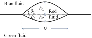
Figure 3: The shape of a liquid lens at equilibrium.

of the interfacial tensions, two different spreading phenomena can be observed, i.e. partial spreading and complete spreading.

We first consider the partial spreading, where three interfacial tensions yield a Neu-mann’s triangle. In a partial spreading, the droplet can eventually reach a steady lens shape, which is often characterized by the lens lengthDand the heightsh1andh2(see Fig. 3). The lens length and heights can be analytically given as [60, 52]

D=2 v u u u

t A

2 P

i=1 1 sinθi

_θ i

sinθi −cosθi

, (28a)

hi=

D

2

1−cosθi

sinθi

!

with i=1,2, (28b)

whereAis the area of the red droplet;θ1=ϕrgandθ2=ϕrbare the equilibrium contact

angles that can be calculated from Eq.(14). Four groups of interfacial tensions are simulated with a constantσgbof 0.01 but varyingσrbandσrg, i.e., (a)σrb=0.01 and

σrg=0.01, (b)σrb =0.0087 andσrg =0.005, (c)σrb =0.0173 andσrg =0.02, (d)

σrb=0.0058 andσrg=0.0115. The fluid viscosities are all kept at 0.1, and the final

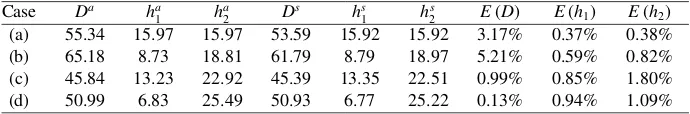
fluid distributions are shown in Fig. 4. As expected, the droplet exhibits a lens shape in each of the cases considered, and the geometrical sizes (D,h1 andh2) of the lens are case dependent. Based on the fluid distributions, we also quantify the geometrical sizes of the lens, and compare the simulated results with the analytical predictions from Eq.(28). It is seen in Table 3 that the simulated results (denoted byDs,hs₁andhs₂) agree well with the analytical predictions (denoted byDa,ha₁andha₂) with the relative errors (defined byE(χ) = |χa_χ−aχs| ×100%, where χ = D, h1 or h2) all around 1% except in the cases of small contact angles. The increased errors at small contact angles are attributed to the low resolution in sharp corners, which were also found by Jiang and Tsuji[52].

We then consider the complete spreading, where three interfacial tensions cannot yield a Neumann’s triangle. Two different cases of complete spreading are simulated forσrg=0.01 andσrg=0.015 atσgb =σrb=0.005. Clearly,σrg=σgb+σrbin the

first case, which corresponds to the critical state; whereasσrg> σgb+σrbin the second

(a) (b) (c) (d)

Figure 4: Final fluid distributions in the cases of partial spreading for (a)σrb = 0.01,σrg =0.01; (b)

σrb =0.0087,σrg =0.005; (c)σrb =0.02,σrg =0.0173; (d)σrb =0.0115,σrg =0.0058. The third

interfacial tension is fixed atσgb=0.01.

Table 3: Comparison between the analytical predictions and simulated results for the geometrical sizes of the deformed droplet.

Case Da _ha

1 h

a

2 D

s _hs

1 h

s

2 E(D) E(h1) E(h2)

(a) 55.34 15.97 15.97 53.59 15.92 15.92 3.17% 0.37% 0.38% (b) 65.18 8.73 18.81 61.79 8.79 18.97 5.21% 0.59% 0.82% (c) 45.84 13.23 22.92 45.39 13.35 22.51 0.99% 0.85% 1.80% (d) 50.99 6.83 25.49 50.93 6.77 25.22 0.13% 0.94% 1.09%

the interface in both cases for a constant fluid viscosity of 0.05. We can see that in the critical state, the red droplet sits exactly on thegbinterface in the end; whereas in the supercritical state, it bounces offthegbinterface and rises up to the blue fluid.

4. Structure and stability of double droplets

Double emulsions have received considerable attention because of their poten-tial applications in food science, cosmetics, pharmaceuticals and medical diagnostics. Since emulsion properties and functions are related to the droplet geometry and com-position, it is of great importance, from a numerical point of view, to accurately predict the topological structure of double droplets when dispersed in another immiscible fluid.

4.1. Stability diagram for double droplets

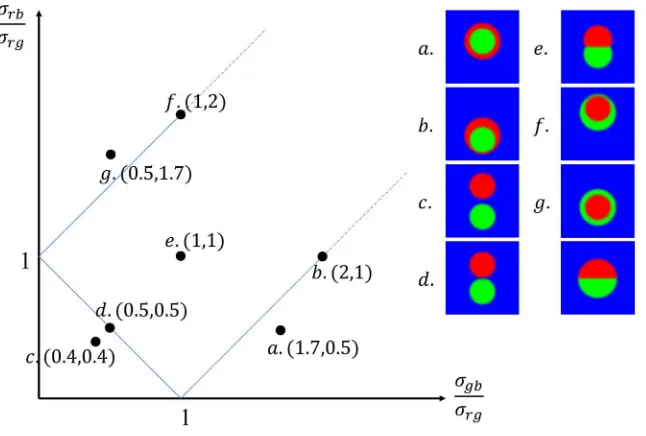
Consider a pair of equal-sized droplets, consisting of red and green fluids and ini-tially sitting next to each other, immersed in the third fluid (blue fluid). Based on the theoretical analysis, Guzowski et al.[15] presented a stability diagram that describes the possible topologies of double droplets and their transitions in terms of two ratios of the interfacial tensions (see the left panel of Fig. 6). In the stability diagram, seven typical cases (represented by the solid points) are simulated to examine if the present model is able to reproduce the correct morphologies of double droplets. These typical cases are (i) σgb

σrg = 1.7 and σrb

σrg = 0.5, (ii) σgb

σrg = 2 and σrb

σrg = 1, (iii) σgb

σrg = 0.4 and σrb

σrg = 0.4, (iv) σgb

σrg = 0.5 and σrb

σrg = 0.5, (v) σgb

σrg = 1 and σrb

σrg = 1, (vi) σgb

(a)

(b)

Figure 5: Time evolution of the interface in the cases of complete spreading for (a)σrg =0.01 and (b)

σrg=0.015. The other two interfacial tensions are fixed atσgb=σrb =0.005. Note that the system has

reached the steady state att=50000 in each case.

σrb

σrg =2, and (vii) σgb

σrg =0.5 and σrb

σrg =1.7, which cover all the possible morphologies

identified by Guzowski et al.[15].

The computational domain is taken to be [1,120]×[1,120], and the initial fluid distributions are

ρr(x,y)=0.5+0.5 tanh

"

R−

√

(x−60.5)2_+(y−60.5−R)2 ξ

#

, (29)

ρg(x,y)=0.5+0.5 tanh

"

R−

√

(x−60.5)2_{+(y−60.5+R)}2 ξ

#

, (30)

ρb(x,y)=1−ρr(x,y)−ρg(x,y), (31)

where the droplet radiusR=20 lattices. The periodic boundary conditions are used in both thexandydirections. All the fluids are assumed to have equal viscosity of 0.1, and the interfacial tensionσrgis fixed at 0.01. The simulations are run until an equilibrium

state is reached, and the equilibrium morphologies of double droplets for the seven cases are depicted in the right panel of Fig. 6. It is seen that seven different equilibrium morphologies are exhibited and they can be described as complete engulfing of green fluid by red fluid (i), critical engulfing of green fluid by red fluid (ii), separate dispersion or non-engulfing (iii), kissing (iv), partial engulfing (v), critical engulfing of red fluid by green fluid (vi), and complete engulfing of red fluid by green fluid (vii). These simulation results are consistent with the theoretical predictions by Guzowski et al.[15].

4.2. Janus droplet

Figure 6: Stability diagram representing possible morphologies of double droplets (left panel) and equi-librium shapes of the droplets for the typical cases marked in the stability diagram (right panel). The red lines represent the critical morphologies or the transitions between the regions of complete engulfing, partial engulfing and non-engulfing.

tension between the constituent fluids is negligibly small, the Janus droplet forms a perfect circle, which is known as perfect Janus droplet (PJD) [15]. Differentiating from the PJD, the Janus droplet that does not exhibit a perfect circle is called as the general Janus droplet (GJD).

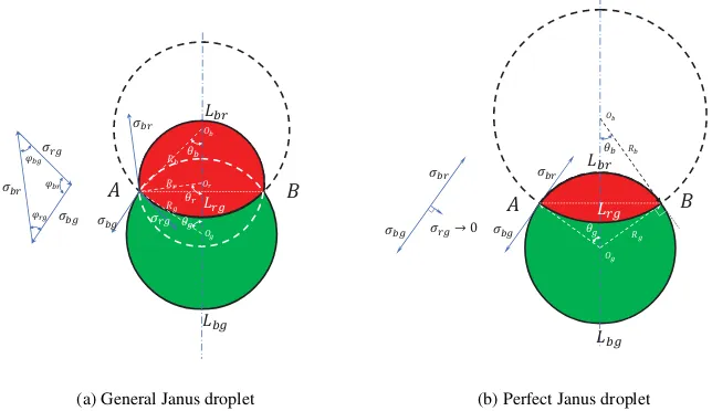
A Janus droplet, consisting of red and green fluids, is immersed in a static blue fluid. Fig. 7 shows the equilibrium geometries of a GJD and a PJD, as well as the corresponding force balances at three-phase junctions. In this figure,Rr,Rg andRb

are the curvature radii of therb,gbandrginterfaces respectively (klinterface refers to the interface between fluidkand fluidl); θr,θg andθb are the half of the central

angles subtended by the chordAB; anddrg(dgb) is the distance between the centers

Og andOr (Ob). For a GJD, provided that four independent geometric parameters,

e.g. Rr,Rg,Rbanddrg, are given, one can analytically obtain all the other geometric

parameters, includingdgb,θr,θg andθb, and the relative magnitudes ofσrb,σgb and

σrg. Specifically, the half of the central angleθgcan be first calculated by

θg=arccos

R2

g+d2rg−R2r

2Rgdrg

, (32)

which is used to calculate the other two angles,θrandθb, andRbaccording to

ܱ௕ ܱ௥ ܱ௚ ߠ௕ ߠ௥ ߠ௚ ܮ௥௚ ܮ௕௥ ܮ௕௚ ߪ௕௥

ߪ௕௚ ߪ௥௚ ܴ௚ ܴ௥ ܴ௕ ܣ ܤ ߪ௕௥ ߪ௕௚ ߪ௥௚ ߮௥௚ ߮௕௚ ߮௕௥

(a) General Janus droplet

ߪ௕௚ ߪ௕௥ ܴ௚ ܴ௕ ܱ௚ ܱ௕ ܮ௕௥ ܮ௥௚ ܮ௕௚ ߠ௕ ߠ௚ ߪ௕௚ ߪ௕௥

ߪ௥௚՜ Ͳ

ܣ ܤ

(b) Perfect Janus droplet

Figure 7: Equilibrium geometry and force balance at a three-phase junction for (a) a general Janus droplet (GJD) and (b) a perfect Janus droplet (PJD).

and the distancedgbis then obtained as

dgb =Rgcosθg+Rbcosθb. (34)

Next, we determine the anglesϕrg,ϕrbandϕgbthrough the geometric relationship and

the Neumann’s triangle shown in Fig. 7(a). For example, whenRgcosθg < dgb and

Rgcosθg≥drg, these angles can be calculated by

              

ϕrb=

π

2 −θr+θg

ϕgb=π−θr−θb

ϕrg=π−ϕrb−ϕgb

; (35)

and on the other hand, whenRgcosθg<dgbandRgcosθg <drg, we have

          

ϕrb=θb+θg

ϕgb =θr−θb

ϕrg=π−ϕrb−ϕgb

. (36)

Finally, one can obtain the relative magnitudes of the interfacial tensions by the law of Sines:

σrg

sinϕrg

= σrb

sinϕrb

= σgb

sinϕgb

. (37)

By contrast, the geometry of a PJD is only determined by two areas of the dispersed fluids, i.e.ArandAg, and its analytical solution is given by

                                

Rg=Rr=

r

Ag+Ar

π Rb=Rgtanθg

Ar

Ar+Ag

=θg−sinθgcosθg+tan

2_θ

g

_π

2−θg−sinθgcosθg

π

dgb=Rgcosθg+Rbcosθb

. (38)

The above equation suggests that one can obtain all the other geometric parameters, such asRb,θganddgb, if the area ratio _ArA₊r_Ag andRgare given.

To test the accuracy of the present model for Janus droplets, we conduct two groups of simulations with one for GJD and the other for PJD. The size of the computational domain is set as [1,300]×[1,300], and the periodic boundary conditions are used at all the boundaries. The kinematic viscosities for all the fluids are fixed atνk =0.1. In

the GJD simulations, we selectσrg=0.01,Rr =60,Rg =80 andRb =160, and vary

the distancedrgfrom 40 to 120 with an increment of 20. Using these parameters, we

can compute the geometric parametersdrganddgb as well as the interfacial tensions

σgbandσrgthrough Eqs. (32) to (37), which are presented in Table 4. We initialize the

fluid distribution such that it follows the given and analytically computed geometric parameters described above, and assume that the circles forgb,rb, andrginterfaces are initially centered at (150.5,Rg+10), (150.5,Rg+10+drg) and (150.5,Rg+10+dgb),

respectively. In the PJD simulations, we selectσrb=σgb =0.01,σrg =1×10−8and

Table 4: The interfacial tensionsσgbandσrband the distancedgbcalculated from Eqs. (32)-(37) for GJDs

withσrg=0.01,Rr=60,Rg=80 andRb=160 at different values ofdrg.

drg σgb σrb dgb

20 0.01 0.02 –

40 0.01699 0.01497 204.08

60 0.01182 0.01261 201.81

80 0.00797 0.00973 207.52

100 0.00583 0.00812 216.63

120 0.00449 0.00712 227.67

140 0.00357 0.00643 240.00

Rr = Rg = 80, and vary the area fraction _AAr

r+Ag from 0.1 to 0.5 with an increment

of 0.1. These parameters allow us to analytically compute all the other geometric parameters of a PJD, e.g. Rb anddgb, which are listed in Table 5. We follow the

analytical geometric parameters to initialize the fluid distribution, and assume that the circles forgb,rbandrginterfaces are initially located at (150.5,150.5), (150.5,150.5) and (150.5,150.5+dgb), respectively. In particular, we note that _AAr

r+Ag =0.5 leads to

Rb → ∞anddgb → ∞, suggesting that the interfacergis theoretically a straight line

Table 5: The geometric parametersRbanddgbcalculated from Eq.(38) for PJDs withRr =Rg =80 at

different area fractions.

Ar

Ar+Ag 0.1 0.2 0.3 0.4 0.5

Rb 48.32 88.39 154.12 331.92 ∞

dgb 93.46 119.22 173.64 341.43 ∞

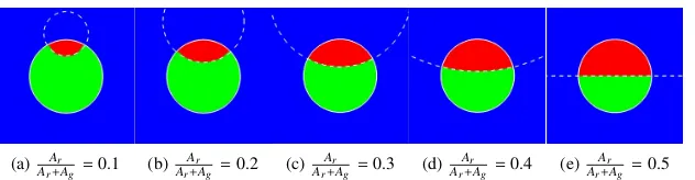
All of the simulations are run until a steady state is reached. Figs. 8 and 9 show the comparison between the analytical and simulated results for the GJDs and PJDs. In each of the figures, the analytical interface profiles are represented by the white lines of different patterns, while the red, green and blue fluids are indicated in red, green and blue, respectively. It is seen that our simulation results agree well with the analytical ones for various geometry configurations of GJD and PJD.

(a)drg=40 (b)drg=60 (c)drg=80 (d)drg=100 (e)drg=120

Figure 8: Comparison between the analytical and simulated results for GJDs withσrg =0.01,Rr =60, Rg=80 andRb=160 at different values ofdrg. The analytical interface profiles are represented by the white

lines of different patterns, while the simulated red, green and blue fluids are indicated in red, green and blue, respectively.

(a) Ar

Ar+Ag =0.1 (b)

Ar

Ar+Ag =0.2 (c)

Ar

Ar+Ag =0.3 (d)

Ar

Ar+Ag =0.4 (e)

Ar

Ar+Ag =0.5

Figure 9: Comparison between the analytical and simulated results for PJDs withRr=Rg=80 at different

area fractions. The analytical interface profiles are represented by the white lines of different patterns, while the simulated red, green and blue fluids are indicated in red, green and blue, respectively.

4.3. Near-critical and critical states

tension is close to the sum of the other two. It is challenging to accurately simulate the critical and near-critical states, where a slight inaccuracy in modeling could lead to significant simulation errors.

To highlight the strength of the present model for critical scenarios, we consider the kissing/near-kissing states and the critical/near-critical engulfing states in a rectangular domain of [1,300]×[1,300]. The boundary conditions and fluid viscosities are set the same as those in Section 4.2. In the kissing/near-kissing states, a pair of equal-sized droplets with the radii ofRr = Rg = 60 are initially placed with a distance of drg,

and they are symmetric with respect to the centerliney=150.5. The simulations are performed for a constantσrgof 0.01 but varyingσgb (=σrb), which is varied around

the critical value of 0.005 with an increment of 2×10−4_{. Note that the initial distance}

drgdepends on the value ofσgb, and is given by its analytical value in equilibrium as

drg=

    

Rrσrg/σgb ifσgb>0.005;

Rr+Rg=120 otherwise.

(39)

In the critical/near-critical engulfing states, we consider a green droplet withRg =

80 entirely or partially engulfing a red droplet withRr=60 forσgb =σrg=0.01.σrb

is varied around the critical value of 0.02 with an increment of 2×10−4. With these parameters, we are able to analytically compute other geometric parameters, which are given bydrg =

q

R2

r+R2g−2RrRgcosα,Rb = Rgsinθg

sinθb anddgb =Rgcosθg−Rbcosθb

forσrb < 0.02, and bydrg = Rg −Rr = 20 forσrb ≥ 0.02. Herein, cosα = _2σσrb_gb,

θg =arccos R2

g+dgr2−R2r

2Rgdgr andθb =θg+2α. Again, we initialize the fluid distribution such

that it follows the analytical geometric parameters.

Vgb

Lrg

0.004 0.0045 0.005 0.0055 0.006 -20

0 20 40 60 80

Theory The present model The model of Fu et al. The model of Leclaire et al.

The exact kissing state

(a)

Vrb

Lrb

0.019 0.0195 0.02 0.0205 0.021 0

50 100 150 200

250 Theory

The present model The model of Fu et al. The model of Leclaire et al.

The critical engulfing state

(b)

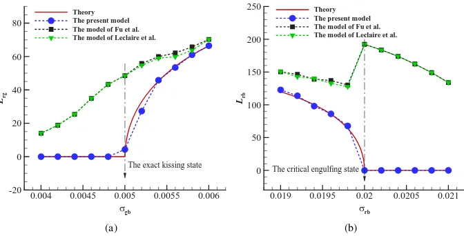
Figure 10: (a) The interface lengthLrgas a function ofσgbin the kissing/near-kissing states; (b) the interface

lengthLrbas a function ofσrbin the critical/near-critical engulfing states.

state, we quantify the interface lengthsLrgin the kissing/near-kissing states andLrbin

the critical/near-critical engulfing states. Fig. 10 compares the simulated results from the present model with those from the model of Fu et al.[51] and the model of Leclaire et al.[50], and the analytical solutions. It is seen that for either kissing/near-kissing states or critical/near-critical engulfing states, the simulated results from the present model are in good agreement with the analytical solutions, while the simulated results from the other two models significantly deviate from the analytical solutions. Fig. 11 shows the final fluid distributions obtained by the present model and the model of Fu et al.[51], in both kissing and critical engulfing states. Note that the fluid distribution from the model of Leclaire et al.[50] is not shown in the figure, since it produces almost the same results as the model of Fu et al.[51]. Clearly, both critical states are correctly reproduced by the present model but not by the model of Fu et al.[51]. These results indicate that the present model is advantageous to simulate critical state in ternary fluids.

(a) (b) (c) (d)

Figure 11: The final fluid distributions obtained by (a) the present model and (b) the model of Fu et al. [51] for the kissing state, and by (c) the present model and (d) the model of Fu et al. [51] for the critical engulfing state.

5. conclusions

A LB color-gradient model is proposed to simulate immiscible ternary fluids with a full range of interfacial tensions. An interfacial force formulation forN-phase (N≥3) systems is derived and then introduced into the model using a body force scheme, which is found to effectively reduce spurious velocities. A recoloring algorithm pro-posed by Spencer et al.[49] is applied to produce the phase segregation and ensure the immiscibility of three different fluids, where a novel form of segregation parame-ters is proposed by considering the existence of Neumann’s triangle and the effect of equilibrium contact angle in three-phase junction. The model’s capability in capturing interfaces and modeling interfacial tensions is first validated by the simulation of the two separate static droplets and the Young-Laplace test for a compound droplet. The overall performance of the model is then assessed by simulating the spreading of a droplet between two stratified fluids, and both the partial and complete spreadings are predicted with satisfactory accuracy.

ratios of the interfacial tensions, seven possible equilibrium morphologies are success-fully reproduced, which are consistent with the theoretical stability diagram by Gu-zowski et al.[15]. For various geometry configurations of general and perfect Janus droplets, good agreemento between simulated results and analytical solutions shows the present model is accurate when three interfacial tensions yield a Neumann’s trian-gle. In addition, we also simulate the near-critical and critical states of double droplets, which is challenging since the outcomes are very sensitive to the model accuracy. It is found that the simulated results from the present model agree well with the ana-lytical solutions, while the simulated results from the existing color-gradient models significantly deviate from the analytical solutions, especially in critical states. In sum-mary, the present work provides the first LB multiphase model that allows for accurate simulation of ternary fluid flows with a full range of interfacial tensions.

Acknowledgements

This work was supported by the National Natural Science Foundation of China (Nos. 51506168, 51711530130), the National Key Research and Development Project of China (No. 2016YFB0200902), the China Postdoctoral Science Foundation (No. 2016M590943), Guangdong Provincial Key Laboratory of Fire Science and Technol-ogy (No. 2010A060801010) and Guangdong Provincial Scientific and Technological Project (No. 2011B090400518). Y. Yu was supported by the China Scholarship Coun-cil for one year study at the University of Strathclyde, UK. H. Liu gratefully acknowl-edges the financial supports from Thousand Youth Talents Program for Distinguished Young Scholars, the Young Talent Support Plan of Xi’an Jiaotong University.

References

[1] A. S. Utada, E. Lorenceau, D. R. Link, P. D. Kaplan, H. A. Stone, D. A. Weitz, Monodisperse double emulsions generated from a microcapillary device, Science 308 (2005) 537–541.

[2] N. Bhatia, S. Pandit, S. Agrawal, D. Gupta, A review on multiple emulsions, International Journal of Pharmaceutical Erudition 3 (2013) 22–30.

[3] H. Lamba, K. Sathish, L. Sabikhi, Double emulsions: Emerging delivery system for plant bioactives, Food and Bioprocess Technology 8 (2015) 709–728. [4] D. Chong, X. Liu, H. Ma, G. Huang, Y. L. Han, X. Cui, J. Yan, F. Xu,

Ad-vances in fabricating double-emulsion droplets and their biomedical applications, Microfluidics and Nanofluidics 19 (2015) 1071–1090.

[5] M. A. Augustin, Y. Hemar, Nano- and micro-structured assemblies for encapsu-lation of food ingredients, Chemical Society Reviews 38 (2009) 902–912. [6] V. B. Patravale, S. D. Mandawgade, Novel cosmetic delivery systems: an

[7] E. E. Ekanem, S. A. Nabavi, G. T. Vladisavljevi, S. Gu, Structured biodegrad-able polymeric microparticles for drug delivery produced using flow focusing glass microfluidic devices, ACS Applied Materials & Interfaces 7 (2015) 23132– 23143.

[8] B. Ahmed, D. A. Barrow, T. Wirth, Enhancement of reaction rates by segmented fluid flow in capillary scale reactors, Advanced Synthesis & Catalysis 348 (2006) 1043–1048.

[9] L. Chen, Y. Li, J. Fan, H. K. Bisoyi, D. A. Weitz, Q. Li, Microshells: Pho-toresponsive monodisperse cholesteric liquid crystalline microshells for tunable omnidirectional lasing enabled by a visible lightdriven chiral molecular switch (advanced optical materials 9/2014), Advanced Optical Materials 2 (2014) 904– 904.

[10] K. Funakoshi, H. Suzuki, S. Takeuchi, Lipid bilayer formation by contacting monolayers in a microfluidic device for membrane protein analysis, Analytical chemistry 78 (2006) 8169–8174.

[11] P. G. De Gennes, Soft matter, Reviews of Modern Physics 64 (1992) 645–648. [12] G. Vladisavljevi, R. A. Nuumani, S. Nabavi, Microfluidic production of multiple

emulsions, Micromachines 8 (2017) 75.

[13] S. Torza, S. Mason, Coalescence of two immiscible liquid drops, Science 163 (1969) 813–814.

[14] N. Pannacci, H. Bruus, D. Bartolo, I. Etchart, T. Lockhart, Y. Hennequin, H. Willaime, P. Tabeling, Equilibrium and nonequilibrium states in microfluidic double emulsions, Physical review letters 101 (2008) 164502.

[15] J. Guzowski, P. M. Korczyk, S. Jakiela, P. Garstecki, The structure and stability of multiple micro-droplets, Soft Matter 8 (2012) 7269–7278.

[16] M. Muradoglu, S. Tasoglu, A front-tracking method for computational modeling of impact and spreading of viscous droplets on solid walls, Computers & Fluids 39 (2010) 615–625.

[17] R. Bonhomme, J. Magnaudet, F. Duval, B. Piar, Inertial dynamics of air bubbles crossing a horizontal fluid–fluid interface, Journal of Fluid Mechanics 707 (2012) 405–443.

[18] H.-K. Zhao, T. Chan, B. Merriman, S. Osher, A variational level set approach to multiphase motion, Journal of computational physics 127 (1996) 179–195. [19] K. A. Smith, F. J. Solis, D. Chopp, A projection method for motion of triple

junctions by level sets, Interfaces and free boundaries 4 (2002) 263–276. [20] R. I. Saye, J. A. Sethian, The voronoi implicit interface method for computing

[21] F. Boyer, C. Lapuerta, Study of a three component cahn-hilliard flow model, Mathematical Modelling and Numerical Analysis 40 (2006) 653–687.

[22] F. Boyer, C. Lapuerta, S. Minjeaud, B. Piar, M. Quintard, Cahn-hilliard/ navier-stokes model for the simulation of three-phase flows, Transport in Porous Media 82 (2010) 463–483.

[23] J. Kim, J. S. Lowengrub, Phase field modeling and simulation of three-phase flows, Interfaces and Free Boundaries 7 (2005) 435–466.

[24] J. Kim, Phase field computations for ternary fluid flows, Computer Methods in Applied Mechanics and Engineering 196 (2007) 4779–4788.

[25] J. Kim, A generalized continuous surface tension force formulation for phase-field models for multi-component immiscible fluid flows, Computer Methods in Applied Mechanics and Engineering 198 (2009) 3105–3112.

[26] J. Kim, Phase-field models for multi-component fluid flows, Communications in Computational Physics 12 (2012) 613–661.

[27] H. Liu, Y. Ba, L. Wu, Z. Li, G. Xi, Y. Zhang, A hybrid lattice boltzmann and finite difference method for droplet dynamics with insoluble surfactants, Journal of Fluid Mechanics 837 (2018) 381–412.

[28] H. Liu, A. J. Valocchi, Q. Kang, Three-dimensional lattice boltzmann model for immiscible two-phase flow simulations, Physical Review E 85 (2012) 046309. [29] X. He, L.-S. Luo, A priori derivation of the lattice boltzmann equation, Physical

Review E 55 (1997) R6333.

[30] S. Chen, G. D. Doolen, Lattice boltzmann method for fluid flows, Annual review of fluid mechanics 30 (1998) 329–364.

[31] C. K. Aidun, J. R. Clausen, Lattice-boltzmann method for complex flows, Annual review of fluid mechanics 42 (2010) 439–472.

[32] A. K. Gunstensen, D. H. Rothman, S. Zaleski, G. Zanetti, Lattice boltzmann model of immiscible fluids., Physical Review A 43 (1991) 4320–4327.

[33] T. Reis, T. N. Phillips, Lattice boltzmann model for simulating immiscible two-phase flows, Journal of Physics A 40 (2007) 4033–4053.

[34] X. Shan, H. Chen, Lattice boltzmann model for simulating flows with multiple phases and components, Physical Review E Statistical Physics Plasmas Fluids & Related Interdisciplinary Topics 47 (1993) 1815.

[35] X. Shan, H. Chen, Simulation of nonideal gases and liquid-gas phase transitions by the lattice boltzmann equation, Physical Review E 49 (1994) 2941–2948. [36] M. Sbragaglia, R. Benzi, L. Biferale, S. Succi, K. Sugiyama, F. Toschi,

[37] M. Sbragaglia, R. Benzi, M. Bernaschi, S. Succi, The emergence of supramolec-ular forces from lattice kinetic models of non-ideal fluids: applications to the rheology of soft glassy materials, Soft Matter 8 (2012) 10773–10782.

[38] B. Dollet, A. Scagliarini, M. Sbragaglia, Two-dimensional plastic flow of foams and emulsions in a channel: experiments and lattice boltzmann simulations, Jour-nal of Fluid Mechanics 766 (2015) 556–589.

[39] M. R. Swift, E. Orlandini, W. Osborn, J. Yeomans, Lattice boltzmann simulations of liquid-gas and binary fluid systems, Physical Review E 54 (1996) 5041. [40] Y. Wang, C. Shu, H. Huang, C. Teo, Multiphase lattice boltzmann flux solver for

incompressible multiphase flows with large density ratio, Journal of Computa-tional Physics 280 (2015) 404–423.

[41] Y. Wang, C. Shu, L. M. Yang, An improved multiphase lattice boltzmann flux solver for three-dimensional flows with large density ratio and high reynolds num-ber, Journal of Computational Physics 302 (2015) 41–58.

[42] X. He, S. Chen, R. Zhang, A lattice boltzmann scheme for incompressible multi-phase flow and its application in simulation of rayleigh-taylor instability, Journal of Computational Physics 152 (1999) 642–663.

[43] H. Chen, B. M. Boghosian, P. V. Coveney, A ternary lattice boltzmann model for amphiphilic fluids, Proceedings of The Royal Society A: Mathematical, Physical and Engineering Sciences 456 (2000) 2043–2057.

[44] O. Shardt, J. J. Derksen, S. K. Mitra, Simulations of janus droplets at equilibrium and in shear, Physics of Fluids 26 (2014) 106–114.

[45] H. Liang, B. C. Shi, Z. Chai, Lattice boltzmann modeling of three-phase incom-pressible flows., Physical Review E 93 (2016) 013308.

[46] C. Semprebon, T. Kruger, H. Kusumaatmaja, Ternary free energy lattice boltz-mann model with tunable surface tensions and contact angles, Physical Review E 93 (2016) 033305.

[47] M. W¨ohrwag, C. Semprebon, A. M. Moqaddam, I. Karlin, H. Kusumaatmaja, Ternary free-energy entropic lattice boltzmann model with high density ratio, arXiv preprint arXiv:1710.07486 (2017).

[48] Y. Shi, G. Tang, Y. Wang, Simulation of three-component fluid flows using the multiphase lattice boltzmann flux solver, Journal of Computational Physics 314 (2016) 228–243.

[49] T. Spencer, I. Halliday, C. M. Care, Lattice boltzmann equation method for mul-tiple immiscible continuum fluids, Physical Review E 82 (2010) 066701. [50] S. Leclaire, M. Reggio, J. Trepanier, Progress and investigation on lattice

[51] Y. Fu, S. Zhao, L. Bai, Y. Jin, Y. Cheng, Numerical study of double emulsion formation in microchannels by a ternary lattice boltzmann method, Chemical Engineering Science 146 (2016) 126–134.

[52] F. Jiang, T. Tsuji, Estimation of threephase relative permeability by simulating fluid dynamics directly on rockmicrostructure images, Water Resources Research 53 (2017) 11–32.

[53] H. Liu, Y. Zhang, Modelling thermocapillary migration of a microfluidic droplet on a solid surface, Journal of Computational Physics 280 (2015) 37–53.

[54] Z. Guo, C. Zheng, B. Shi, Discrete lattice effects on the forcing term in the lattice boltzmann method., Physical Review E 65 (2002) 046308.

[55] I. Halliday, C. M. Care, A. P. Hollis, Improved simulation of drop dynamics in a shear flow at low reynolds and capillary number, Physical Review E 73 (2006) 056708.

[56] U. d’Ortona, D. Salin, M. Cieplak, R. B. Rybka, J. R. Banavar, Two-color nonlin-ear boltzmann cellular automata: surface tension and wetting, Physical Review E 51 (1995) 3718.

[57] M. Latva-Kokko, D. H. Rothman, Diffusion properties of gradient-based lattice boltzmann models of immiscible fluids, Physical Review E 71 (2005) 056702. [58] H. Liu, L. Wu, Y. Ba, G. Xi, A lattice boltzmann method for axisymmetric

ther-mocapillary flows, International Journal of Heat and Mass Transfer 104 (2017) 337–350.

[59] A. Riaud, S. Zhao, K. Wang, Y. Cheng, G. Luo, Lattice-boltzmann method for the simulation of multiphase mass transfer and reaction of dilute species, Physical Review E 89 (2014) 053308.