Vol. 40, No. 1, pp. 320–346 of the Creative Commons 4.0 license
MAX-BALANCED HUNGARIAN SCALINGS∗
JAMES HOOK†, JENNIFER PESTANA‡, FRANC¸ OISE TISSEUR§, AND JONATHAN HOGG¶
Abstract. A Hungarian scaling is a diagonal scaling of a matrix that is typically applied along with a permutation to a sparse linear system before calling a direct or iterative solver. A matrix that has been Hungarian scaled and reordered has all entries of modulus less than or equal to 1 and entries of modulus 1 on the diagonal. An important fact that has been largely overlooked by the previous research into Hungarian scaling of linear systems is that a given matrix typically has a range of pos-sible Hungarian scalings, and direct or iterative solvers may behave quite differently under each of these scalings. Since standard algorithms for computing Hungarian scalings return only one scaling, it is natural to ask whether a superior performing scaling can be obtained by searching within the set of all possible Hungarian scalings. To this end we propose a method for computing a Hungarian scaling that is optimal from the point of view of a measure of diagonal dominance. Our method uses max-balancing, which minimizes the largest off-diagonal entries in the scaled and permuted matrix. Numerical experiments illustrate the increased diagonal dominance produced by max-balanced Hun-garian scaling as well as the reduced need for row interchanges in Gaussian elimination with partial pivoting and the improved stability of LU factorizations without pivoting. We additionally find that applying the max-balancing scaling before computing incomplete LU preconditioners improves the convergence rate of certain iterative methods. Our numerical experiments also show that the Hun-garian scaling returned by the HSL code MC64 has performance very close to that of the optimal max-balanced Hungarian scaling, which further supports the use of this code in practice.
Key words. max-plus algebra, diagonal scaling, Hungarian scaling, max-balancing, diagonal dominance, linear systems of equations, sparse matrices, incomplete LU preconditioner
AMS subject classifications. 65F35, 15A12, 15A60, 15A80 DOI. 10.1137/15M1024871
1. Introduction. A Hungarian scaling is a two-sided diagonal scaling of a ma-trix that is applied along with a permutation P to a linear system Ax = b, with A∈Cn×n andb∈Cn, yielding
(1.1) H =P D1AD2, Hy=P D1b, x=D2y,
whereD1, D2∈Rn×nare diagonal and nonsingular. The scaled and reordered matrix H = (hij) is such that |hij| ≤ 1 and |hii| = 1 for i, j = 1, . . . , n. A permutation
matrix P, such that (1.1) holds, is commonly referred to as an optimal assignment forA.
Olschowka and Neumaier [16] propose applying a Hungarian scaling together with a permutation to matrices prior to performing Gaussian elimination. They prove that
∗Received by the editors June 8, 2015; accepted for publication (in revised form) December 19, 2018; published electronically February 26, 2019.
http://www.siam.org/journals/simax/40-1/M102487.html
Funding: The work of the first, second, and third authors was supported by Engineering and Physical Sciences Research Council grant EP/I005293. The work of the third author was also sup-ported by a Royal Society-Wolfson Research Merit Award.
†Department of Mathematical Sciences, University of Bath, Bath, BA2 7AY, UK ([email protected]).
‡Department of Mathematics and Statistics, University of Strathclyde, Glasgow, G1 1XH, UK ([email protected]).
§School of Mathematics, The University of Manchester, Manchester, M13 9PL, UK ([email protected]).
¶Scientific Computing Department, STFC Rutherford Appleton Laboratory, Harwell, Oxford, Didcot, OX11 0QX, UK ([email protected]).
320
this preprocessing step eliminates the need for row interchanges for some special class of matrices. Some intuitive explanation for this widely observed fact is provided in Hook and Tisseur [13, Thm. 3.9] for general matrices. Duff and Koster [7, 8] describe an efficient algorithm for computing a Hungarian scaling, on which the HSL code MC64 is based [14]. They show that applying the scaling and permutation significantly reduces the number of delayed pivots during factorization of sparse nonsymmetric matrices by a multifrontal direct solver [8]. The authors explain this phenomenon by pointing out that the Hungarian scaled matrix H tends to be more diagonally dominant than the original matrixA.
Benzi, Haws, and T˚uma [1] show that Hungarian scaling is an effective prepro-cessing step before applying BiCGSTAB, GMRES, or TFQMR to sparse indefinite nonsymmetric matrices. The scaled matrices require significantly fewer iterations for convergence. Again, the authors explain this phenomenon by pointing out that the Hungarian scaled matrixH in (1.1) tends to be more diagonally dominant than the original matrix A. The authors also experiment with using Hungarian scaling as a preprocessing step before applying preconditioned BiCGSTAB with an incomplete LU (ILU) preconditioner. Without scaling they show that there are many problems for which attempts to compute a very sparse ILU preconditioner break down. In these cases, to reliably compute effective ILU preconditioners they are forced to compute denser ILU factors at a considerably increased cost. However, they show that after Hungarian scaling has been applied it is possible to reliably compute very sparse ILU preconditioners.
In the symmetric case, rather than permuting matched entries (unsymmetrically) to the main diagonal, these entries can instead be permuted (symmetrically) to the subdiagonal and used in 2×2 block pivots. However, in the sparse case, doing so conflicts with the minimization of fill-in. Various compromises have been proposed. In [11] and [12] Hogg and Scott show that for most matrices merely using the sym-metrized Hungarian scaling is sufficient to eliminate the need for significant amounts of pivoting in LDLT factorizations with threshold partial pivoting. For the class of
problems where this is not the case, reordering roughly half the matched entries onto the subdiagonal and then applying a constrained fill-reducing ordering is sufficient to reduce pivoting to a manageable level.
Olschowka and Neumaier [16, Alg. 4.2] describe a second round of scaling with a nonsingular diagonal matrix S applied to the Hungarian scaled matrixH in (1.1). When the optimal assignment permutation is unique, this second round of scaling yields the doubly scaled matrixS−1HSwith all off-diagonal entries of modulus strictly less than one [16, Thm. 4.3]. This is equivalent to choosing a different pair of diag-onal matrices D1, D2 in the initial Hungarian scaling (1.1). However, the fact that the Hungarian scaling and reordering associated with a matrix A ∈ Cn×n are not necessarily unique has been overlooked in subsequent research into Hungarian scaling of linear systems, and there have not been any numerical experiments that compare the effectiveness of different Hungarian scalings. In general there is a range of dif-ferent diagonal matrix pairs D1, D2 ∈ Rn×n and permutation matrices P ∈ Rn×n which results in different Hungarian scaled and reordered matrices, for which direct or iterative solvers may behave quite differently. Since the increased diagonal domi-nance of the Hungarian scaled matrices has been repeatedly cited as responsible for their improved numerical characteristics, we focus in this paper on trying to obtain Hungarian scaled matrices that are as diagonally dominant as possible. For this, we
consider row-wise diagonal dominance measures of the form
(1.2) ∆(A) =g
p s
P
j6=i|aij|p
|aii|p !
i=1,...,n
for somep∈[1,∞) and whereg :Rn+ 7→R+ is some function that amalgamates the individual rowp-norm scores into a single score for the whole matrix.
While the choice of optimal assignment permutation may impact the number of row interchanges required during Gaussian elimination, it is difficult to predict which permutations will work best in advance. Although the choice of optimal assignment permutation might affect the diagonal dominance of a general matrix, we will show that once a matrix has been Hungarian scaled, all of the possible choices of optimal assignment permutation result in scaled and reordered matrices with the same measure of diagonal dominance. Hence we focus on the choice of diagonal matrices D1 and D2 defining the Hungarian scaling and, in particular, on the following two questions: What does the set of all Hungarian scalings of a matrix look like? And how do we choose the best possible Hungarian scaling for a particular problem?
To answer these questions we will use results from max-plus algebra, to which we give a brief introduction in section 2. It turns out that the different Hungarian scalings of a matrixAare all related by diagonal similarities, so that ifH =P D1AD2 and H0 =P D01AD02 are both Hungarian scaled, then there exists a diagonal matrix S such thatH0 =S−1HS. Therefore, starting from one Hungarian scaling, we can generate new Hungarian scalings by applying “special” diagonal similarities. The diagonal matrixS must be such thatH0 retains the properties of a Hungarian scaled matrix, i.e.,|h0
ij| ≤1 and|h0ii|= 1 for alli, j. These conditions onSare very naturally
expressed in terms of max-plus algebra, and that is why it proves so useful here; see Theorem 2.5.
In order to compute a Hungarian scaling that is as diagonally dominant as possi-ble, we use a technique called max-balancing. Max-balanced graphs were introduced by Schneider and Schneider in connection with certain network flow problems [20]. A directed weighted graph is max-balanced if for any subset of vertices the maximum weight of an edge into that subset is equal to the maximum weight of an edge out of that subset. We can use the max-balancing algorithm of Schneider and Schneider to compute a nonsingular diagonal matrix S ∈ Rn×n such that the scaled matrix M = S−1HS is max-balanced. Intuitively, max-balancing is the similarity scaling obtained by first minimizing the largest off-diagonal entry in the matrix, then mini-mizing the next largest entry subject to minimini-mizing the first, and so on.
We show in section 3 that max-balancing (a) preserves the property of a matrix being Hungarian scaled and (b) minimizes the entrywise p-norm over all diagonal similarity scalings of A in the limit as p tends to infinity; see Theorem 3.2. As a result, the max-balancing of a Hungarian scaled matrix tends to be more diagonally dominant than the initial Hungarian scaling H. Theorem 3.8, which is the main theoretical result of this paper, states that the max-balanced Hungarian scaling ofA is the unique optimal scaling and reordering ofAwith respect to a particularp-norm diagonal dominance measure in the limit asptends to infinity. If we were to attempt to minimize some other measure of diagonal dominance via similarity scaling, then there would be no guarantee that we would be able to preserve the properties of being Hungarian scaled, i.e., that no off-diagonal entries have modulus greater than 1. The elegance of the max-balanced Hungarian scaling is that both diagonal dominance and Hungarian scaling are achieved simultaneously.
To demonstrate the effectiveness of max-balancing we include numerical experi-ments in section 4. We focus on solvingAx=bvia LU factorization, whereA∈Cn×n is sparse and nonsymmetric. Our experiments confirm that max-balancing improves diagonal dominance. Additionally, the condition number and number of row inter-changes in Gaussian elimination with partial pivoting, reduced by Hungarian scaling, are further reduced by balancing Hungarian scaling. Finally, we apply the max-balancing scaling before computing incomplete LU preconditioners for GMRES and BiCGStab and find that doing so reduces the number of iterations for both methods.
2. Introduction to max-plus algebra and Hungarian scaling. We intro-duce in this section the basic max-plus algebra concepts that are needed to understand the theoretical results in our paper. Max-plus algebra concerns the max-plus semiring Rmax=R∪ {−∞}, which is equipped with the binary operations max and plus,
a
⊕b
= max{a
,b
},a
⊗b
=a
+b
for alla
,b
∈Rmax,with−∞and 0 playing the role of additive and multiplicative identities. Throughout this paper we use calligraphic letters for elements of Rmax. A max-plus matrixA ∈ Rnmax×mis simply an array of elements fromRmax.
Max-plus matrix multiplication is defined analogously to classical matrix multi-plication so that ifA ∈Rnmax×mandB ∈Rmaxm×`, thenA ⊗ B ∈Rnmax×` with
A ⊗ B ij =
m M
k=1
aik
⊗bkj
= max1≤k≤m
aik
+bkj
.A max-plus diagonal matrix has all off-diagonal entries equal to minus infinity. Let diag∞(d) denote the max-plus diagonal matrix with diagonal entries given by some vector d ∈ Rnmax; we use the subscript ∞ to distinguish them from classical n×n complex diagonal matrices, which we denote by diag(b) for some b ∈ Cn. For A ∈
Rnmax×n and foru, v∈Rn, we have
diag∞(−u)⊗ A ⊗diag∞(−v)
ij=
aij
−ui−vj.Themax-plus permanent ofA ∈Rnmax×n is given by
(2.1) perm(A) = max
π∈Π(n)
n X
j=1
aπ
(j)j,where the maximum is taken over the set Π(n) of all permutations of{1, . . . , n}. We denote by π = id the identity permutation, i.e., id = {1, . . . , n}. A permutationπ which attains the maximum in (2.1) is called an optimal assignment of A. When perm(A) 6=−∞, the max-plus permanent ofA can be rewritten as a minimization problem,
(2.2) perm(A) = min
n X
i=1
(ui+vi) : u, v ∈Rn,
a
ij−ui−vj≤0.
A Hungarian pair of A is an optimal solution (u, v) to (2.2). It is named after the Hungarian algorithm, which is a widely used primal-dual algorithm for solving the optimal assignment problem.
Forπ∈Π(n) denote byPπ then×nclassical permutation and byPπ then×n
max-plus permutation matrix, both defined by
(2.3) (Pπ)ij =
1 forj=π(i),
0 otherwise, (Pπ)ij=
0 forj=π(i), −∞ otherwise.
The following theorem, or, more precisely, its corollary for complex matrices, appears in [16, Thm. 2.8].
Theorem 2.1 (Hungarian scaling). ForA ∈Rnmax×n, withperm(A)6=−∞, letπ
and(u, v)be an optimal assignment and Hungarian pair ofA, respectively. Then the max-plus Hungarian scaled and reordered matrix
H=Pπ⊗diag∞(−u)⊗ A ⊗diag∞(−v)
is such that
h
ij≤0 andh
ii = 0for all i, j= 1, . . . , n.To link the classical algebra of complex matrices with standard addition and multiplication to the max-plus algebra, we use the following transformation, which is known as a non-Archimedean valuation:
(2.4) V :C7→Rmax, V(x) = log|x|,
with the convention that log 0 = −∞. For matrices, we apply the valuation com-ponentwise; that is, for A ∈ Cn×n, V(A) = A = log|aij|
∈ Rnmax×n. Note that perm(A) 6= −∞ with A = V(A) means that A is not structurally rank deficient. The next result, which holds for complex or real matrices, is a direct consequence of Theorem 2.1.
Corollary 2.2. LetA∈Cn×n be of full structural rank. Letπand(u, v)be an
optimal assignment and a Hungarian pair ofV(A), respectively. Then the Hungarian scaled and reordered matrix
(2.5) H =Pπdiag exp(−u)
Adiag exp(−v)
is such that |hij| ≤1 and|hii|= 1 for alli, j= 1, . . . , n.
We note that the max-plus matrix Hin Theorem 2.1 is the componentwise log-of-absolute-value of the matrixH in Corollary 2.2, that is,H=V(H).
The max-plus matrixA=V(A) may have more than one optimal assignment and the optimal solution (u, v) to (2.2) is in general not unique. Let us look at a simple example to illustrate the latter point.
Example 2.3. Let A∈R3×3 andA:=V(A)∈R3×3max be given by
A=
exp(6) exp(6) exp(9)
exp(−4) exp(−3) exp(−2)
0 exp(−7) 1
, A=
6 6 9
−4 −3 −2
−∞ −7 0
.
It is easy to check that the max-plus matrix Ahas a unique optimal assignmentπ= (1,2,3) and that (u, v) with u= [0,−9,−9]T andv = [6,6,9]T is a Hungarian pair
forAyielding the Hungarian scaled matrix
(2.6) H = diag exp(−u)
Adiag exp(−v)
=
1 1 1
exp(−1) 1 exp(−2)
0 exp(−4) 1
.
Hungarian scaling tends to significantly reduce the matrix 2-norm condition number
κ2(A) =kAk2kA−1k2. For this example we haveκ2(A) = 4.1×10⁵ κ2(H) = 6.2.
Note also thatH is more diagonally dominant thanA.
We will show in the next section that if (us, vs) is another Hungarian pair for
A, then there exists s∈R3 such that(us, vs) = (u+s, v−s). This means that the
Hungarian scaled matrices
Hs= diag exp(−us)
Adiag exp(−vs)
= diag exp(−s)
Hdiag exp(s)
and H are similar. But not all diagonal similarity scalings of H are Hungarian scalings ofA: the vector smust be such that Hs is a Hungarian matrix. Indeed, Hs
is Hungarian if and only if|(Hs)ij| ≤1 for alli, j= 1,2,3. This yields the following
constraints on the entries ofs:
(2.7) −1 +s1−s2≤0, s2−s1≤0, −4 +s2−s3≤0, s3−s1≤0.
Now for all α ∈R, s∈ R3 satisfies (2.7) if and only if ˜s:=s+α[1,1,1]T satisfies (2.7). Therefore, the set S(H) := {s ∈ R3 : Hs is Hungarian} is a prism extruded
in the [1,1,1]T direction. It is not difficult to see that for any α∈ R, s and s˜give
rise to the same scaling ofH, so there is no loss of generality in choosingαsuch that
s1= 0. Then the intersection ofS(H)with the planes1= 0 is the set of solutions to
s2≥ −1, s2≤0, s2−s3≤4, s3≤0,
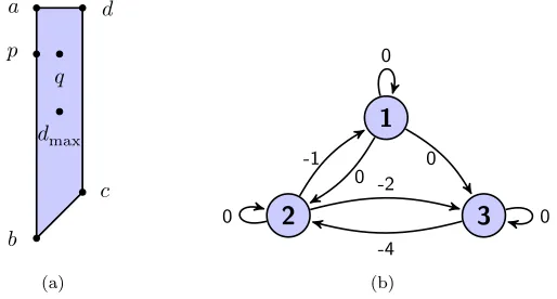
which is given by the quadrilateral shown in Figure 2.1(a). The vertices a, b, c, d of the quadrilateral are are given by
a= [0,−1,0]T, b= [0,−1,−5]T, c= [0,0,−4]T, d= [0,0,0]T.
They correspond to extremal Hungarian scalings ofA given by
Ha =
1 exp(−1) 1
1 1 exp(−1)
0 exp(−5) 1
, Hb=
1 exp(−1) exp(−5)
1 1 exp(−6)
0 1 1
,
Hc=
1 1 exp(−4)
exp(−1) 1 exp(−6)
0 1 1
, Hd=
1 1 1
exp(−1) 1 exp(−2)
0 exp(−4) 1
.
Each of these Hungarian scaled matrices contain precisely five entries equal to one. If we scale using any parameter from the relative interior of an edge of the quadrilateral, then we obtain a scaled matrix with exactly four entries equal to one. At the end of section 2.2 we will see that if we take any scaling parameter from the interior of this quadrilateral, then we obtain a scaled matrix with exactly three entries equal to one. For example, p= [0,−1,−1]T andq= [0,−0.5,−1]T yield
Hp =
1 exp(−1) exp(−1)
1 1 exp(−2)
0 exp(−4) 1
, Hq =
1 exp(−1
2) exp(−1) exp(−1
2) 1 exp(−
5 2)
0 −exp(72) 1
.
The2-norm and2-norm condition number of these matrices are provided in Table2.1. The scalings a, b, c, d which are taken from extreme points of the quadrilateral all result in scaled matrices with very similar condition numbers and norms. The scaling
a
b
c d
p q
dmax
(a)
1
2
3
0 0
0
-1
0
-2
-4
0
(b)
Fig. 2.1. (a)shows S(H)∩ {s1= 0} for the matrixH ∈R3×3 of Example 2.3 and different
[image:7.612.129.386.104.242.2]scaling vectors;(b)shows the precedence graphΓ(H)forH=V(H).
Table 2.1
Frobenius norm and2-norm condition number for the matrices of Examples 2.3and 3.11(for
Hdmax).
MatrixX A H(=Hd) Ha Hb Hc Hp Hq Hdmax kXkF 8.12e3 2.27 2.30 2.27 2.27 2.07 1.97 1.94 κ2(X) 4.14e5 6.19 6.56 6.98 6.40 4.96 4.27 4.08
p taken from an edge of the quadrilateral results in a scaled matrix with a slightly smaller condition number and norm compared to the previous Hungarian scalings. The scaling q taken from the interior of the quadrilateral results in a scaled matrix that has a further reduced condition number and norm.
We show in Theorem 2.5 that the set of all Hungarian pairs of a matrix, in this example the extruded quadrilateral S(H), is actually given by the column space of a related max-plus matrix. We also show how max-balancing provides a way to automatically select a vector from the middle of the interior of this set. Just as max-plus algebra provides a neat characterization of the set of Hungarian all pairs, it also provides the perfect framework to describe the max-balancing algorithm and prove results about the properties of max-balanced scaled matrices, as we shall see. In Table 2.1 the max-balancing scaling vector dmax, which we show how to calculate in Example 3.11, performs the best at reducing the norm and condition number. We explain this performance from the improved diagonal dominance brought about by max-balancing. Theorem 3.8 states that the max-balanced Hungarian scaling of a matrix is optimal with respect to a particular measure of diagonal dominance.
2.1. Set of all optimal assignments. In this section we argue that, although a matrix may have more than one optimal assignment, from the point of view of diagonal dominance, it does not matter which one we choose.
The set of all optimal assignments
oas(A) =
π∈Π(n) :
n X
j=1
aπ
(j)j= perm(A)forA ∈Rnmax×n may contain several different permutations. Let w(A, π) =
Pn
j=1
aπ
(j)jdenote the weight of the permutation π ∈ Π(n). It is easy to show that for any
u, v∈Rn we have
w diag∞(−u)⊗ A ⊗diag∞(−v), π= w(A, π)−
n X
i=1
ui+vi,
so that oas diag∞(−u)⊗ A ⊗diag∞(−v)
= oas(A) (see [2, Lem. 1.6.32]). Also, for any permutation$∈Π(n) and corresponding max-plus permutation matrixP$, we
have
w(P$⊗ A, π) = w(A, $◦π).
Thus if we choose a particular optimal assignment eπ and Hungarian pair (u, v) of A, then the set of all optimal assignments of the scaled and reordered matrixH = P
e
π⊗diag∞(−u)⊗ A ⊗diag∞(−v) is given by
(2.8) oas(H) ={eπ−1◦π:π∈oas(A)},
and for allω∈oas(H) we have
hω
(j)j = 0 forj= 1, . . . , n.We are interested in quantifying the diagonal dominance of Hungarian scaled matrices, which could potentially be affected by the choice of optimal assignment. For this, we use the general row-wise diagonal dominance measure in (1.2),
∆(A) =g
p s
P
j6=i|aij|p
|aii|p !
i=1,...,n
,
where p ∈ [1,∞) and g : Rn+ 7→ R+ forms a single score from the individual row p-norm scores. If we assume thatg is invariant to permutations in itsn arguments, then it is easy to prove that ∆(H) withH as in (2.5) does not depend on the choice of π∈oas(V(A)). The same is true for any equivalent columnwise diagonal dominance measure. However, as we will demonstrate in section 4, the choice of Hungarian pair (u, v) can cause large changes to different diagonal dominance measures.
2.2. Set of all Hungarian pairs. In this section we give a max-plus algebraic characterization of the set of all Hungarian pairs of a matrix. Before we can state our results we need to introduce a few more important definitions.
The precedence graph Γ(A) of A ∈ Rnmax×n is the weighted directed graph with vertices {1, . . . , n} and an edge from i to j with weight
aij
wheneveraij
6= −∞. Equivalently, Γ(A) is the graph such thatAis the weighted adjacency matrix of Γ(A), with minus infinity entries whenever there is an edge missing. See Figure 2.1(b) for an example. Themaximum cycle mean ofA ∈Rn×nmax is defined by
(2.9) λmax(A) := max
C w(C)/l(C),
where the maximum is taken over all elementary cyclesCthrough Γ(A). Here w(C) is theweight of the cycle C, that is, the sum of the weights of its constituent edges, and l(C) is thelength of the cycle C, that is, the number of edgesC contains.
For clarity we denote powers ofA ∈Rnmax×n by the⊗symbol so that, for example, A⊗3 =A ⊗ A ⊗ A. In terms of the precedence graph we have that (A⊗k)
ij is equal
to the weight of the maximally weighted path of lengthkthrough Γ(A) fromitoj. TheKleene star ofA ∈Rnmax×n, denoted byA?, is given by
A?=I ⊕ A ⊕ A⊗2⊕ · · ·.
It is known that the Kleene star A? exists if and only if λmax(A) ≤ 0 (see [2,
Prop. 1.6.10], for example). In terms of the precedence graph we have that (A?) ij is
equal to the weight of the maximally weighted path through Γ(A) fromito j. Thus ifλmax(A)>0, then Γ(A) contains a positively weighted cycle, and the maximally weighted path through Γ(A) from i to j will not exist as it will be possible to find paths with arbitrarily high weight. Otherwise, ifλmax(A)≤0, then
A?=I ⊕ A ⊕ A⊗2⊕ · · · ⊕ A⊗(n−1).
Now consider a Hungarian matrix H ∈Rnmax×n. Since the diagonal entries of H cor-respond to length one cycles of weight zero in Γ(H) and no cycle can have strictly positive weight, it follows that λmax(H) = 0, and so the Kleene star of a Hungarian matrixHalways exists.
ForA,B ∈Rn×n
max withBhaving finite entries, defineA/B ∈Rnmax×n by (A/B)ij=
a
ij−b
ij.To characterize the set of Hungarian pairs, we need a result by Butkoviˇc and Schneider in [3], which they state for nonnegative matrices in the max-times algebra rather than max-plus matrices in the max-plus algebra, but the transformation from one to the other is very straightforward. The solution to [3, Problem 3.1] we state below is for the max-plus algebra.
Theorem 2.4 (one-sided inequality). ForA,B ∈Rnmax×n,B with finite entries,
s∈Rn: diag∞(−s)⊗A⊗diag∞(s)≤ B =
col (A/B)?∩Rn if λmax(A/B)≤0, ∅ otherwise,
wherecol(A) :={A ⊗
x
:x
∈Rnmax} denotes the column space ofA.Theorem 2.4 allows a neat characterization for the set of all Hungarian pairs.
Theorem 2.5 (set of all Hungarian pairs). Let A ∈Rmaxn×n withperm(A)6=−∞,
and letπand(u, v)be an optimal assignment and a Hungarian pair ofA, respectively. Then the set of all Hungarian pairsHung(A) ofAis given by
Hung(A) ={(u+sπ−1, v−s) :s∈col(H?)∩Rn},
whereH=Pπ⊗diag∞(−u)⊗ A ⊗diag∞(−v)and(sπ−1)i=sπ−1(i).
Proof. SinceH/On =Handλmax(H) = 0, we haveλmax(H/On)≤0. Therefore,
from Theorem 2.4 we have
s∈col(H?)∩
Rn ⇐⇒diag∞(−s)⊗ H ⊗diag∞(s)≤ On
⇐⇒ −si−uπ(i)+
aπ
(i)j−vj+sj≤0, i, j= 1, . . . , n,⇐⇒
aij
−(ui+sπ−1(i))−(vj−sj)≤0, i, j= 1, . . . , n,(2.10)
which is equivalent to saying that (u+sπ−1, v−s) is a feasible solution to the dual
problem (2.2). Finally, since
n X
i=1
(ui+sπ−1(i)+vi−si) = n X
i=1
ui+vi= perm(A),
the pair (u+sπ−1, v−s) must also be an optimal solution to (2.2) and therefore a
Hungarian pair ofA.
Conversely, suppose that (u0, v0) is a Hungarian pair of A, and let H0 = P
π⊗
diag∞(−u0)⊗A⊗diag
∞(−v0). From Theorem 2.1 we have
h
ij,h
ij0 ≤0 andh
ii=h
ii0 = 0for alli, j= 1, . . . , n. Therefore,
h
ii=h
ii0 ⇐⇒aπ
(i),i−uπ(i)−vi=aπ
(i),i−u0π(i)−v 0i⇐⇒u
0
π(i)−uπ(i)=vi−v0i
so that (u0, v0) = (u+sπ−1, v−s) for somes∈Rn. Also,
h
ij0 ≤0⇐⇒aπ
(i),i−u0π(i)−v 0i≤0⇐⇒
a
ij−(ui+sπ−1(i))−(vj−sj)≤0fori, j= 1, . . . , n, which by (2.10) is equivalent to s∈col(H?)∩
Rn.
The following theorem is equivalent to results presented in [21], except it is stated for the special case of Hungarian matrices. This result relates the secondary scaling method of Olschowka and Neumaier [16, Alg. 4.2] to the geometric characterization of the set of all Hungarian scalings given in Theorem 2.5 and illustrated in Exam-ple 2.3. When col(H?) is of dimensionn, their algorithm returns a scaling vector from
the relative interior of col(H?). Our max-balancing approach also returns a scaling
vector from the relative interior of col(H?) but goes further by choosing this vector
to optimize the diagonal dominance of the scaled matrix.
Theorem 2.6. Let A and H be as in Theorem 2.5. For any s in the relative
interior ofcol(H?), the Hungarian matrix diag
∞(−s)⊗ H ⊗diag∞(s) has exactlyk
entries equal to zero with all other entries strictly less than zero, where
k=|{(i, j) :∃ π∈oas(A)withπ(i) =j}|.
Moreover, this is the least possible number of zero entries for a Hungarian scaling and reordering ofA.
Remark 2.7 (reducible case). If the matrix A is irreducible, i.e., if Γ(A) is strongly connected, then the Kleene star H? will have finite entries. As a result,
col(H?)will only contain vectors with finite entries apart from the vector with all
en-tries equal to −∞. This is not the case when A is reducible. Indeed, for A =H= H?= 0
−∞ 0 0
, we have that sp = 0
p
∈col(H?) forp∈[−∞,0]. By scaling with the
vectorsp,diag∞(−sp)⊗ A ⊗diag∞(sp) = 0
−∞ −p
0
, we can make the (1,2)entry ar-bitrarily small. However, this sort of scaling is not useful in numerical linear algebra problems, as it is always more efficient to treat the separate irreducible components independently.
2.3. Hungarian algorithm. In order to Hungarian scale a matrixA ∈ Rnmax×n we must compute an optimal assignment and Hungarian pair forA. The best known algorithms for this have worst case cost O nτ +n2logn
, where τ is the number of finite entries in A [10] (recall that finite entries are the max-plus equivalent of nonzero entries). However, in practical numerical examples it is found that optimal assignment algorithms such as Kuhn’s Hungarian algorithm [9], the successive shortest paths algorithm [17], and the auction algorithm [12] have run-times roughly linear in the number of finite entries in the matrix. It is only for some very special examples that the worst case complexity bound is attained.
Typically the space col(H?) contains more than one possible scaling, so that
different optimal assignment algorithms may return different Hungarian pairs, which result in different scalings that may have different properties. Theorem 2.5 tells us that these different scalings are all related by similarity scalings. Moreover, if we
suppose thatAhas been Hungarian scaled and reordered into a Hungarian matrixH, then Theorem 2.5 tells us that for s∈col(H?),H
s= diag∞(−s)⊗ H ⊗diag∞(s) is also a Hungarian matrix (i.e.,Hs is obtained fromHby diagonal similarity scaling).
In the remainder of this paper, we consider one possible strategy for choosing the diagonal scaling parameters, namely max-balancing.
3. Max-balancing. A matrixA∈Cn×n isp-balanced for somep∈[1,∞) if
n X
j=1
|aij|p= n X
j=1
|aji|p, i= 1, . . . , n,
and∞-balanced if max1≤j≤n|aij|= max1≤j≤n|aji|,i= 1, . . . , n. A matrixA∈Cn×n is max-balanced if for any nontrivial subsetJ ⊂ {1, . . . , n}we have
(3.1) max
i∈J,j6∈J|aij|=i6∈Jmax,j∈J|aij|;
see [20]. A matrix being max-balanced is a stronger condition than being balanced in the∞-norm sense. Indeed, the matrix
A=
0 10 0 0
10 0 1 0
0 0.1 0 10
0 0 10 0
,
taken from [20], is∞-balanced but not max-balanced since (3.1) is not satisfied for J = {1,2}. Note that Hermitian or symmetric matrices are automatically max-balanced.
3.1. Properties of max-balanced matrices. It is shown in [18] that for any irreducible A ∈ Cn×n and p ∈ [1,∞) there exists a unique p-balanced matrix B
p
diagonally similar toA,
(3.2) Bp= diag(dp)−1Adiag(dp),
where the scaling parameterdp∈Rn+ is unique up to scalar multiplication. Schneider and Schneider show that a similar result holds for an irreducible nonnegative matrix and max-balancing. It is trivial to rephrase their result for complex matrices.
Theorem 3.1 ([20], Corollary 9). For any irreducible A∈Cn×n there exists a
unique max-balanced matrixM diagonally similar toA,
M = diag(dmax)−1Adiag(dmax),
where the scaling parameterdmax∈Rn+ is unique up to scalar multiple. We define theFrobeniusp-norm ofA∈Cn×n by
kAkFp=kvec(A)kp = Xn
i,j=1 |aij|p
1p
.
For any irreducibleA∈Cn×n andp∈[1,∞), Osborne shows that [18, Lem. 2(iii)]
(3.3) min
d∈Rn +
kdiag(d)−1Adiag(d)kFp=kBpkFp,
whereBpis the unique p-balanced matrix diagonally similar toA.
An irreducible matrixA∈Cn×n may be diagonally similar to a range of different ∞-balanced matrices, but it is diagonally similar to a uniquep-balanced scalingBp
with p∈[1,∞) and a unique max-balanced scalingM. The next result shows that we can think of the max-balanced scaling ofA as the limit of itsp-balanced scaling in the limitp→ ∞.
Theorem 3.2. Let A be irreducible, and let M and Bp with p ∈ [1,∞) be the
max-balanced and p-balanced matrices, respectively, diagonally similar to A. Then
limp→∞Bp=M.
Proof. The functionf :Cn×n7→
R+ defined by f(B) = max
I⊂{1,...,n}
i∈Imax,j6∈I|bij| −i∈Imax,j6∈I|bji|
is continuous andf(B) = 0 if and only ifB is max-balanced. It follows from Theo-rem 3.1 that ifB is a similarity scaling ofAand f(B) = 0, then B=M.
SinceBp isp-balanced, for any nontrivial subsetI ⊂ {1, . . . , n}, we have
X
i∈I
n X
j=1
|(Bp)ij|p= X
i∈I
n X
j=1
|(Bp)ji|p,
and removing any entries that appear on both sides yields
X
i∈I,j6∈I
|(Bp)ij|p= X
i∈I,j6∈I
|(Bp)ji|p.
The left-hand side of this expression satisfies
max
i∈I,j6∈I|(Bp)ij|
p
≤ X
i∈I,j6∈I
|(Bp)ij|p≤n2 max
i∈I,j6∈I|(Bp)ij|
p
,
and similarly for the right-hand side so that
n−2 max
i∈I,j6∈I|(Bp)ji|
p
≤ max
i∈I,j6∈I|(Bp)ij|
p
≤n2 max
i∈I,j6∈I|(Bp)ji|
p
.
Taking logs and dividing bypyields
(3.4)
i∈Imax,j6∈Ilog|(Bp)ij| −i∈Imax,j6∈Ilog|(Bp)ji| ≤
2 logn p .
For allp∈[1,∞), we have from (3.3) that
max
1≤i,j≤n|(Bp)ij| ≤ kBpkFp≤ kAkFp≤n
2 max 1≤i,j≤n|aij|.
Also, using the fact that fora, b∈R+,|a−b| ≤ |loga−logb|max{a, b}, inequality (3.4) becomes
i∈Imax,j6∈I|(Bp)ij| −i∈Imax,j6∈I|(Bp)ji| ≤
2n2logn max 1≤i,j≤n|aij|
p .
Therefore, limp→∞f Bp
= 0 so that limp→∞Bp=M.
ForA∈Cn×ndefine sort vec(|A|)to be the vector containing the absolute values of all of then2 entries inA sorted in decreasing order. Now define thelexicographic
partial order ≺L onCn×n by A≺L B if and only if sort vec(|A|)
6
= sort vec(|B|)
and the first positioni where these two vectors disagree satisfies sort(vec(|A|))i < sort vec(|B|))i.
Lemma 3.3. Let A, B ∈Cn×n. ThenA ≺L B if and only if there exists p0 ∈R
such that kAkFp<kBkFp for allp > p
0.
Proof. IfA≺LB, then there existsisuch that sort(vec(|A|))
j = sort vec(|B|))
j
forj= 1, . . . , i−1 and sort(vec(|A|))
i< sort vec(|B|))
i. Therefore,
kBkpF
p≥ sort vec(|B|)) p
i + i−1
X
j=1
sort(vec(|A|))pj,
kAkpF
p≤(n−i+ 1) sort vec(|A|)) p
i + i−1
X
j=1
sort(vec(|A|))p j
so that kAkFp <kBkFp whenever (n−i+ 1) sort vec(|A|)) p
i ≤ sort vec(|B|)) p
i,
which is satisfied for allp > p0 with
p0= log(n−i+ 1)
log sort(vec(|B|))i
−log sort(vec(|A|))i .
The next result by Rothblum, Schneider, and Schneider in [19, Thm. 8] is given in terms of weighted graphs and reweighing potentials. It is trivial to rephrase the result, as we have done, in terms of similarity scaling of complex matrices.
Theorem 3.4 ([19], Theorem 8). LetA∈Cn×n be irreducible, and letM be the
unique max-balanced similarity scaling ofA. Then
M ≺L diag(d)−1Adiag(d)
for alld∈Rn+ such that diag(d)−1Adiag(d)6=M.
The following corollary follows immediately from Theorem 3.4. Note the resem-blance to (3.3).
Corollary 3.5. Let A ∈ Cn×n be irreducible, and let M be the unique
max-balanced similarity scaling ofA. Then for all d∈Rn+ such thatdiag(d)−1Adiag(d)6= M, there existsp0∈R+ such that for all p > p0
kMkFp<kdiag(d)−1Adiag(d)kFp.
In Example 3.11, we compute the max-balanced Hungarian scaling for the ma-trixA of Example 2.3. Table 2.1 displays the Frobenius norm of the max-balanced Hungarian scaling ofA as well as the Frobenius norms of all of the other Hungarian scalings ofA that we considered Example 2.3. Note that the max-balanced Hungar-ian scaling has the smallest Frobenius norm out of all of these HungarHungar-ian scalings. In this example, we see that max-balancing not only minimizes the Frobeniusp-norm in the limit as ptends to∞but also does a good job of reducing the standard Frobe-nius 2-norm. This behavior agrees with the findings of our numerical experiments on diagonal dominance presented in section 4.1.
3.2. Properties of max-balanced Hungarian scaled and reordered ma-trices. A max-balanced similarity scaling preserves the Hungarian property, as we now show.
Theorem 3.6. LetH ∈Cn×nbe an irreducible Hungarian matrix, and letdmax∈ Rn be such that M = diag(dmax)−1H diag(dmax) is the max-balanced scaling of H.
ThenM is also a Hungarian matrix.
Proof. Recall thatH ∈Cn×n is a Hungarian matrix if and only if |h
ij| ≤1 and
|hii| = 1 for alli, j = 1, . . . , n. Similarity scaling has no effect on diagonal entries,
so we only need to verify that|mij| ≤1 for alli, j = 1, . . . , n. Suppose instead that
|mij|>1 for somei, j. ThenH ≺LM, and this contradicts Theorem 3.4.
Therefore, for an irreducible matrix A ∈ Cn×n, after computing a Hungarian scaling and reordering,H=Pπdiag(dL)Adiag(dR), we can apply a further similarity
scaling to obtain the max-balanced Hungarian scaled matrix
M = diag(dmax)−1Pπdiag(dL)Adiag(dR)diag(dmax),
which satisfies the conditions|mij| ≤1 and|mii|= 1 for alli, j= 1, . . . , nand
max
i∈I,j6∈I|mij|= maxi∈I,j6∈I|mji|
for any nontrivial subset I ⊂ {1, . . . , n}. The next theorem says that the max-balanced reordered Hungarian scaling ofAis unique up to multiplication on the left by permutation matrices which switch between different choices of optimal assignment.
Theorem 3.7. LetA∈Cn×n be irreducible, and letπk and(uk, vk),k= 1,2, be
optimal assignments and Hungarian pairs ofA=V(A), respectively, so that
Hk =Pπkdiag(exp(−uk))Adiag(exp(−vk)), k= 1,2,
are two possibly distinct reordered Hungarian scalings of A. Then the max-balanced similarity scalingsMk= diag(dmax(k))−1Hkdiag(dmax(k))ofHk,k= 1,2, are related
byM2=PπM1, whereπ=π1−1◦π2.
Proof. First note thatPπM1 is a diagonal scaling ofM2since
PπM1= Pπdiag(dmax(2))diag(dmax(1))−1PπT
× Pπ2diag(exp(−u1+u2))P
T π2
M2diag(exp(−v1+v2))diag(dmax(1))diag(dmax(2))−1.
From Theorem 3.6 we know that the Mk are both Hungarian scaled matrices with
|(Mk)ij| ≤1 and|(Mk)ii|= 1 for alli, j= 1, . . . , n. It follows from (2.8) that
{id, π} ⊂oas(M1), {π−1,id} ⊂oas(PπM1).
Thus PπM1 is a Hungarian scaling of M2, and by Theorem 2.5 PπM1 must be a similarity scaling ofM2.
We now show that PπM1 is max-balanced. For I ⊂ {1, . . . , n} suppose that π(I) =I; then sinceM1 is max-balanced we have
max
i∈I,j6∈I|(PπM1)ij|= maxi∈I,j6∈I|(M1)ij|= maxi∈I,j6∈I|(M1)ji|= maxi∈I,j6∈I|(PπM1)ji|.
Now suppose thatπ(I)6=I; then there exist k∈ I such that π(k) 6∈ I and ` 6∈ I such that π(`)∈ I. Since {id, π} ⊂oas(M1) we have |(M1)ii| = 1 for i = 1, . . . , n,
and since|(M1)ij| ≤1 for alli, j= 1, . . . , nwe have
max
i∈I,j6∈I|(PπM1)ij|=|(PπM1)kπ(k)|=|(M1)π(k)π(k)|= 1, max
i∈I,j6∈I|(PπM1)ji|=|(PπM1)`π(`)|=|(M1)π(`)π(`)|= 1.
Thus maxi∈I,j6∈I|(PπM1)ij| = maxi∈I,j6∈I|(PπM1)ji| for any nontrivial subsetI so
thatPπM1is max-balanced.
Finally, by Theorem 3.1, since PπM1 is a similarity scaling of M2 and they are
both max-balanced, we must haveM2=PπM1.
ForA∈Cn×n, define the following measure of diagonal dominance:
(3.5) ∆p(A) = p
v u u t
n X
i=1
P
j6=i|aij|p
|aii|p
,
with ∆p(A) = +∞ ifaii = 0 for anyi = 1, . . . , n. Since we are only working with
irreducible matrices, the case where both the numerator and denominator in (3.5) are zero can be ignored. This measure is a special case of (1.2) that compares the p-norm of the off-diagonal elements to the diagonal element for each row and then amalgamates their scores into a single score for the whole matrix by taking thep-norm of the individual row scores.
ForA, B∈Cn×n we also define the ordering≺∆ byA≺∆B if and only if there exists p0 such that for all p ≥p0 we have ∆p(A) <∆p(B). The ordering A ≺∆ B
implies thatAis more diagonally dominant thanBwhen viewed through thep-norm for sufficiently largep. Note that ifAandBhave identical constant diagonal entries, i.e., if there existsα∈C such thataii =bii =α for all i= 1, . . . , n, thenA ≺∆B if and only ifA≺LB, where ≺L is the lexicographic partial order introduced before
Theorem 3.4. However, if A andB do not have identical constant diagonal entries, then the orderings≺∆ and≺Lare not equivalent.
The next theorem shows that max-balanced Hungarian scaled and reordered ma-trices are optimal with respect to the ordering ≺∆. In other words, they are the most diagonally dominant diagonal scaling and reordering ofA, with respect to the measure ∆p, asptends to∞.
Theorem 3.8. LetA∈Cn×n be irreducible, and let
M =Pπdiag exp(−u)Adiag exp(−v)
be a max-balanced Hungarian scaling and reordering ofA. Then for any permutation
$∈Π(n)and any nonsingular diagonal matricesD1, D2∈Rn×n, we have
(3.6) M ≺∆B, B=P$D1AD2,
unless $∈oas(A) andB= diag(t)Pπ−1◦$M for somet∈Rn, in which caseB is a
row scaling of a max-balanced Hungarian scaling of A. Moreover,
(3.7) M ≺∆B andMT ≺∆BT, B=P$D1AD2,
unless $∈oas(A) andB=αPπ−1◦$M for someα∈R, in which caseB is a scalar
multiple of a max-balanced Hungarian scaling of A.
Proof. SinceM is a Hungarian scaled and reordered matrix, we have|mij| ≤ |mii|
for all i, j = 1, . . . , n and therefore ∆p(M) ≤ (n2−n)1/p, where the upper bound
converges to 1 asptends to∞.
First suppose that there existi, jsuch that|bij|>|bii|; then ∆p(B)≥ |bij|/|bii|>
1 and therefore we have the resultM ≺∆B.
By irreducibility each row ofB must contain a nonzero entry. Now suppose that |bij| ≤ |bii| for all i, j = 1, . . . , n, and let b ∈ Rn be the diagonal of B. It follows
that each entry ofb must be nonzero. ThenH = diag(b)−1B satisfies|hij| ≤1 and
|hii|= 1 for alli, j= 1, . . . , n. Therefore,H is a Hungarian scaling and reordering of
Aand$ must be an optimal assignment ofA, whereA=V(A).
Since $ is an optimal assignment of A, it follows from arguments made in the proof of Theorem 3.7 that the matrix
(3.8) M0=Pπ−1◦$M =P$diag exp(−u)Adiag exp(−v)
is also a max-balanced Hungarian scaling and reordering ofA. From (3.7) and (3.8) it is also clear thatM0is a diagonal scaling ofB; i.e.,B= diag(s)M0diag(f) for some f, s∈Rn.
Using the fact that|m0
ii|=|mii|= 1 for alli= 1, . . . , n, we have
∆p(B) p = n X i=1 P j6=i|m
0
ijsifj|p
|m0
iisifi|p
=
n X
i=1
X
j6=i
m0ijfj fi p
=kdiag(f)−1M0 diag(f)kpFp−n
and ∆p(M) p
=kM0kpFp−n, where we have used the fact thatkM0kpFp =kMkpFp, which follows fromM0 =P
π−1◦$M. Corollary 3.5 states that there existsp0>0 such
that for allp > p0 we have kM0kpFp <kdiag(f)−1M0 diag(f)kpFp unless
(3.9) diag(f)−1M0diag(f) =M0.
In the case that kM0kp
Fp < kdiag(f)
−1M0 diag(f)kp
Fp, we clearly have the result
M ≺∆B. Next we will deal with the case whenkM0k
p
Fp≥ kdiag(f)
−1M0diag(f)kp Fp,
i.e., when (3.9) holds. Suppose that fi 6= fj for some i, j ∈ {1, . . . , n}. Then by
irreducibility of M there exists a sequence σ(1), σ(2), . . . , σ(`) with σ(1) = i and σ(`) =j, such thatmσ(k),σ(k+1) = 0 for6 k = 1, . . . , `−1. Since fσ(1) 6=fσ(`), there must be at least onek∈ {1, . . . , `−1}such thatfσ(k)6=fσ(k+1) and we have
diag(f)−1M0diag(f)
σ(k),σ(k+1)=m 0
σ(k),σ(k+1)fσ(k+1)/fσ(k)6=m0σ(k),σ(k+1), which violates condition (3.9). Therefore, fi is independent of i and scaling the
columns byf is equivalent to scaling the whole matrix by the scalarf1 so that B =f1diag(s)M0= diag(t)Pπ−1◦$M,
wheret=f1s.
For the second part of the proof, note that comparing the transposed matrices BT andMT is equivalent to working with the columnwise version of ∆
p. However, we
cannot simply take the transpose of (3.6) as it will not be compatible with the presup-posed formB=P$D1AD2, which requires the permutation matrix to act on the rows
and not the columns. Instead, following the same argument as above, we find that MT ≺∆BT withB=P$D1AD2 unless$∈oas(A) andBT = diag(tcol)MTP$−1◦π
for some tcol ∈ Rn, in which case BT is a row scaling of the transpose of a max-balanced Hungarian scaling ofA. Now ifM ≺∆B andMT ≺∆BT, then there exist trow,tcol∈Rn such that
B = diag(trow)Pπ−1◦$M, BT = diag(tcol)MTP$−1◦π,
which implies diag(trow) Pπ−1◦$M
= Pπ−1◦$M
diag(tcol),and since Pπ−1◦$M is
irreducible, this is only possible if (trow)i and (tcol)i are the same constants that do
not depend oni. In this case B=αPπ−1◦$M, where α= (trow)1.
3.3. Max-balancing algorithm. Schneider and Schneider’s description of the max-balancing algorithm in [20] is purely in terms of the precedence graph of the matrix. Our description of the algorithm is in terms of max-plus matrices.
A max-plus matrix A ∈Rnmax×n is max-balanced if for any nontrivial subset J ⊂ {1, . . . , n} we have
max
i∈J,j6∈J
aij
=i6∈Jmax,j∈Jaij
.HenceA∈Cn×n is max-balanced if and only ifA=V(A)∈Rnmax×n is max-balanced. To describe the max-balancing algorithm, we need the notion of subeigenvectors
for max-plus matrices. ForA ∈Rn×n
max andβ ∈Rmax, a vector
x
∈Rnmax with at least one finite entry satisfying A ⊗x
≤β⊗x
is called a subeigenvector ofAassociated withβ. Subeigenvectors will be used to define the max-balancing similarity scaling so they should have finite entries. The existence of subeigenvectors with finite entries is addressed in the next lemma (see [2, Thm. 1.6.18(a)]). Hereλmax(A) is the maximum cycle mean ofAdefined in (2.9).Lemma 3.9. Let A ∈ Rnmax×n and β ∈ Rmax. Then A ⊗x ≤ β⊗x has a finite
solution x∈Rn if and only ifβ ≥λmax(A)andβ >−∞.
We say that an elementary cycle C is critical in the precedence graph of A if w(C)/l(C) =λmax(A). We are now ready to describe the max-balancing algorithm.
Algorithm3.10 (max-balancing). Given an irreducible matrixA ∈Rnmax×n, this
algorithm returns dmax ∈ Rn such that diag∞(−dmax)⊗ A ⊗diag∞(dmax) is
max-balanced.
1 SetA=V(A),t= 1,m0=n,f1= id.
2 LetA1∈Rnmax×n be such that (A1)ij =
aij
ifi6=j and (A1)ii =−∞. 3 Computeβ1: =λmax(A1) with critical cycleC1.4 Compute a subeigenvectors1∈Rn ofA1 associated withβ1.
5 Letm1: =m0+ 1−number of vertices inC1.
6 whilemt>1 7 t=t+ 1
8 St= diag∞(−st−1)⊗ At−1⊗diag∞(st−1)
9 Letft:{1, . . . , mt−2} 7→ {1, . . . , mt−1} be such thatft(i) =ft(j) if
and only ifi andj are both vertices ofCt−1. LetAt∈Rmmaxt−1×mt−1 be such that (At)`p=
−∞if`=p,
max{(St)ij: ft(i) =`, ft(j) =p} otherwise. 10 Computeβt: =λmax(At) with critical cycleCt.
11 Compute a subeigenvectorst∈Rmt ofA
t associated withβt. 12 mt=mt−1+ 1−number of nodes inCt
13 end
14 dmax=s1(f1) +s2(f2◦f1) +· · ·+st(ft◦ · · · ◦f1).
Note that since diagonal similarities do not affect diagonal entries of the matrix they are applied to, there is no harm in setting the diagonal entries ofA to −∞in line 2 of Algorithm 3.10. We say that the matrix At on line 9 is a contraction of
St with respect to the projection ft, which we denote by At = contr(St, ft). Since
the diagonal entries of the matricesAtare equal to−∞, the number of nodes in the
critical cyclesCtis always strictly larger than 1, so the size of the matrixAtdecreases
at each step. It is then easy to see that the algorithm terminates after at mostnsteps. That the cycle meansβt are all finite follows from the fact that any contraction
1
2
3
0 0 -1
-2
-4
(a)
1
2
0
-4.5
[image:18.612.139.374.97.191.2](b)
Fig. 3.1. (a)is the precedence graph ofA1 in (3.10), and(b)is that ofA2 in (3.11).
of an irreducible matrix is also an irreducible matrix so that whilemt>1 the graph
Γ(At) contains at least one cycle of finite weight and thereforeβt>−∞. Hence, by
Lemma 3.9, the subeigenvectorsstexist and have finite entries.
On line 14,s`(g`) withg`=f`◦· · ·◦f1is a vector of lengthnsuch that s`(g`)
i=
(s`)g`(i), ` = 1, . . . , t, t being the number of steps required for the max-balancing algorithm to terminate. Schneider and Schneider [20, Thm. 6] show that the vector dmax returned by Algorithm 3.10 defines the diagonal similarity scaling which max-balancesA. The max-balancing scaling ofA∈Cn×n is then given by
Admax= diag exp(−dmax)
Adiag exp(dmax)
.
Young, Tarjan, and Orlin [22] show that the max-balancing algorithm can be implemented withO nτ+n2logn
operations,τ being the number of finite entries in A.
Example 3.11. Let us use Algorithm 3.10 to max-balance A = Hd = V(Hd),
whereHd is one of the max-plus Hungarian scaled matrices of Example 2.3.
t= 1. We start by setting the diagonal entries of Ato−∞to give
(3.10) A1=
−∞ 0 0
−1 −∞ −2
−∞ −4 −∞
.
The precedence graphΓ(A1)is shown in Figure 3.1(a). The maximum cycle mean β1, a critical cycleC1, and a subeigenvector s1 forA1 associated with β1 are given byβ1=−0.5,C1={(1,2),(2,1)}, ands1= [0,−0.5,0]T so that m1= 2.
t= 2. We compute
S2= diag∞(−s1)⊗ A1⊗diag∞(s1) =
−∞ −0.5 0 −0.5 −∞ −1.5
−∞ −4.5 −∞
.
Next we set f2(1) =f2(2) = 1,f2(3) = 2 so that
(3.11) A2=
−∞ max{0,−1.5} max{−∞,−4.5} −∞
=
−∞ 0
−4.5 −∞
.
The precedence graph Γ(A2) is shown in Figure 3.1(b). The maximum cycle mean, critical cycle, and subeigenvector for H2 are given by β2 = −2.25,
C2 = {(1,2),(2,1)}, and s2 = [0,−2.25]T so that m2 = 2−2 + 1 = 1 and
the algorithm terminates. The max-balancing scaling parameter dmax is then given bydmax=s1+s2(f2) = [0,−0.5,0]T+[0,0,−2.25]T = [0,−0.5,−2.25]T,
which results in the max-balanced Hungarian scaled max-plus matrix
zHdmax= diag∞(−dmax)⊗ A ⊗diag∞(dmax) =
0 −0.5 −2.25 −0.5 0 −3.75
−∞ −2.25 0
.
For the matrices A, H ∈ Cn×n of Example 2.3, balancing leads to the
max-balanced Hungarian scaled matrix
Hdmax= diag exp(−dmax)
Hdiag exp(dmax)
=
1 exp(−1
2) exp(− 9 4) exp(−1
2) 1 exp(−
15 4)
0 exp(−9
4) 1
.
Table2.1shows thatHdmaxhas the smallest norm and condition number amongst all of
the Hungarian scaled matrices obtained so far from A. Note that Hdmax is diagonally
dominant by row and by column.
4. Numerical results for linear system scalings. In this section we report on the performance of a variety of scaling and reordering methods applied as a pre-processing treatment before calling direct and iterative solvers. Computations were performed using MATLAB and UMFPACK [4]. Our 114 test matrices are from the SuiteSparse Matrix Collection [5].1 We select all real irreducible matrices of dimen-sion 100 or greater having numerical symmetry less than or equal to 0.9 for which the max-balancing scaling could be computed within 30 minutes. The largest matrix in our set has dimension 62424.
To each matrix, and for each scaling method, we first apply the optimal assign-ment permutation computed by a MEX interface to the HSL code MC64 [14]. The MC64 code also provides a Hungarian pair, which we use to form the Hungarian scaled and reordered matrixH =D1AD2P. GivenH, we can then apply the max-balancing scaling via the similarity transform Ds−1HDs, where Ds = diag(s) is nonsingular.
To compute the max-balancing vector s, we use a MEX interface to our own C++ implementation of Algorithm 3.10. We stress here that our max-balancing code is not optimized. However, we give some statistics on the time to compute the scaling here. The fastest scaling was computed in 0.013 seconds (gre 115, n = 115), while the slowest scaling took 1300 seconds (cage11, n= 39082). Although the median time to compute the max-balancing scaling is 3.2 seconds, the mean is 110 seconds; this indicates that for most matrices computing the max-balancing scaling is fast, but for a small number of matrices it is slow. In order to compute a max-balancing scaling for an arbitrary sparse matrix in a time commensurate with solving a linear system, we may need a new approach dealing with these rare but difficult problems. We note that the HSL code MC64 [14] is far from a basic implementation of the Hungarian algorithm as it contains several heuristics designed to speed up the computation. We anticipate that a similar approach could be taken to speeding up Algorithm 3.10.
We compare these two Hungarian scalings to the iterative equilibration algorithm proposed by Knight, Ruiz, and U¸car [15] using the recommended settings, namely one step of∞-norm scaling followed by three steps of 1-norm scaling.2 The abbreviations for the different scalings and permutation options are listed in Table 4.1.
1Formerly known as the University of Florida Sparse Matrix Collection.
2The ScalingSuit MATLAB implementation of the KRU scaling is available at http://perso. ens-lyon.fr/bora.ucar/codes.html.
Table 4.1
Abbreviations for different scaling options. In all cases the optimal assignment ordering is applied.
Scaling O unscaled
KRU Knight, Ruiz, and U¸car [15] H MC64 Hungarian
MB max-balanced Hungarian
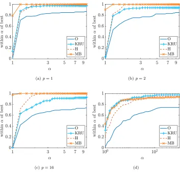
We make use of performance profiles [6] that allow us to easily display, for all ma-trices in the test set, how the scalings affect a performance measure like the condition number. To obtain the performance profile, we first define the performance ratio for scaling k on a given matrix to be the ratio of the performance for scalingk to that of the best performing scaling, out of all of the scaling methods being compared, for that matrix. Throughout, we assume that the performance measure of interest is one for which a smaller number is better. The monotonically increasing functionfscale(α), α∈[1,∞), then measures the proportion of matrices for which the performance ratio for a particular scaling is at most α. Plotting the curvesfscale(α) against αfor the different scalings gives a performance profile that shows which scaling performs best or joint-best (α= 1) and which scalings are near-best (smallα). Additionally, limα→∞ indicates when a scaling fails (say, to produce LandU factors without pivoting) on a matrix for which at least one other scaling does not fail.
4.1. Matrix properties. To assess the row diagonal dominance of a matrix A∈Rn×n, we measure ∆p(A) as in (3.5). The smaller the score, the more diagonally
dominant the matrix. Since all of the matrices in our test set are irreducible, it is not possible for any of them to have a score of zero when the optimal assignment ordering has been applied.
For each matrix in the test set we record ∆p(A) for each of the scaling methods
and forp= 1,2,16. See Figure 4.1(a)–(c). Without scaling many matrices are far from diagonally dominant, but the KRU and H methods are both close to the best method for the vast majority of matrices. Although their performance is nearly identical for p= 1 andp= 2, the H method outperforms the KRU method forp= 16. Theorem 3.8 states that for any matrix A ∈ Rn×n, there exists p0 >0, such that for all p≥ p0, the MB method will be optimal. Thus, for larger values of p, the MB method will outperform all of the other methods. The figure shows that MB outperforms all of the other methods even for the smaller values ofp, although the number of problems for which it is best is larger forp= 16. Note that we also measured column diagonal dominance (the row diagonal dominance measure applied to AT); the results were
similar and so have been omitted.
We additionally note that applying the optimal assignment scaling has a signif-icant impact on diagonal dominance. If the optimal assignment permutation is not applied, there are 19 matrices with zeros on the diagonal. When methods O and KRU are used without first applying the optimal assignment permutation, both suffer from many fails and are the worst-performing methods.
Figure 4.1(d) shows the estimated condition number of the scaled matrices, using the MATLAB functioncondest. All of the scaling methods consistently outperform method O. The KRU and MB methods have similar performance. The H method is also close to these two methods but is slightly weaker at achieving near-best condition numbers, and for some problems it is far from the best scaling.
(a)p= 1 (b)p= 2
[image:21.612.79.432.107.444.2](c)p= 16 (d)
Fig. 4.1. (a)–(c)Performance profile of the row diagonal dominance factor∆p in (3.5) for
p= 1,2,16. (d)Performance profile of the estimated condition numbers.
4.2. Gaussian elimination. In this subsection we examine the effect of the scalings on the performance of Gaussian elimination. We use UMFPACK with the MATLAB interface to compute the LU factors with the symmetric pivoting strategy (to prevent column reordering) and the CHOLMOD fill-reducing ordering option. Otherwise default settings are applied. Three different pivoting options are tested: no pivoting, threshold pivoting with default tolerances, and partial pivoting. We denote by a fail any matrix for which the estimated condition number (using the MATLAB functioncondest) is larger than 1015.
Figure 4.2 shows the condition number of the upper triangular factorU computed during Gaussian elimination. When pivoting is not used, the O method results in very poorly conditioned U factors for several of the problems. The three scaling methods have similar numbers of fails, and the H and MB methods have nearly identical performance; they are typically optimal or near-optimal. With threshold pivoting the pattern is the same except that there are fewer fails, with the H and MB methods computing a reasonably conditioned U factor for all matrices. With partial pivoting the results are much the same as with threshold pivoting, although the MB method
(a) no pivoting (b) threshold pivoting
[image:22.612.80.427.109.446.2](c) partial pivoting
Fig. 4.2.Performance profile of the estimated condition number ofU. Table 4.2
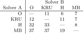
Number of problems for which solver B requires at least50more off-diagonal pivots than solver A for threshold pivoting.
Solver B Solver A O KRU H MB
O — 5 1 2
KRU 17 — 13 1
H 17 13 — 3
MB 25 15 15 —
is optimal for slightly more matrices.
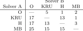
We count the number of off-diagonal pivots (as tabulated by UMFPACK) used in Gaussian elimination. Performance profiles are not appropriate for displaying this data as there are certain problems and scalings for which no off-diagonal pivots are required, so we make use of tables instead. Tables 4.2 and 4.3 show the number of problems for which one solver requires at least 50 fewer off-diagonal pivots than the other solvers. From this we see that when threshold pivoting is applied, method O is the weakest, only winning over another method eight times. KRU and H have similar
[image:22.612.187.326.519.572.2]Table 4.3
Number of problems for which solver B requires at least50more off-diagonal pivots than solver A for partial pivoting.
Solver B Solver A O KRU H MB
O — 11 6 7
KRU 12 — 11 7
H 32 33 — 8
MB 37 37 19 —
performances, with MB being the best performing method. When partial pivoting is used, the ordering of the methods is the same, but the differences between them become more pronounced. Although the H method is closer to the MB method, the MB method wins over the H method 19 times and loses to it only eight times.
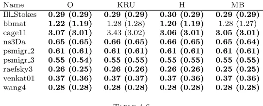
Tables 4.4, 4.5, and 4.6 show the factorization times for the nine matrices for which factorization took longer than 0.25 seconds for all scalings and pivoting strategies. For each matrix we record the average time over 10 runs, and the minimum time out of these 10. We mark with a dash factorizations which ended in breakdown. Table 4.7 also shows the number of row interchanges needed for these factorizations.
Without pivoting the time taken to compute the factorization depends only on the pattern of the matrix. Thus we expect the different scalings to have very similar run-times because the methods will return matrices with the same pattern. The reason for the breakdown of the factorizations of bbmat is not so clear, but this highlights that although the optimal assignment ordering and Hungarian scaling improves the robustness and quality of LU factorizations in many cases, it is not guaranteed to do so.
The effects that determine the time taken to compute a factorization with pivoting are more complex. Performing lots of row interchanges will add to the computation time but may also affect the density of the LU factors. However, in general we find that with threshold pivoting there is still very little difference between the scalings, with the exception of the KRU and MB scalings forbbmat, and the KRU scaling for
cage11. With partial pivoting, method MB wins, being within 5% of the fastest time for seven out of nine problems.
The number of pivots required was generally reduced significantly by applying the optimal assignment permutation. For example, when neither the optimal assignment permutation nor a diagonal scaling is applied to the matrixIll Stokes, threshold piv-oting requires 4948 pivots. However, after applying the optimal assignment ordering, the factorization can be computed without pivoting.
4.3. Iterative solvers. In this subsection we examine the effect of scaling on the performance of iterative solvers with incomplete LU (ILU) preconditioners. For each test matrixA we take the scaled and reordered matrixS=PRDRADCPC and
then compute ILU factorsLU forS using the MATLAB functioniluwith options
setup.type=’ilutp’; setup.droptol=0.01;
which performs threshold ILU with partial pivoting and a drop tolerance of 0.01. Combining the ILU factors with the scaling and permutation matrices results in the preconditioner
M = (D−1R PR−1L)(U PC−1D−1C ).
Next we solve the linear systemAx=busing right-preconditioned GMRES and
Table 4.4
Average factorization time with minimum factorization time in parentheses. Factors are com-puted without pivoting. Numbers in bold represent average times that are within5% of the lowest time for that problem.
Name O KRU H MB
Ill Stokes 0.29 (0.29) 0.29 (0.29) 0.29 (0.29) 0.29 (0.29)
bbmat — — — —
[image:24.612.120.392.143.252.2]cage11 3.02 (3.01) 3.08 (3.07) 3.08 (3.01) 3.09 (3.07) ns3Da 0.65 (0.65) 0.66 (0.65) 0.66 (0.65) 0.65 (0.64) psmigr 2 0.61 (0.61) 0.61 (0.61) 0.61 (0.61) 0.61 (0.61) psmigr 3 0.55 (0.55) 0.55 (0.55) 0.55 (0.55) 0.56 (0.55) raefsky3 0.26 (0.26) 0.26 (0.26) 0.26 (0.26) 0.26 (0.25) venkat01 0.37 (0.36) 0.37 (0.37) 0.37 (0.37) 0.37 (0.36) wang4 0.28 (0.28) 0.28 (0.28) 0.28 (0.28) 0.28 (0.28)
Table 4.5
Average factorization time with minimum factorization time in parentheses. Factors are com-puted with threshold pivoting. Numbers in bold represent average times that are within5% of the lowest time for that problem.
Name O KRU H MB
[image:24.612.121.392.297.407.2]Ill Stokes 0.29 (0.29) 0.29 (0.29) 0.30 (0.29) 0.29 (0.29) bbmat 1.22 (1.19) 1.28 (1.28) 1.20 (1.19) 1.28 (1.27) cage11 3.07 (3.01) 3.43 (3.02) 3.06 (3.01) 3.05 (3.01) ns3Da 0.65 (0.65) 0.66 (0.65) 0.66 (0.65) 0.65 (0.64) psmigr 2 0.61 (0.61) 0.61 (0.61) 0.61 (0.61) 0.61 (0.61) psmigr 3 0.55 (0.54) 0.55 (0.55) 0.55 (0.55) 0.55 (0.55) raefsky3 0.26 (0.25) 0.26 (0.26) 0.26 (0.26) 0.25 (0.25) venkat01 0.37 (0.36) 0.37 (0.37) 0.37 (0.36) 0.37 (0.36) wang4 0.28 (0.28) 0.28 (0.28) 0.28 (0.28) 0.28 (0.28)
Table 4.6
Average factorization time with minimum factorization time in parentheses. Factors are com-puted with partial pivoting. Numbers in bold represent average times that are within5% of the lowest time for that problem.
Name O KRU H MB
[image:24.612.110.400.450.559.2]Ill Stokes 7.09 (7.07) 5.31 (5.30) 5.57 (5.55) 2.43 (2.41) bbmat 11.69 (11.61) 5.99 (5.92) 10.07 (10.04) 3.91 (3.89) cage11 3.09 (3.08) 3.03 (3.01) 3.01 (3.00) 3.01 (3.01) ns3Da 1.44 (1.42) 1.25 (1.25) 2.10 (2.10) 1.82 (1.82) psmigr 2 1.67 (1.67) 1.70 (1.69) 1.96 (1.96) 1.15 (1.15) psmigr 3 0.55 (0.54) 0.55 (0.55) 0.55 (0.55) 0.56 (0.55) raefsky3 1.30 (1.30) 0.33 (0.33) 0.53 (0.53) 0.65 (0.65) venkat01 0.38 (0.37) 0.37 (0.37) 0.37 (0.37) 0.37 (0.36) wang4 0.28 (0.28) 0.30 (0.30) 0.28 (0.28) 0.28 (0.28)
Table 4.7
The number of row interchanges used by UMFPACK when threshold and partial pivoting are used.
Name Threshold Partial
O KRU H MB O KRU H MB
Ill Stokes 0 0 0 0 7215 4162 3789 3003 bbmat 149 112 132 128 8881 5314 6729 2988
cage11 0 0 0 0 0 0 0 0
ns3Da 2 2 2 2 1661 1468 1352 1165
psmigr 2 16 13 5 6 913 903 905 714
psmigr 3 0 0 0 0 2 2 0 0
raefsky3 0 0 0 0 1551 608 601 1166
venkat01 0 0 0 0 16425 179 13135 186
wang4 0 0 0 0 0 7 0 2
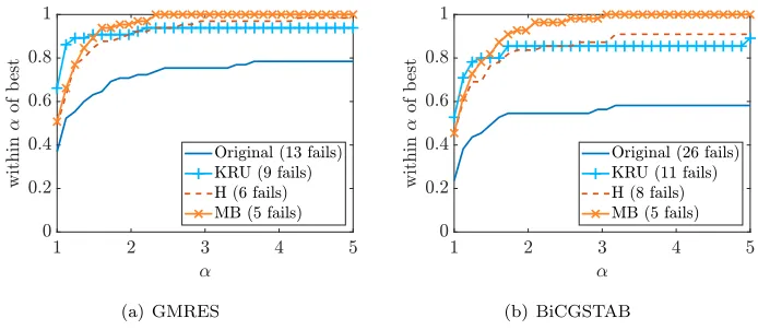
(a) GMRES (b) BiCGSTAB Fig. 4.3.Performance profiles of number of iterations needed for convergence.
preconditioned BiCGSTAB, wherebis chosen so that the exact solution is a vector of ones. We use the MATLAB functionsgmres(without restarts) andbicgstab, with a tolerance of 10−6, and a maximum of min{n,1000} iterations. If either method fails to converge below the tolerance within the maximum number of iterations, then we record a fail. Many of the problems in the test set are solved very easily, so we omit any matrix for which the O method converges in fewer than 10 iterations. This leaves 65 problems for GMRES and 55 problems for BiCGStab.
Figure 4.3 shows the number of iterations needed for the different scaling strate-gies. All of the scaling methods significantly outperform method O when GMRES is used. Method MB outperforms method H by a small margin. Method KRU is slightly better than method MB at producing very low numbers of iterations but is less re-liable, resulting in four more fails. The pattern is the same for BiCGSTAB except that the advantage of the KRU method for low numbers of iterations is smaller and the advantage of the MB method for reliability is greater, with four fewer fails than KRU.
5. Conclusion. We have introduced max-balanced Hungarian scaling, which is applied to a matrix A ∈ Cn×n in two stages. First we apply a Hungarian scaling and optimal assignment reorderingH =P D1AD2, such that |hij| ≤1 and|hii|= 1
for i = 1, . . . , n. The permutation matrixP and diagonal matrices D1, D2 can be obtained using standard algorithms such as the HSL code MC64 [14]. The second stage is to apply a max-balancing similarity scalingM =S−1HS, such that for all I ⊂ {1, . . . , n} we have
(5.1) max
i∈I,j6∈I|mij|= maxi∈I,j6∈I|mji|.
The diagonal matrixS can be obtained using Algorithm 3.10, which was first intro-duced by Schneider and Schneider [20], with a more efficient implementation given by Young, Tarjan, and Orlin [22].
In Theorem 3.6 we proved that max-balancing preserves the properties of a Hun-garian scaling, so that M satisfies |mij| ≤1 and |mii| = 1 for i = 1, . . . , n as well
as (5.1). In Theorem 3.8 we proved thatM is the most diagonally dominant matrix out of all possible scalings and reorderings ofA, when viewed through thep-norm for sufficiently largep, up to multiplication by permutation matrices that switch between