PROCESSES ON GRAPHS. II. TWO-DIMENSIONAL LATTICE
ERNESTO ESTRADA, EHSAN HAMEED, MATTHIAS LANGER, AND ALEKSANDRA PUCHALSKA
Abstract. In this paper we consider a generalized diffusion equation on a square lattice corresponding to Mellin transforms of thek-path Laplacian. In particular, we prove that superdiffusion occurs when the parametersin the Mellin transform is in the interval (2,4) and that normal diffusion prevails whens >4.
1. Introduction
Many physical systems are best represented by graphs G= (V, E), where the set of nodes (vertices) V represents the entities of the system and the set of edges
E describes the interactions between these entities [13]. Among those systems we can mention atomic and molecular ones as well as complex networks, which include a vast range of complex systems embracing biological, social, ecological, infrastructural and technological ones. Diffusion-like processes, such as diffusion, reaction-diffusion, synchronization, epidemic spreading, etc., are ubiquitous in those previously mentioned systems [6]. Apart from the normal diffusive processes, where the mean square displacement (MSD) of the diffusive particle scales linearly with time, there are many real-world examples where anomalous diffusion takes place. In these anomalous diffusive processes, MSD scales nonlinearly with time giving rise to subdiffusive and superdiffusive processes [29].
In Part I [15] of this series we introduced a new theoretical framework to study superdiffusive processes on graphs. In that work we considered transformations of the so-called k-path Laplace operators Lk. The latter are defined in a similar way as the standard graph Laplacian, but they take only nodes into account whose distance is equal to k; here the distance is measured as the length of the shortest path connecting two nodes. Hence Lk describes hops to nodes at distance k. The above mentioned transformations of Lk are combinations of the formP
∞
k=1ckLk with some non-negative coefficients ck. This combination describes interactions with all nodes where different strengths are used for nodes at different distances. In general, one uses a sequence ck that is decreasing in k. In particular, in [15] we considered the Mellin transform ofLk, which is obtained by choosingck =k−s with some positive parameters. The choice of the transformation has proved to be crucial in determining the diffusive behaviour. In [15] we studied, in particular, the one-dimensional path graph. We proved that superdiffusion appears when a Mellin transform of thek-path Laplace operators is considered withssatisfying 1< s <3, while for s >3 normal diffusion is obtained; the latter occurs also if one considers different transformations ofLk like the Laplace and factorial transforms.
This new method adds new values to the already existing ones for modelling anomalous diffusion. Among such existing methods we should mention the use of random walks with L´evy flights (RWLF) [12, 34, 38, 30] and the use of the fractional
2010Mathematics Subject Classification. 47B39; 60J60, 05C81.
Key words and phrases. k-path Laplacian, anomalous diffusion, square lattice.
diffusion equation (FDE) [27, 36, 23, 16]. While the first method is easy to use for computer simulations, the second is preferred for analytical studies. However, there are different types of definitions of fractional derivatives, such as the Caputo frac-tional operator and the Riemann–Liouville fracfrac-tional operator [32], which then have different interpretations and adapt differently to the different physical phenomena studied with them (see [20, 26]). The k-path Laplace operators allow the deriv-ation of analytical results as the FDE but use a unique framework which is very similar to the one traditionally used in graph and network theory. It also allows an easy computational implementation in the form of a random multi-hopper on graphs [14].
The goal of the current work is to study the solutions of the generalized diffu-sion equation in 2D graphs. In particular, we focus our attention on the abstract Cauchy problem in an infinite square lattice. Square lattices are ubiquitous in many real-world physical systems. It is frequently used to describe the spin-1/2 antifer-romagnetic Heisenberg model in a variety of materials [28, 19, 3, 11]. It is also the preferred model for two-dimensional (2D) gases and optical lattices [5, 21, 18, 1, 25]. Recently, square lattices of superconducting qubits have been used for error cor-recting codes in quantum computers [9]. A very interesting discovery has been the experimental finding that the native architecture of certain photosynthetic mem-branes have square lattice shapes [35, 4, 10]. This finding is very relevant for the current work as the existence of long-range interactions (LRI) is well documented for light-harvesting complexes [17, 7, 8]. The existence of LRI like the ones math-ematically described by thek-path Laplace operators considered here are well doc-umented for other systems previously mentioned here, such as cold atomic clouds, helium Rydberg atoms and cold Rydberg gases [2, 22, 37]. Note also that anom-alous diffusion has been observed for ultracold atoms in 2D and 3D lattices [33]. Consequently, the study of a generalized diffusion model on square lattices and proving the conditions for which superdiffusive behaviour exists on them is of great theoretical importance due to the many physical processes involved.
The main result of the current paper is contained in Theorem 4.7, which describes the asymptotic behaviour of the generalized diffusion equation corresponding to the Mellin-transformed k-path Laplacian. We prove that superdiffusion occurs when 2 < s < 4 and that normal diffusion prevails when s > 4. More precisely, we consider the time evolution of the solution of the generalized diffusion equation with initial condition concentrated at one point. As time t tends to infinity, the spread of the solution (e.g. measured by the full width at half maximum) grows like tκ with κ= 12 when s > 4, which is normal diffusion, and with κ > 12 when 2< s <4, which is a superdiffusive behaviour.
Let us give a brief outline of the contents of the paper: in Section 2 we recall results from Part I [15]. In Section 3 we study the solution of the generalized diffusion equation and give an integral representation (Theorem 3.3). Finally, in Section 4 we investigate the asymptotic behaviour of the solution as time tends to infinity. In particular, we formulate and prove or main result (Theorem 4.7). Finally, we examine the behaviour of finite truncations, PN
k=1k
−sL
k of the Mellin transforms. Although normal diffusion occurs in this case, the diffusion speed can be made arbitrarily large if s∈(2,4) andN is large enough; see Remark 4.9.
2. Preliminaries
At the beginning let us briefly recall some of the results given in the first part [15] of this article. Let Γ = (V, E) be an undirected, locally finite graph with set of verticesV and set of edgesE. Moreover, letdbe the distance metric onV, i.e. let
degree of a vertex v∈V:
δk(v) = #{w∈V :d(v, w) =k}. (2.1) Let `2(V) be the Hilbert space of square-summable functions on V with inner product
hf, gi=X v∈V
f(v)g(v), f, g∈`2(V).
For k ∈ N we consider the k-path Laplacian, which is an operator in `2(V) and defined by
Lkf
(v) := X w∈V:d(v,w)=k
f(v)−f(w)
, f ∈dom(Lk), (2.2)
with maximal domain dom(Lk), i.e.
dom(Lk) =
(
f ∈`2(V) :X v∈V
X
w∈V:d(v,w)=k
f(v)−f(w)
2
<∞
) .
The following properties were proved in the first part of the paper.
Theorem 2.1. [15, Theorem 2.2] For each k ∈ N the k-path Laplacian Lk is a
self-adjoined operator in `2(V). Furthermore, the operator L
k is bounded if and
only if the function δk:V →Nis bounded.
Now let us consider an Abstract Cauchy Problem of the form
u0(t) =−Lu(t), u(0) = ˚u, (2.3) whereLis some operator in`2(V). Similarly to the classical description of Brownian motion, the solution to the system (2.3) with L = Lk, when rescaled properly, converges to the normal distribution as time tends to infinity. In order to build the model in which interaction among all vertices in a graph that are joined by a path are taken into account, we use the differential equation (2.3) with an operator L
given by a transformedk-path Laplacian operator:
L=
∞ X
k=1
ckLk (2.4)
with some coefficients ck ∈C.
The main goal is to examine the existence of superdiffusion in the process de-scribed by (2.3) with an operator Las in (2.4). In [15] we considered three trans-forms: the Laplace, the factorial and the Mellin transforms, which differ in the rate of convergence to zero of their coefficients. It appeared that for the first two the probabilities of big jumps are too small for superdiffusion to arise and a significant result happens only for the Mellin transform. In the current paper we therefore con-centrate on the Mellin transform. Let us recall the definition and some properties of the latter in the following theorem from [15].
Theorem 2.2. [15, Theorem 3.1]Let us consider an infinite graphΓwhich is locally finite and such that its k-path degreeδk, defined in (2.1), satisfies the condition
δk,max:= max{δk(v) :v∈V} ≤Ckα (2.5)
for some α≥0 andC >0. Then the Mellin-transformedk-path Laplacian
LM,s:=
∞ X
k=1 1
ksLk (2.6)
is a well-defined, bounded operator in `2(V) fors∈C with Res > α+ 1, and the
One can easily find examples of graphs for which (2.5) is satisfied and hence the operator LM,s is bounded, e.g. a path graph or a square lattice where δk,max equals 2 and 4k, respectively. On the other hand, condition (2.5) is violated for the Cayley trees with degree of the non-pendant node equal tor∈N,r≥3, for which δk,max=r(r−1)k−1.
3. Existence and time evolution of the Mellin transform of the k-path Laplacian on the square lattice
Let us consider the square lattice, i.e. the graph Γ =P∞×P∞= (V, E) with vertices V =Z2 and edges connecting vertices (i, j) and (m, n) when|i−m|+|j−n|= 1.
We usually write (ux,y)x,y∈Z for functions onV.
OnP∞×P∞ thek-path LaplacianLk, defined in (2.2), is given by
(Lku)x,y = 4kux,y− k−1
X
j=0
h
ux+k−j,y+j+ux−k+j,y−j+ux−j,y+k−j+ux+j,y−k+j
i ,
x, y∈Z, u∈`2(V).
Clearly, Lk is a bounded operator. Form, n∈Zletσm,n :`2(V)→`2(V) be the shift operator defined by
(σm,nu)x,y =ux+m,y+n, x, y ∈Z.
ThenLk can be written as
Lk = 4kI− k−1
X
j=0
σk−j,j+σ−k+j,−j+σ−j,k−j+σj,−k+j. (3.1)
Let us consider the following Fourier transform, which is a unitary operator and which is defined by
F :`2(V)→L2 [−π, π]2 ,
(Fu)(p, q) = 1 2π
X
x,y∈Z
ux,yeipxeiqy, p, q∈[−π, π], u∈`2(V),
and whose inverse given by
(F−1f) x,y =
1 2π
ˆ π
−π
ˆ π
−π
f(p, q)e−ipxe−iqydpdq, x, y ∈Z, f ∈L2 [−π, π]2 .
Since
(Fσm,nu)(p, q) = 1 2π
X
x,y∈Z
ux+m,y+neipxeiqy= 1 2π
X
x,y∈Z
ux,yeip(x−m)eiq(y−n)
=e−ipme−iqn(Fu)(p, q),
we have
Fσm,nF−1f
(p, q) =e−i(pm+qn)f(p, q), p, q∈[−π, π], f ∈L2 [−π, π]2 . (3.2) Together with (3.1) we obtain that Lk is unitarily equivalent to a multiplication operator; more precisely, the following lemma is true.
Lemma 3.1. With the notations from above we have
FLkF−1f
(p, q) =lk(p, q)f(p, q), p, q∈[−π, π], f ∈L2 [−π, π]2
where
lk(p, q) =
4k−isinp· e
ikp−e−ikp
−sinq· eikq−e−ikq
cosp−cosq , |p| 6=|q|,
4k+icotp· eikp−e−ikp
−k eikp+e−ikp
, |p|=|q| 6= 0, π,
0, p=q= 0,
4k 1−(−1)k
, |p|=|q|=π.
Moreover, lk is continuous and even in bothpandq, and the following inequalities
hold:
0≤lk(p, q)≤8k, p, q∈[−π, π], (3.4)
l1(p, q)>0, (p, q)∈[−π, π]2\ {(0,0)}. (3.5)
Proof. It follows from (3.1) and (3.2) that (3.3) holds with
lk(p, q) = 4k− k−1
X
j=0
h
e−i[(k−j)p+jq]−e−i[(−k+j)p−jq]
−e−i[−jp+(k−j)q]−e−i[jp+(−k+j)q]i
= 4k−e−ikp
k−1
X
j=0
eij(p−q)+eikp
k−1
X
j=0
e−ij(p−q)
+e−ikq
k−1
X
j=0
eij(p+q)+eikq
k−1
X
j=0
e−ij(p+q). (3.6)
When|p| 6=|q|we can rewrite this as follows:
lk(p, q) = 4k−
e−ikp−e−ikq 1−ei(p−q) −
eikp−eikq 1−e−i(p−q)−
e−ikq−eikp 1−ei(p+q) −
eikq−e−ikp 1−e−i(p+q)
= 4k−eikp
1
1−e−ip+iq − 1 1−eip+iq
−e−ikp
1
1−eip−iq − 1 1−e−ip−iq
+eikq
1
1−e−ip+iq − 1 1−e−ip−iq
+e−ikq
1
1−eip−iq − 1 1−eip+iq
.
The expressions within the brackets can be simplified, e.g. 1
1−e−ip+iq − 1 1−eip+iq =
e−ip+iq−eip+iq 1−e−ip+iq−eip+iq+e2iq
= e
−ip−eip
e−iq−e−ip−eip+eiq =
isinp
cosp−cosq.
Hence
lk(p, q) = 4k−eikp
isinp
cosp−cosq+e
−ikp isinp cosp−cosq
+eikq isinq
cosp−cosq−e
−ikq isinq cosp−cosq
= 4k− i
cosp−cosq h
For the case when |p|=|q|note thatlk is continuous by (3.6). Writelk as
lk(p, q) = 4k−i
f(p)−f(q)
g(p)−g(q)
with f(p) = sinp·(eikp−e−ikp) and g(p) = cosp. The Generalized Mean Value Theorem implies that
lk(p, q) = 4k−i
f0(ξ)
g0(ξ)
with ξbetweenpandq. Hence
lk(p, p) = lim
q→plk(p, q) = 4k−i
f0(p)
g0(p)
= 4k−icosp·(e
ikp−e−ikp) +iksinp·(eikp+e−ikp) −sinp
= 4k+icotp· eikp−e−ikp
−k eikp+e−ikp
. (3.7)
The relation lk(0,0) = 0 follows from (3.6), and the value for lk(p, q) when|p| = |q|=πfollows from (3.7) by taking the limitp→π.
That lk is even inpandqis clear. SinceLk is a non-negative operator in`2(V) by [15, Section 2], the functionlk is non-negative. The upper bound forlk in (3.4) follows from (3.6).
Finally, to show (3.5) rewritel1; for|p| 6=|q|we have
l1(p, q) = 4 + 2
sin2p−sin2q
cosp−cosq = 4−2(cosp+ cosq), (3.8)
which extends to all p, q ∈ [−π, π] by continuity. The right-hand side of (3.8) is
strictly positive unlessp=q= 0.
Let us now consider the Mellin transformation of thek-path LaplaciansLk, i.e. the operator
LM,s=
∞ X
k=1 1
ksLk;
see (2.6). Since kLkk ≤ 8k by Lemma 3.1, the series converges in the operator norm when s > 2. As the next lemma shows, the operator LM,s is also unitarily equivalent to a multiplication operator in L2([−π, π]2). In order to formulate this lemma, we have to recall the definition of the polylogarithm. Fors∈Cthe function Lisis defined by
Lis(z) :=
∞ X
k=1
zk
ks, |z|<1,
and by analytic continuation to C\[1,∞) with 1 being a branch point; see, e.g. [31, 25.12.10].
Lemma 3.2. Fors >2 we have
FLM,sF−1f
where
lM,s(p, q) :=
∞ X
k=1 1
kslk(p, q) (3.10)
=
4ζ(s−1) + gs(p)−gs(q)
cosp−cosq , |p| 6=|q|,
4ζ(s−1)−2 cotp·Im Lis(eip)−2 Re Lis−1(eip), |p|=|q| 6= 0, π,
0, p=q= 0,
4 1−(−1)k
ζ(s−1), |p|=|q|=π,
with
gs(p) := 2 sinp·Im Lis(eip). (3.11)
The function lM,s is continuous and even in both p and q, and the following
in-equalities hold:
0≤lM,s(p, q)≤8ζ(s−1), p, q∈[−π, π], (3.12)
lM,s(p, q)>0, (p, q)∈[−π, π]2\ {(0,0)}. (3.13)
Proof. It follows from Lemma 3.1 that (3.9) holds with lM,s defined as in (3.10). When|p| 6=|q|, we have
lM,s(p, q) =
∞ X k=1 1 ks
4k−isinp· e
ikp−e−ikp
−sinq· eikq−e−ikq
cosp−cosq
= 4 ∞ X k=1 1
ks−1 −
i
cosp−cosq
sinp·
∞ X k=1 1 ks
(eip)k−(e−ip)k
−sinq·
∞ X k=1 1 ks
(eiq)k−(e−iq)k
= 4ζ(s−1)− i cosp−cosq
h
sinp·Lis(eip)−Lis(e−ip)
−sinq·Lis(eiq)−Lis(e−iq)i,
which proves the formula forlM,sin the first case. Now assume that|p|=|q| 6= 0, π. Then
lM,s(p, q) =
∞ X k=1 1 ks
4k+icotp· eikp−e−ikp−k eikp+e−ikp = 4 ∞ X k=1 1
ks−1+icotp·
∞ X k=1 1 ks
(eip)k−(e−ip)k−
∞ X
k=1 1
ks−1
(eip)k+ (e−ip)k
= 4ζ(s−1) +icotp· Lis(eip)−Lis(e−ip)
−Lis−1(eip)−Lis−1(e−ip). The remaining cases are clear.
SinceLM,s is a bounded operator, the Cauchy problem
u0(t) =−LM,su(t), t >0, (3.14)
u(0) = ˚u (3.15)
has a unique solution, which is given by
u(t) =e−tLM,s˚u, t≥0.
It follows from Lemma 3.2 that
Fe−tLM,sF−1f(p, q) =e−tlM,s(p,q)f(p, q),
t≥0, p, q∈[−π, π], f ∈L2 [−π, π]2.
(3.16)
Using this relation and the fact that lM,s is even one can easily show the following theorem; cf. [15, Theorem 5.2] for the case of the infinite path graph. For the formulation of the theorem let em,n∈`2(V) be the vector defined by
(em,n)x,y=
(
1, m=x, n=y,
0, otherwise. (3.17)
Theorem 3.3. Let s >2 and˚u∈`2(V). The unique solution of (3.14),(3.15) is
given by
ux,y(t) = 1 4π2
X
m,n∈Z
˚um,n
ˆ π
−π
ˆ π
−π
ei[(x−m)p+(y−n)q]e−tlM,s(p,q)dpdq, x, y∈ Z.
In particular, for˚u=e0,0 we obtain
ux,y(t) = 1 4π2
ˆ π
−π
ˆ π
−π
ei(xp+yq)e−tlM,s(p,q)dpdq, x, y∈
Z. (3.18)
4. Diffusion and superdiffusion for Mellin-transformed k-path Laplacian on a square lattice
In this section we examine the long-time behaviour of the solution to the Cauchy problem generated by the Mellin-transformedk-path Laplacian. The main result is contained in Theorem 4.7. To prove this theorem we first examine the asymptotic behaviour of the functionlM,s(see Figure 4.1) as the arguments tend to zero, which is contained in Proposition 4.5. The discussion is based on similar considerations undertaken for the path graph in [15], but the arguments are more subtle. We start with a simple lemma, which is used a couple of times below.
Lemma 4.1. Letb >0, letf : (0, b)→Rbe differentiable and assume that
|f0(t)| ≤Ctα, t∈(0, b),
for some C >0 andα≥1. Then
f(p)−f(q)
p2−q2
≤ C 2 max
pα−1, qα−1 , p, q∈(0, b), p6=q.
Proof. Define the function g(x) := f(√x), x∈(0, b2). Let p, q ∈ (0, b) such that
p6=qand setx:=p2,y:=q2. Then
f(p)−f(q)
p2−q2
=
g(x)−g(y)
x−y
=|g0(ξ)| (4.1)
for some ξbetweenxand y by the Mean Value Theorem. Since√ξ≤max{p, q}, we obtain that
|g0(ξ)|=
f0(√ξ) 2√ξ
≤ C( √
ξ)α 2√ξ ≤
C
2 max
pα−1, qα−1 ,
(a) s= 2.1 (b)s= 5
[image:9.595.133.451.120.504.2](c) lM,s restricted top=qfors= 2.1 (blue) ands= 5 (red), respectively
Figure 4.1. The graph of the functionlM,son the square [−π, π]2 for the parameters s = 2.1 (a) and s = 5 (b), respectively. The third graph (c) shows the behaviour of both solutions s= 2.1 and
s= 5 restricted to the linep=q.
In the next three lemmas we prove auxiliary asymptotic results, which are used to obtain the asymptotic behaviour oflM,s in Proposition 4.5.
Lemma 4.2. We have
1
cosp−cosq =−
2
p2−q2
1 + 1 12 p
2+q2
+R1(p, q)
, p, q∈[−π, π], |p| 6=|q|.
where
R1(p, q) = O p4+q4
, p, q→0, |p| 6=|q|.
Proof. We write
cosp= 1−p 2
2 +
where f0(p) = O(p5),p→0. Forp, q∈(0, π] withp6=qwe have
cosp−cosq=−p 2−q2
2 +
p4−q4
24 +f(p)−f(q)
=−1 2(p
2−q2)
1− 1 12 p
2+q2
−2f(p)−f(q)
p2−q2
=−1 2(p
2−q2)
1− 1 12 p
2+q2
+ O p4+q4
, p, q→0,
where the last relation follows from Lemma 4.1. Now the claim is obtained by taking inverses on both sides and extending the result to non-positive p, q by continuity
and symmetry.
Lemma 4.3. Lets∈(2,∞)\ {4}. Then
2 Im Lis(eip)=−Cs 2 p
s−1+ 2ζ(s−1)p−ζ(s−3)
3 p
3+R2,s(p), p∈(0,2π),
where
Cs:=
− 2π
Γ(s) sin(sπ2), s /∈2Z,
0, s∈2Z,
(4.2)
and
R2,s(p) = O(p5) and R02,s(p) = O(p
4), p&0, if s6= 6,
and
R2,s(p) = O p5|lnp|
and R02,s(p) = O p4|lnp|
, p&0, if s= 6.
Proof. First lets∈(2,∞)\N. It follows from [31, 25.12.12] that, forp∈(0,2π),
2 Im Lis(eip)
= 2 Im
"
Γ(1−s)(−ip)s−1+
∞ X
n=0
ζ(s−n)(ip) n
n!
#
= 2 Im
"
Γ(1−s)ps−1e−(s−1)π2i+
∞ X
n=0
ζ(s−n)i npn
n!
#
=−2Γ(1−s) sin(s−1)π 2
ps−1+ 2
∞ X
l=0
ζ(s−2l−1) (−1) l
(2l+ 1)!p 2l+1
=−Cs 2 p
s−1+ 2ζ(s−1)p−ζ(s−3)
3 p
3+R2,s(p),
where
Cs= 4Γ(1−s) sin
(s−1)π 2
=4πsin (s−1) π 2
Γ(s) sin(sπ) =−
4πcos(sπ2) Γ(s) sin(sπ)
=− 2π
Γ(s) sin(sπ2) and
R2,s(p) = 2
∞ X
l=2
ζ(s−2l−1) (−1) l
(2l+ 1)!p 2l+1.
This relation extends tosbeing an odd integer withs≥3. Moreover,R2,ssatisfies
R2,s(p) = O(p5) and R02,s(p) = O(p
Now lets∈ {6,8, . . .} and set
Hn= n
X
j=1 1
j.
From [24, p. 131] we obtain, again forp∈(0,2π),
2 Im Lis(eip)
= 2 Im
"
(ip)s−1 (s−1)!
Hs−1−Log(−ip)
+
∞ X
n=0 n6=s−1
ζ(s−n)(ip) n
n!
#
= 2 Im
"
(−1)s2−1ips−1 (s−1)!
Hs−1−lnp+i
π 2 + ∞ X n=0 n6=s−1
ζ(s−n)i npn
n!
#
= 2(−1)
s
2−1 (s−1)! p
s−1 H
s−1−lnp
+ 2
∞ X
l=0 l6=s
2−1
ζ(s−2l−1) (−1) l
(2l+ 1)!p 2l+1
= 2ζ(s−1)p−ζ(s−3)
3 p
3+R2,s(p),
where
R2,s(p) =
2(−1)s2−1 (s−1)! p
s−1 H
s−1−lnp
+ 2 X
l=2 l6=s
2−1
ζ(s−2l−1) (−1) l
(2l+ 1)!p 2l+1,
which satisfies
R2,s(p) = O(p5) and R02,s(p) = O(p4), p&0, if s≥8,
and
R2,s(p) = O p5|lnp|
and R02,s(p) = O p4|lnp|
, p&0, if s= 6.
This finishes the proof in the case when s∈ {6,8, . . .}. Lemma 4.4. Let s∈(2,∞)\ {4} and let gs be defined as in (3.11) andCs as in (4.2). Then
gs(p) =−Cs 2 p
s+ 2ζ(s−1)p2−ζ(s−1) +ζ(s−3)
3 p
4+R3,s(p),
where R3,s satisfies
R03,s(p) =
O(ps+1), s∈(2,4),
O(p5), s∈(4,∞)\ {6}, O p5|lnp|
, s= 6,
(4.3)
as p&0.
Proof. Write sinp=p−p63 +Rsin(p). From Lemma 4.3 we obtain that
gs(p) = 2 sinp·Im Lis(eip)
=
p−p
3
6 +Rsin(p)
−Cs 2 p
s−1
+ 2ζ(s−1)p−ζ(s−3)
3 p
3
+R2,s(p)
=−Cs 2 p
s+ 2ζ(s
−1)p2−ζ(s−1) +ζ(s−3)
3 p
where
R3,s(p) = Cs 12p
s+2−Cs 2 p
s−1Rsin(p) + 2ζ(s−1)pRsin(p)
+ζ(s−3) 18 p
6−ζ(s−3)
3 p
3Rsin(p) + sinp·R2,s(p), which satisfies
R03,s(p) = O(ps+1) + O(p5) + O R2,s(p)
+ O pR2,s0 (p) .
The latter relation yields (4.3).
In the next proposition we consider the asymptotic behaviour of the function
lM,s around the origin. In particular, we observe that the behaviour differs for the two casess∈(2,4) ands∈(4,∞). For the case whens= 4 the behaviour is more complicated and involves a logarithmic term; we do not consider this case in the following.
Proposition 4.5. Let s∈(2,∞)\ {4}, letlM,s be as in (3.10)andCsas in (4.2).
Moreover, define
h1,s(p, q) :=
Cs
|p|s− |q|s
p2−q2 , |p| 6=|q|,
sCs 2 |p|
s−2, |p|=|q|,
h2,s(p, q) :=ζ(s−1) + 2ζ(s−3)
3 (p
2+q2).
Then
lM,s(p, q) =h1,s(p, q) +h2,s(p, q) +Rs(p, q), p, q∈[−π, π],
where
Rs(p, q) = O pα+qα
, p, q→0,
with
α=
(
min{s,4}, s6= 6,
4−ε, s= 6,
with an arbitrary ε >0. In particular, we have
lM,s(p, q) =
h1,s(p, q) + O(ps+qs), s∈(2,4), h2,s(p, q) + O(p4+q4), s∈(4,∞)\ {6},
h2,s(p, q) + O(p4−ε+q4−ε), s= 6,
as p, q→0 with arbitraryε >0 whens= 6.
Proof. Letp, q∈(0, π] such thatp6=q. From Lemmas 3.2, 4.2 and 4.4 we obtain
lM,s(p, q) = 4ζ(s−1) + gs(p)−gs(q) cosp−cosq
= 4ζ(s−1)− 2
p2−q2
1 + 1 12 p
2+q2
+R1(p, q)
×
×
−Cs 2 (p
s−qs) + 2ζ(s−1)(p2−q2)−ζ(s−1) +ζ(s−3)
3 p
4−q4
+R3,s(p)−R3,s(q)
= 4ζ(s−1) +
1 + 1 12 p
2+q2
+R1(p, q)
·
Cs
ps−qs
p2−q2
−4ζ(s−1) +2 3
ζ(s−1) +ζ(s−3)(p2+q2)−2R3,s(p)−R3,s(q)
p2−q2
=Cs
ps−qs
p2−q2+
2
3
ζ(s−1) +ζ(s−3)−1
3ζ(s−1)
(p2+q2) +Rs(p, q),
where
Rs(p, q) =Cs
1
12 p 2+q2
+R1(p, q)
ps−qs
p2−q2
+R1(p, q)
−4ζ(s−1) + 2 3
ζ(s−1) +ζ(s−3)(p2+q2)
+ 1 18
ζ(s−1) +ζ(s−3)(p2+q2)2
−2
1 + 1 12 p
2+q2
+R1(p, q)
R
3,s(p)−R3,s(q)
p2−q2 . It follows from Lemma 4.4 that
R03,s(p) = O(pβ) where β=
(
min{s+ 1,5}, s6= 6,
5−ε, s= 6,
(4.4)
for arbitraryε >0. Lemma 4.1 implies that
ps−qs
p2−q2 = O p
s−2+qs−2
, q, p→0, p6=q,
and
R3,s(p)−R3,s(q)
p2−q2 = O(p
β−1), q, p
→0, p6=q,
where β is as in (4.4). The error termRssatisfies
Rs(p, q) = O pα+qα, p, q→0, p6=q,
where
α=
(
min{s,4}, s6= 6,
4−ε, s= 6,
with an arbitraryε >0. SincelM,s,h1,sandh2,sare continuous and even inpand
q, the result extends to allp, q∈[−π, π].
The next lemma is the key lemma about the long-time behaviour of the solu-tion of the Cauchy problem; it is a generalizasolu-tion of [15, Lemma 6.1] to the two-dimensional setting. It is more subtle than the one-two-dimensional case, but a further generalization tondimensions is straightforward.
Lemma 4.6. Let α > 0 and let l : [−π, π]2 →
R be a continuous function that
satisfies
l(p, q)>0, (p, q)∈[−π, π]2\ {(0,0)} (4.5)
and can be written as
l(p, q) =h(p, q) +R(p, q)
where the continuous function h:R2→
Rsatisfies
h(rp, rq) =rαh(p, q), r >0, p, q∈R,
and
R(p, q) = o |p|α+|q|α
Define the function
f(x, y, t) := 1 4π2
π
ˆ
−π π
ˆ
−π
ei(xp+yq)e−tl(p,q)dpdq, x, y∈R.
Then
tα2f t
1
αξ, t
1
αη, t→ 1
4π2
∞ ˆ
−∞ ∞ ˆ
−∞
ei(ξv+ηw)e−h(v,w)dvdw=:F(ξ, η), (4.7)
t→ ∞, uniformly in ξ, η∈R.
Hence
f(x, y) =t−2αF t−
1
αx, t−
1
αy+ o t−
2
α, (4.8)
t→ ∞, uniformly in x, y∈R.
Proof. Let us first show that there existsC >0 such that
l(p, q)≥C |p|α+|q|α
, p, q∈[−π, π]. (4.9)
For fixed (p, q)∈R2\ {(0,0)}we have
l(rp, rq) =rαh(p, q) + o(rα), r&0,
which, together with (4.5) implies thath(p, q)>0 for (p, q)∈R2\ {(0,0)}. Set
C1:= min
|p|α+|q|α=1h(p, q),
which is a positive number. Let (p, q)∈R2\ {(0,0)} and set r:= (|p|α+|q|α)
1
α.
Then
h(p, q) =hrp r, r
q r
=rαhp r,
q r
≥C1rα
and hence
h(p, q)≥C1 |p|α+|q|α
, p, q∈R. (4.10)
Together with (4.6), this implies that
l(p, q)≥C1 2 |p|
α+|q|α
, p, q∈R such that |p|α+|q|α≤r0
for some r0>0. Sincel is continuous and satisfies (4.5), we obtain (4.9).
Forξ, η∈Randt >0 we can use the substitutionv=tα1p,w=tα1qto obtain
tα2f t
1
αξ, t
1
αη, t=t
2
α 1
4π2 π
ˆ
−π π
ˆ
−π
eit
1
α(ξp+ηq)e−tl(p,q)dpdq
= 1 4π2
tα1π
ˆ
−tα1π tα1π
ˆ
−tα1π
ei(ξv+ηw)e−tl(t−
1
Hence
t
2
αf t
1
αξ, t
1
αη, t−F(ξ, η)
=
1 4π2
¨
[−tα1π,t1απ]2
ei(ξv+ηw)e−tl(t−
1
αv,t−α1w)
−e−h(v,w)dvdw
− 1 4π2
¨
R2\[−tα1π,tα1π]2
ei(ξv+ηw)e−h(v,w)dvdw
≤ 1 4π2
¨
R2
χ
[−tα1π,tα1π]2(v, w)
e
−tl(t−α1v,t−α1w)
−e−h(v,w)
dvdw (4.11)
+ 1 4π2
¨
R2\[−tα1π,tα1π]2
e−h(v,w)dvdw, (4.12)
where χG is the characteristic function of a set G ⊆ R2. The integral in (4.12)
converges to 0 as t → ∞; note that the integral in (4.12) exists by (4.10). From (4.9) and (4.10) we obtain the following estimate for the integrand in (4.11):
χ
[−tα1π,tα1π]2(v, w)
e
−tl(t−α1v,t−α1w)
−e−h(v,w)
≤χ
[−t1απ,tα1π]2(v, w)
e−tl(t−
1
αv,t−α1w)+e−h(v,w)
≤χ
[−t1απ,tα1π]2(v, w)
e−tC(t−1|v|α+t−1|w|α)+e−C1(|v|α+|w|α)
≤e−C(|v|α+|w|α)+e−C1(|v|α+|w|α),
where the right-hand side is integrable on R2 and independent of t. For fixed v, w∈R2 and large enought >0 we have
tl t−α1v, t−α1w=th t−α1v, t−α1w+tR t−1αv, t−α1w
=h(v, w) +to t−1 |v|α+|w|α
→h(v, w) as t→ ∞.
Hence the integrand in (4.11) converges to 0 pointwise ast → ∞. Now the Dom-inated Convergence Theorem implies that the integral in (4.11) converges to 0 as
t → ∞. Since the integrals in (4.11) and (4.12) are independent of ξ and η, the convergence in (4.7) is uniform in ξandη.
The relation in (4.8) follows easily from (4.7) by using the substitutionx=tα1ξ,
y=tα1η.
The next theorem is the main result of the paper. It contains the long-time behaviour of the solution of the Cauchy problem corresponding to the Mellin-transformed k-path Laplacian. It shows, in particular, that, for s ∈ (2,4), the solution exhibits superdiffusive behaviour whereas for s >4 one has normal diffu-sion.
Theorem 4.7. LetΓ = (V, E)be the square lattice as described at the beginning of Section 3, lets >2,s6= 4, and letLM,sbe the Mellin-transformedk-path Laplacian
defined in (2.6). Let u be the solution in (3.18) of (3.14), (3.15) with˚u = e0,0, where e0,0 is defined in (3.17). Then
ux,y(t) =t− 2
where in the case s∈(2,4),
α=s−2 and Fs(ξ, η) := 1 4π2
∞ ˆ
−∞ ∞ ˆ
−∞
ei(ξv+ηw)e−h1,s(v,w)dvdw
with h1,s from Proposition 4.5, and in the case s∈(4,∞),
α= 2 and Fs(ξ, η) := 1 4πγs
e−ξ2 +η
2 4γs
with
γs=
ζ(s−1) + 2ζ(s−3)
3 .
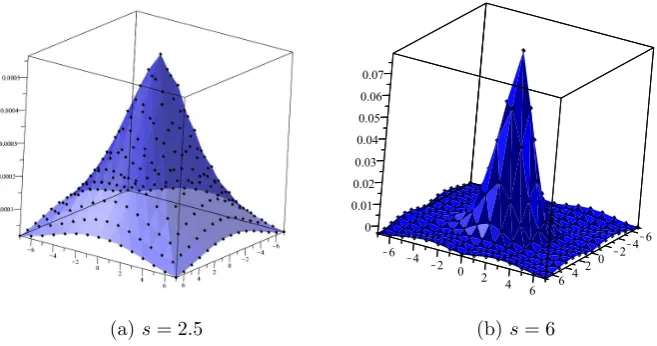
(See Figures 4.2 and 4.3.)
[image:16.595.213.387.340.493.2]Proof. By Proposition 4.5 and Lemma 3.2 the function lM,s satisfies the assump-tions of Lemma 4.6 with h=h1,s andα=s−2 when s∈(2,4) and withh=h2,s and α= 2 when s∈(4,∞). Hence all claims follow from Lemma 4.6.
Figure 4.2. Thes-dependance of α1.
Remark 4.8. Theorem 4.7 shows that the distribution spreads proportionally to
tα1 where α is as in that theorem; cf. [15, Remark 6.2]. When s > 4, one has
normal diffusion since the profile spreads proportionally to t12 in this case. When 2< s <4, however, we observe superdiffusion because then the spread of the profile is proportional totκwithκ=s−12 > 12. In particular, whens= 3, then the profile spreads linearly in time, which is a ballistic behaviour.
One can measure the spread, e.g. with the full width at half maximum (FWHM), which, for our purpose, we can define as
FWHM(t) := 2 sup
r >0 :ux,y(t)≤ 1 2u0,0(t)
for all x, y∈Z with |x|2+|y|2≥r2
.
One can show that FWHM(t)∼ctα1 ast→ ∞with somec >0; cf. [15, Remark 6.2]
(a)s= 2.5 (b)s= 6
Figure 4.3. The graph of the limit solutionFsfrom Theorem 4.7 fors= 2.5 (a) ands= 6 (b), respectively.
Remark 4.9. Let us consider finite truncations of the Mellin transformation (2.6) of thek-path Laplacian, i.e. set
LM,s,N := N
X
k=1 1
ksLk
for N ∈N. By Lemma 3.1 this operator is unitarily equivalent to the operator of
multiplication by the function
lM,s,N(p, q) = N
X
k=1 1
kslk(p, q)
where lk is defined in that lemma. Using Lemmas 4.1 and 4.2 one can show in a similar way as above that
lk(p, q) =2k 3+k
3 (p
2+q2) + O(p4+q4), p, q→0
and hence
lM,s,N(p, q) = N
X
k=1
2k3+k 3ks (p
2+q2) + O(p4+q4), p, q→0.
This leads to normal diffusion by Lemma 4.6 and not to a superdiffusive process like in the non-truncated Mellin transformation. However, the diffusion speed and the variance of the limiting normal distribution grow withN, e.g. if one measures the former with the full width at half maximum, one gets
FWHM(t)∼2 (ln 2) N
X
k=1
2k3+k 3ks
!12
cf. [15, Remark 6.4]. AsN → ∞one has the following behaviour, N
X
k=1
(2k2+ 1)k
3ks ∼ 2 3(4−s)N
4−s, N → ∞, if s∈(2,4),
N
X
k=1
(2k2+ 1)k 3ks →
2ζ(s−3) +ζ(s−1)
3 , N → ∞, if s∈(4,∞).
Whens >4 (i.e. whenuin Theorem 4.7 shows normal diffusion), the coefficient in (4.13) converges to the corresponding coefficient foruasN → ∞, and the limiting normal distributions converge to the limiting distribution from Theorem 4.7. On the other hand, when s∈(2,4), the coefficient in (4.13) diverges as N → ∞. So, although one has normal diffusion for every finite N, the speed of the diffusion — and also the variance of the limiting normal distribution — can be made arbitrarily
large if N is chosen big enough. ♦
References
[1] M. Aidelsburger, M. Atala, S. Nascimb`ene, S. Trotzky, Y. A. Chen and I. Bloch, Experimental realization of strong effective magnetic fields in an optical lattice,Phys. Rev. Lett.107(2011), 255301
[2] E. Akkermans, A. Gero and R. Kaiser, Photon localization and Dicke superradiance in atomic gases,Phys. Rev. Lett.101(2008), 103602
[3] P. Babkevich, V. M. Katukuri, B. F˚ak, S. Rols, T. Fennell, D. Paji´c, H. Tanaka, T. Pardini, R. R. P. Singh, A. Mitrushchenkov and O. V. Yazyev, Magnetic excitations and electronic interactions in Sr2CuTeO6: a spin-1/2 square lattice Heisenberg antiferromagnet,Phys. Rev.
Lett.117(2016), 237203
[4] S. Bahatyrova, R. N. Frese, C. A. Siebert, J. D. Olsen, K. O. van der Werf, R. van Grondelle, R. A. Niederman, P. A. Bullough, C. Otto and C. N. Hunter, The native architecture of a photosynthetic membrane,Nature430(2004), 1058–1062
[5] K. Binder and D. P. Landau, Square lattice gases with two-and three-body interactions: a model for the adsorption of hydrogen on Pd (100),Surf. Sci.108(1981), 503–525
[6] S. Boccaletti, V. Latora, Y. Moreno, M. Chavez and D. U. Hwang, Complex networks: struc-ture and dynamics,Phys. Rep.424(2006), 175–308
[7] G. L. Celardo, F. Borgonovi, M. Merkli, V. I. Tsifrinovich and G. P. Berman, Superradi-ance transition in photosynthetic light-harvesting complexes,J. Phys. Chem. C 116(2012), 22105–22111
[8] G. L. Celardo, G. G. Giusteri and F. Borgonovi, Cooperative robustness to static disorder: superradiance and localization in a nanoscale ring to model light-harvesting systems found in nature,Phys. Rev. B 90(2014), 075113
[9] A. D. C´orcoles, E. Magesan, S. J. Srinivasan, A. W. Cross, M. Steffen, J. M. Gambetta and J. M. Chow, Demonstration of a quantum error detection code using a square lattice of four superconducting qubits,Nature Comm.6(2015), 6979
[10] P. D. Dahlberg, P. C. Ting, S. C. Massey, M. A. Allodi, E. C. Martin, C. N. Hunter and G. S. Engel, Mapping the ultrafast flow of harvested solar energy in living photosynthetic cells,Nature Comm.8(2017), 988
[11] B. Dalla Piazza, M. Mourigal, N. B. Christensen, G. J. Nilsen, P. Tregenna-Piggott, T. G. Per-ring, M. Enderle, D. F. McMorrow, D. A. Ivanov and H. M. Rønnow, Fractional excitations in the square-lattice quantum antiferromagnet,Nature Phys.11(2014), 3172
[12] A. A. Dubkov, B. Spagnolo and V. V. Uchaikin, L´evy flight superdiffusion: an introduction,
Int. J. Bifur. Chaos18(2008), 2649–2672
[13] E. Estrada, Graphs and network theory, In: Mathematical Tools for Physicists. 2nd Edition (editor: M. Grinfeld). John Wiley & Sons, 2013
[14] E. Estrada, J.-C. Delvenne, N. Hatano, J. L. Mateos, R. Metzler, A. P. Riascos and M. T. Schaub, Random multi-hopper model. Super-fast random walks on graphs,J. Compl. Net.6(2018), 382–403
[16] J. F. G´omez-Aguilar, M. Miranda-Hern´andez, M. G. L´opez-L´opez, V. M. Alvarado-Mart´ınez and D. Baleanu, Modeling and simulation of the fractional space-time diffusion equation,
Commun. Nonlinear Sci. Numer. Simul.30(2016), 115–127
[17] J. Grad, G. Hernandez and S. Mukamel, Radiative decay and energy transfer in molecular aggregates: the role of intermolecular dephasing,Phys. Rev. A37(1998), 3835
[18] L. C. Ha, C. L. Hung, X. Zhang, U. Eismann, S. K. Tung and C. Chin, Strongly interacting two-dimensional Bose gases,Phys. Rev. Lett.110(2013), 145302
[19] P. R. Hammar, D. C. Dender, D. H. Reich, A. S. Albrecht and C. P. Landee, Magnetic studies of the two-dimensional,S = 1/2 Heisenberg antiferromagnets (5CAP)2CuCl4 and
(5MAP)2CuCl4,J. Appl. Phys.81(1997), 4615–4617
[20] T. T. Hartley and C. F. Lorenzo, Application of incomplete gamma functions to the initializ-ation of fractional-order systems,J. Comput. Nonlinear Dynam.3(2008), 021103
[21] S. Ji, C. Ates and I. Lesanovsky, Two-dimensional Rydberg gases and the quantum hard-squares model,Phys. Rev. Lett.107(2011), 060406
[22] F. J¨order, K. Zimmermann, A. Rodriguez and A. Buchleitner, Interaction effects on dynamical localization in driven helium,Phys. Rev. Lett.113(2014), 063004
[23] A. A. Kilbas, H. M. Srivastava and J. J. Trujillo, Fractional differential equations: a emergent field in applied and mathematical sciences. In:Factorization, Singular Operators and Related Problems, Kluwer Acad. Publ., Dordrecht, 2003, pp. 151–173
[24] E. Lindel¨of,Le Calcul des R´esidus, Gauthier-Villars, Paris, 1905
[25] X. J. Liu, X. Liu, C. Wu and J. Sinova, Quantum anomalous Hall effect with cold atoms trapped in a square lattice,Phys. Rev. A81(2010), 33622
[26] C. F. Lorenzo and T. T. Hartley, Initialization of fractional-order operators and fractional differential equations,J. Comput. Nonlinear Dynam.3(2008), 021101
[27] J. Lu, J. Shen, J. Cao and J. Kurths, Consensus of networked multi-agent systems with delays and fractional-order dynamics. In: Consensus and Synchronization in Complex Networks, Springer, Berlin–Heidelberg, 2013, pp. 69–110
[28] E. Manousakis, The spin-½Heisenberg antiferromagnet on a square lattice and its application to the cuprous oxides,Rev. Mod. Phys.63(1991), 1
[29] R. Metzler and J. Klafter, The random walk’s guide to anomalous diffusion: a fractional dynamics approach,Phys. Rep.339(2000), 1–77
[30] R. Metzler and J. Klafter, The restaurant at the end of the random walk: recent developments in the description of anomalous transport by fractional dynamics,J. Phys. A37(2004), R161 [31] NIST Handbook of Mathematical Functions, Edited by F. W. J. Olver, D. W. Loizer, R. F. Boisvert and C. W. Clark. U.S. Departament of Comerce, National Institute of Stand-ards and Technology, Washington, DC; Cambridge University Press, Cambridge, 2010. Online verison: http://dlmf.nist.gov
[32] I. Podlubny,Fractional Differential Equations. Academic Press, New York, 1999
[33] U. Schneider, L. Hackerm¨uller, J. P. Ronzheimer, S. Will, S. Braun, T. Best, I. Bloch, E. Demler, S. Mandt, D. Rasch and A. Rosch, Fermionic transport and out-of-equilibrium dynamics in a homogeneous Hubbard model with ultracold atoms,Nature Physics8(2012), 213–218
[34] M. F. Shlesinger, G. M. Zaslavsky and U. Frisch,L´evy Flights and Related Topics in Physics, Proceedings of the International Workshop Held at Nice. Lecture Notes in Physics, vol. 450, Springer, 1995
[35] H. Stahlberg, J. Dubochet, H. Vogel and R. Ghosh, Are the light-harvesting I complexes from Rhodospirillum rubrum arranged around the reaction centre in a square geometry? J. Mol. Biol.282(1998), 819–831
[36] H. Sun, W. Chen, C. Li and Y. Chen, Y., Fractional differential models for anomalous diffusion,Physica A389(2010), 2719–2724
[37] M. M. Valado, C. Simonelli, M. D. Hoogerland, I. Lesanovsky, J. P. Garrahan, E. Arimondo, D. Ciampini and O. Morsch, Experimental observation of controllable kinetic constraints in a cold atomic gas,Phys. Rev. A93(2016), 040701
Department of Mathematics and Statistics, University of Strathclyde, 26 Richmond Street, Glasgow G1 1XH, UK
E-mail address: [email protected]
Department of Mathematics and Statistics, University of Strathclyde, 26 Richmond Street, Glasgow G1 1XH, UK
E-mail address: [email protected]
Department of Mathematics and Statistics, University of Strathclyde, 26 Richmond Street, Glasgow G1 1XH, UK
E-mail address: [email protected]
Institute of Mathematics, L´od´z University of Technology, Ul. W´olcza´nska 215, 90-924 L´od´z, Poland,
Institute of Applied Mathematics and Mechanics, University of Warsaw, Banacha 2, 02-097 Warsaw, Poland
![Figure 4.1. The graph of the functionfor the parameters lM,s on the square [−π, π]2 s = 2.1 (a) and s = 5 (b), respectively](https://thumb-us.123doks.com/thumbv2/123dok_us/1378083.91044/9.595.133.451.120.504/figure-graph-functionfor-parameters-lm-square-p-respectively.webp)