A general framework for combining ecosystem models

Fish and Fisheries. 2018;19:1031–1042. wileyonlinelibrary.com/journal/faf  

|

|

|

DOI: 10.1111/faf.12310

O R I G I N A L A R T I C L E

A general framework for combining ecosystem models

Michael A. Spence

_|

_{Julia L. Blanchard}

_|

_{Axel G. Rossberg}

_|

Michael R. Heath

_|

_{Johanna J. Heymans}

_|

_{Steven Mackinson}

_|

Natalia Serpetti

_|

_{Douglas C. Speirs}

_|

_{Robert B. Thorpe}

_|

_{Paul G. Blackwell}

1_{School of Mathematics and Statistics,} University of Sheffield, Sheffield, UK 2_{Department of Animal and Plant Sciences,} University of Sheffield, Sheffield, UK 3_{Centre for Environment, Fisheries and} Aquaculture Science, Lowestoft, UK 4_{Institute for Marine and Antarctic} Studies and Centre for Marine Socioecology, University of Tasmania, Hobart, Tasmania, Tas., Australia 5_{Aquatic Ecology Group, Department of} Organismal Biology, School of Biological and Chemical Sciences, Queen Mary University of London, London, UK

6_{Department of Mathematics and Statistics,} University of Strathclyde, Glasgow, UK 7_{Scottish Association for Marine}

Science, Scottish Marine Institute, Oban, UK 8_{Scottish Pelagic Fishermen’s Association,} Fraserburgh, UK

Correspondence

Michael A. Spence, Centre for Environment, Fisheries and Aquaculture Science, Pakefield Road, Lowestoft, Suffolk NR33 0HT, UK. Email: [email protected]

Funding information

Natural Environment Research Council and Department for Environment, Food and Rural Affairs, Grant/Award Number: NE/ L003279/1

Abstract

When making predictions about ecosystems, we often have available a number of differ

-ent ecosystem models that attempt to repres-ent their dynamics in a detailed mechanistic

way. Each of these can be used as a simulator of large- scale experiments and make pro

-jections about the fate of ecosystems under different scenarios to support the develop

-ment of appropriate manage-ment strategies. However, structural differences, systematic discrepancies and uncertainties lead to different models giving different predictions. This

is further complicated by the fact that the models may not be run with the same func

-tional groups, spatial structure or time scale. Rather than simply trying to select a “best” model, or taking some weighted average, it is important to exploit the strengths of each of the models, while learning from the differences between them. To achieve this, we

construct a flexible statistical model of the relationships between a collection of mecha

-nistic models and their biases, allowing for structural and parameter uncertainty and for different ways of representing reality. Using this statistical meta- model, we can combine prior beliefs, model estimates and direct observations using Bayesian methods and make coherent predictions of future outcomes under different scenarios with robust measures of uncertainty. In this study, we take a diverse ensemble of existing North Sea ecosystem

models and demonstrate the utility of our framework by applying it to answer the ques

-tion what would have happened to demersal fish if fishing was to stop.

K E Y W O R D S

Bayesian statistics, complex models, multimodel ensemble, multispecies models, simulation models, uncertainty analysis

1 | INTRODUCTION

Ecosystem models are widely used to support policy decisions, in-cluding fisheries and marine environmental policies (Hyder et al., 2015). Any such model is imperfect, and in order to use it to inform policymaking, it is important to quantify the uncertainty of its pre-dictions in a robust manner (Harwood & Stokes, 2003; Williams & Hooten, 2016). Often several models are available, each embodying some knowledge of a given ecosystem, but differing in their predic-tions. Choosing to use one model’s prediction while excluding the

others is limiting the amount of information available and therefore increasing uncertainty. Our aim here is to describe and demonstrate a framework for combining information from multiple ecosystem models in a coherent way that, following Chandler (2013), exploits their strengths and discounts their weaknesses.

Many methods of combining outputs from different models have been previously proposed. One is to use a “democracy” of simulators (Knutti, 2010; Payne et al., 2015), where each model gets one vote, re-gardless of how well it represents the true system, and a distribution of

This is an open access article under the terms of the Creative Commons Attribution License, which permits use, distribution and reproduction in any medium, provided the original work is properly cited.

possible outputs comes from this. Likewise, one could take an average of the model outputs, which often outperforms all the individual models (Rougier, 2016). However, some models are better at predicting some outputs than others. An alternative approach is to try and find the “best” model(s) (Johnson & Omland, 2004; Payne et al., 2015). These methods imply that at least one of the models is “correct,” in the sense that it can predict the true output. Not only is this a bold assumption, but the addi-tion of another model may allow an area of the output space to become probable when before it was not. Thus, by increasing the number of models, there is no guarantee that the uncertainty will reduce. One way of deciding which model is the “best” is to weight models using Bayes factors, also known as Bayesian model averaging (Banner & Higgs, 2017; Ianelli, Holsman, Punt, & Aydin, 2016). As Chandler (2013) explains, there is generally no model better in all respects than the others and so there is no natural way of assigning a single weight to each model. Furthermore, if model outputs are not presented with uncertainty then, in the case where the truth is a continuous quantity, a simulator will almost never be “correct,” and thus, the probability of getting the true value from the ensemble is zero. In recent past, “ensemble models” have been used to describe how model outputs related to reality (Anderson et al., 2017).

Applying the above methods to ecosystem models is not straight-forward, as different models have often been fitted to different data (Ianelli et al., 2016), and often their outputs are on different scales or represent different dynamical processes, which are sometimes in-tegrated out. A further difficulty in applying these methods is that the ecosystem models can have different outputs that are not di-rectly comparable. For example, whole ecosystem models often re-duce complexity through the use of functional groups (Heath, 2012), whereas partial ecosystem or multispecies models may focus on a re-duced number of species (Blanchard et al., 2014). However, different ecosystem models are often developed with similar underlying the-ory (e.g. food web interactions), could have similar dynamics and may even be developed in the same research groups (Heath, 2012; Speirs, Guirey, Gurney, & Heath, 2010). They may also have similar forcing inputs, for example those coming from global regional physical or biogeochemical models such as those used in model intercomparison studies (Tittensor et al., 2017). When combining model outputs, it is important to take these similarities into account rather than treating the models as independent (Rougier, Goldstein, & House, 2013).

Another approach is to think of the ecosystem models as coming from a population of such models (Chandler, 2013; Leith & Chandler, 2010; Tebaldi & Sansó, 2009) and then describe how the population differs from reality. It makes sense that several models in an ensemble model would inform one another. For example, one model (m1) may contain several demersal fish species and the other (m2) a functional group called “demersal fish.” Although m2 does not explicitly contain the species Atlantic cod (Gadus morhua, Gadidae) its relationship with m1 may be able to tell us something about Atlantic cod indirectly. In other words, modelling the models allows us to sample the unob-served outputs, conditional on the models’ obunob-served outputs.

In this study, we describe an ensemble model which is based on the principles of Chandler (2013) but which models the out-puts themselves, varying in form between the different ecosystem

models, rather than statistical descriptors of the outputs. Our ap-proach involves statistical modelling of the relationship between an “ensemble” of ecosystem models. To avoid ambiguity, we will refer to the latter henceforth as “simulators” and we refer to the way in which a simulator output differs from reality as its discrepancy. As we are interested in measuring uncertainty, our statistical model-ling will apply Bayesian inference methods (Robert, 2007), and our analysis will consider any relevant prior knowledge as well as simu-lator outputs that predict what would happen in the future under different management scenarios. The Bayesian approach is sub-jective; for an introduction to subjective uncertainty and decision theory (Berger, 1985). Strictly speaking, any fully Bayesian analysis involves obtaining the posterior beliefs of a particular individual, by combining their prior beliefs with information from data and model-ling. Depending on the context, that individual may be, for example, either a scientist or a policymaker. Our framework includes the elic-itation of prior beliefs to combine with information from the model ensemble, allowing different individuals’ posterior distributions to be obtained. For the purpose of our case study, the individual chosen is one of the authors.

In Section 2, we set up the general framework, and in Section 3, we demonstrate the model by looking at a specific case study: What would have happened in the North Sea if we had stopped fishing in 2014? We conclude by discussing wider applications of the approach in Section 4.

2 

|

 GENER AL FR AMEWORK

We think of the available simulators as coming from some concep-tual population. Our a priori beliefs about each one are the same;

1 INTRODUCTION 1031

2 GENERAL FRAMEWORK 1032

2.1 Uncertainty in simulator outputs 1033

2.2 Individual discrepancy 1034

2.3 Shared discrepancy 1035

2.4 The truth 1035

3 CASE STUDY 1035

3.1 Groups of species 1035

3.2 Data and elements of the statistical model 1036

3.3 Simulators 1036

3.4 Ensemble model 1036

3.5 Results 1037

4 DISCUSSION 1038

4.1 General model features 1039

4.2 Future work and extensions 1040

4.3 Conclusion 1041

ACKNOWLEDGEMENTS 1041

AUTHOR CONTRIBUTION 1041

REFERENCES 1041

we are treating the simulators as unlabelled “black boxes.” More formally, we regard the simulators as “exchangeable” (Gelman et al., 2013). We consider relaxing this assumption in Section 4. This idea is formalized using a hierarchical model (for more infor-mation (Gelman et al., 2013) to represent the ensemble of simula-tors. However, there is no reason to believe that the population of simulators will either contain, or be centred on, the truth (Chandler, 2013), so we need to allow some difference between the population of simulators and the truth.

To describe the relationship between the simulators and the truth, we developed an ensemble model that describes the popula-tion of simulators, its dynamics and its relapopula-tion with the true quantity of interest. We are interested in n true quantities, y(t)_=(y(t)

1,…,y (t)

n)�, for example the biomass of n species at a time t, for times t=1,…,T

. We regard m simulators, each giving an output representing the quantities of interest, x(t)_i =(x(t)

i1,…,x (t)

in)� for i=1,…,m, as coming from a population with expected output 𝝁(t)=(𝜇(t)₁,…,𝜇(t)n)�, the simulator consensus. To define our ensemble model, we describe separately the difference between y(t) _and

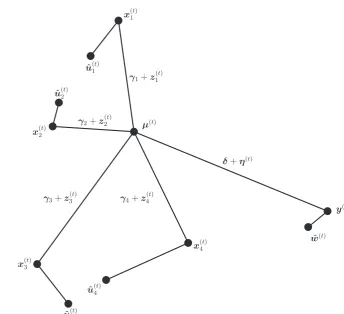
𝝁(t), the shared discrepancy, and the difference between x(t)_i and 𝝁(t), simulator i’s individual discrepancy. Figure 1 illustrates an example of the ensemble model at time t. It can be read as a geometrical representation of how the simulators and reality relate to one another (see also Chandler, 2013). In the subsequent subsections, we describe the specific details of the gen-eral ensemble model. A summary of the variables and the model can be found in Table 1.

2.1 

|

 Uncertainty in simulator outputs

The outputs from simulator i, an ni dimensional vector u

(t)

i , may not always represent the elements of x(t)_i, its “best guess,” directly. For example, the elements of x(t)

i may represent biomasses of individual fish species and the elements of u(t)

i may represent the biomass of functional groups, for example biomass of demersal fish.

We say that

for some simulator- specific function fi(⋅). For example, if the

ele-ments of u(t)

i are elements of x

(t)

i or are sums of those elements, per-haps with some rescaling, then the relationship is linear

where M_i is an n_i×n matrix. For other examples, see Table 2. In general, the simulators are run with uncertain inputs and pa-rameter values. This leads to uncertainty in the outputs and is com-monly known as parameter uncertainty. We say that

for t∈Si, where 𝝐ui has expectation 0 and is sampled from a simulator- specific distribution and û(t)_i is the expectation of the ith simula-tor’s output at time t. The simulator- specific distribution is found from fitting the simulator to a finite data set (Spence, Blackwell, & Blanchard, 2016; Thorpe, Le Quesne, Luxford, Collie, & Jennings, 2015) or by performing sensitivity analysis of the simulator inputs (Morris, Speirs, Cameron, & Heath, 2014).

u(t)_i =f_i(x(t)i ),

u(t)_i =Mix

(t)

i ,

u(t)_i =û(t)_i +𝝐ui,

F I G U R E   1  A schematic that shows an

example of the ensemble model at time t. In this example, we have four simulators that are all able to predict the elements of y(t)_{. Each simulator’s “best guess,” x}(t)

i ,

is observed with parameter uncertainty where û(t)i is the expected output of the ith

simulator (see Section 2.1). The difference between the ith simulator’s “best guess,” x(t)i, and the simulator consensus, 𝝁(t),

is known as simulator i’s individual discrepancy and is split between its long- term, 𝜸i, and short- term, z

(t)

i , individual

discrepancy (see Section 2.2). The difference between the truth, y(t) _{and the} simulator consensus, 𝝁(t), is known as the shared discrepancy and is divided into long- term, δ, and short- term, 𝜼(t), shared discrepancy (see Section 2.3). In addition, we do not directly observe the truth but we do observe a noisy version of it, ŵ(t)

2.2 

|

 Individual discrepancy

At time t, the difference between simulator i’s “best guess,” x(t)_i , and the simulator consensus, 𝝁(t), is simulator i’s individual discrepancy,

This divides the individual discrepancy between the long- term in-dividual discrepancy, 𝜸i, and the short- term individual discrepancy,

z(t)_i. 𝜸_i is an n dimensional random variable with expectation 0 and covariance C. It seems natural to allow z(t)_i and z(t_i+1) to be depend-ent on each other; for example, if at time t, z(t)_i was less than 0, then we might also expect z(t_i+1) to be less than 0. With this in mind, we say that z(t)

i follows a stationary auto- regressive model of order 1,

x(t)_i −𝜇(t)=𝜸i+z

(t)

i

(1) z(t)_i =R_iz(t_i−1)+𝝐z,t,i,

Variable Dimension Times Description Relationship

y(t) _n t = 1 … T The truth _y(t)_=y(t−1)₊

𝝐Λ,t

w(t) _n

y t = 1 … T Possibly incomplete

version of the truth

w(t)_=f y(y(t))

̂

w(t)i ny t∈S0 Noisy observation of w

(t)

̂

w(t)∼p(w_̂(t)|w(t)₎

δ n NA Long- term shared

discrepancy

𝜼(t) n t = 1 … T Short- term shared

discrepancy 𝜼

(t)_=R

𝜂𝜼(t−1)+𝝐𝜂,t

𝝁(t) n t = 1 … T Simulator consensus 𝝁(t)=y(t)₊

𝜹+𝜼(t)

𝜸i n NA Simulator i’s long- term

individual discrepancy

z(it) n t = 1 … T Simulator i’s short- term individual discrepancy z

(t) i =Riz

(t−1) i +𝝐z,t,i

x(it) n t = 1 … T Simulator i’s best guess x

(t)

i =𝝁(t)+𝜸i+z

(t)

i

u(_it) ni t = 1 … T Simulator i’s incomplete version of x(t)

i

u(t)i =fi(x

(t)

i )

̂

u(t)_i ni t∈Si The expectation of

simulator i’s output u(_it)

u(_it)=û(_it)+𝝐ui

TA B L E   1  A summary of the variables in

the ensemble model. The ensemble model is run for t = 1 … T

TA B L E   2  A summary of the simulators, their outputs used in the case study, the simulator- specific function, u(t)

i =fix

(t)

i =Mi10x

(t)

i and a

reference to where the parameter uncertainty, Σi, was calculated

Simulator Description Outputs Mi

Reference for Σi

EcoPath with

EcoSim (EwE) Total biomass is modelled at the species level 1) 2) Common demersalSole

3) Monkfish etc.

4) Sum of Poor cod and Rays and Other

demersal fish

for t = 1991–2023

M1= ⎛ ⎜ ⎜ ⎜ ⎝

1 0 0 0 0 0 1 0 0 0 0 0 1 0 0 0 0 0 1 1 ⎞ ⎟ ⎟ ⎟ ⎠

Mackinson, Platts, Garcia, and Lynam (2018)

mizer Total weight is modelled in

weight classes by species 1) 2) Common demersalSole

for t = 1968–2100

M2= (

1 0 0 0 0 0 1 0 0 0

) _{Spence et al.} (2016)

FishSUMs Abundance in length classes is modelled by species

1) Common demersal

for t = 1990–2098

M3= (1 0 0 0 0) This study, see Supporting information Appendix B StrathE2E Biomass is modelled for

different functional groups

1) Sum of Common demersal, Sole, Monkfish

etc., Poor cod and Rays and Other demersal fish

for t = 1983–2050

M4= (1 1 1 1 1) This study, see Supporting information Appendix B LeMans Abundance in length classes

is modelled by species 1) 2) Common demersalSole

3) Monkfish etc.

4) Poor cod and Rays

for t = 2000–2099

M5= ⎛ ⎜ ⎜ ⎜ ⎝

1 0 0 0 0 0 1 0 0 0 0 0 1 0 0 0 0 0 1 0 ⎞ ⎟ ⎟ ⎟ ⎠

for t>1, where each 𝝐z,t,i is an independent n- dimensional random vari-able centred on 0 with covariance Λi and Ri is an n×n matrix with the constraint such that Ri is stable, that is limk→∞R

k

i=0. Ri and Λi describe the dynamics of simulator i with R_i∼g_R(⋅) and Λi∼gΛ(⋅)} for some

distributions gR and gΛ. At t=1, z

(1)

i is sampled from the stationary dis-tribution of the auto- regressive model described in Equation 2 (See Supporting information Appendix A for more details). This formulation means that the expectation of the long- run behaviour of the individual discrepancy is the long- term individual discrepancy, that is

2.3 

|

 Shared discrepancy

The shared discrepancy, the difference between the simulator con-sensus, 𝝁(t), and truth, y(t), is split up into the long- term shared dis-crepancy, δ, and the short- term shared discrepancy, 𝜼(t), that is

The short- term shared discrepancy is described by a stationary auto- regressive model of order 1

for t>1, where R_𝜂 is stable and 𝝐_𝜂,t is an n dimensional random variable centred on 0 with covariance Δ. At t=1, 𝜼(1) is sampled from the station-ary distribution of the auto- regressive model described in Equation 3 (See Supporting information Appendix A for more details). This for-mulation means that the expectation of the long- run behaviour of the shared discrepancy is the long- term shared discrepancy, that is

2.4 

|

 The truth

In the absence of any simulators, our prior beliefs for the truth at time t, y(t)_{, follow a random walk,}

for t>1, where each 𝝐Λ,t is centred on 0 with covariance Λy. At t=1, the truth, y(1)_{, follows a generic prior distribution p(y}(1)_).

At times t∈S₀, there are n_y noisy and possibly indirect observa-tions, ŵ(t), of the truth which come from some distribution, p(ŵ(t)|y(t)₎ that is problem specific and is caused by data uncertainty (Li & Wu, 2006). The elements of ŵ(t) may not be the same as that of y(t)_{, for} example if observations are incomplete or aggregated. We assume that the sampling distribution of observations depends on the truth through some function f_y(⋅), such that

and p(ŵ(t)|y(t)_)=p(ŵ(t)

|w(t)_).

For example, if w(t) _{is some linear transformation of y}(t)_{, then}

where My is an ny×n matrix.

3 

|

 CASE STUDY

We illustrate our model by looking at a problem where a scientist needs to formally summarize uncertain model results, for example to present to other scientists or to decision- makers about what would happen to the biomass of demersal species in the North Sea if fish-ing were to stop completely in 2014. We use outputs from five eco-system simulators: Ecopath with Ecosim (EwE; Lynam & Mackinson, 2015), mizer (Blanchard et al., 2014), FishSUMs (Speirs et al., 2010), StrathE2E (Heath, Speirs, & Steele, 2014) and LeMans (Thorpe et al., 2015) (see Supporting information Appendix B for more details about the simulators), as well as data from the International Bottom Trawl Survey (IBTS) (ICES Database of Trawl Surveys (DATRAS), 2015). In this example, one of the authors, JLB, has taken this role. Her prior beliefs are elicited and expressed as a prior distribution and the posterior distribution captures her uncertainty about the fu-ture of the ecosystem in this scenario give the relationships among the simulators and observations.

3.1 

|

 Groups of species

The five simulators represent demersal fish in different ways, with different species resolution and coverage. Although our main inter-est is in demersal fish collectively, we need to represent the state of the ecosystem at a resolution that enables us to link these simulator outputs together.

In representing the state of the ecosystem, it would be com-putationally inefficient to treat each species separately, given that we are interested in demersal fish in aggregate. Instead, we can reduce the dimension of the problem by grouping the species to-gether. This grouping needs to have the property that any simula-tor output that we can use can be expressed as the sum of one or more of our groups. The groups do not necessarily need to have any direct biological interpretation, provided the groups meet the criterion above, and allow us to represent the quantities of inter-est—here, demersal fish, given by the sum of all groups—the pre-cise choice will not affect the answer obtained. For computational efficiency, we choose the minimum number of groups that meets this criterion while covering all demersal species. For example, we grouped together monkfish, long rough dab, lemon sole and witch because they all occur in exactly the same simulators, as individual species in EwE and LeMans and implicitly in StrathE2E, but are not contained in any larger set of species for which this is true. This minimal set consists of five groups, which we will model explicitly. The groups are as follows:

limk→∞E(𝜸i+z (t+k)

i |𝜸i+z

(t)

i )=𝜸i+limk→∞E(z (t+k)

i |z

(t)

i ) =𝜸i+E(z

(t)

i ) =𝜸_i.

y(t)₋

𝝁(t)=𝜹+𝜼(t).

(2) 𝜼(t)=R_𝜂𝜼(t−1)+𝝐_𝜂,t,

limk→∞E(𝜹+𝜼(t+k)|𝜹+𝜼(t))=𝜹+limk→∞E(𝜼(t+k)|𝜼(t))

=𝜹+E(𝜼(t)) =𝜹.

y(t)_=y(t−1)₊ 𝝐_Λ,t,

w(t)_=f

y(y(t))

w(t)_=M

1. Common demersal: These are Atlantic cod (Gadus morhua, Gadidae), haddock (Melanogrammus aeglefinus, Gadidae), whiting (Merlangius merlangus, Gadidae), Norway pout (Trisopterus es-markii, Gadidae), European plaice (Pleuronectes platessa, Pleuronectidae), common dab (Limanda limanda, Pleuronectidae) and grey gurnard (Eutrigla gurnardus, Triglidae).

2. Sole: This is common sole (Solea solea, Soleidae).

3. Monkfish etc.: These are monkfish (Lophius piscatorius, Lophiidae), {long rough dab} (Hippoglossoides platessoides, Pleuronectidae), {lemon sole} (Microstomus kitt, Pleuronectidae) and {witch} (Glyptocephalus cynoglossus, Pleuronectidae).

4. Poor Cod and Rays: These are poor cod (Trisopterus minutus, Gadidae), starry rays (Amblyraja radiata, Rajidae) and cuckoo rays (Leucoraja naevus, Rajidae).

5. Other demersal fish: This consists of all other demersal fish.

We consider the total biomass densities for each of these groups, in tonnes per square kilometre, modelled on the log scale (to base 10, for ease of interpretation).

3.2 

|

 Data and elements of the statistical model

The IBTS data were extracted as in Fung, Farnsworth, Reid, and Rossberg (2012), to reveal the total catch on the survey for each of the five groups for the first (1986–2013) and third quarter (1991–2013). How this value relates to the true biomass density in the North Sea is not trivial, and these values are often multi-plied by catchability coefficients (Walker, Maxwell, Le Quesne, & Jennings, 2017), which are themselves uncertain and model- based. In this example, we are only interested in the biomass density rela-tive to 2010, and therefore, the total catch from the IBTS survey is enough provided we assume that catchability coefficients are constant over time. Thus, each element of yt represents the log to base 10 of the total biomass (tonnes per kilometre squared) for one of our groups of species, averaged over year t, relative to 2010. Therefore,

The measurement error on the observations of the truth is assumed to be normally distributed on the log10 scale such that

for t≠2010. In this work, we take Σ_y to be 2 log₁₀(1.15) on the

diago-nal elements and 0 on the off- diagodiago-nal elements. This was chosen so that it means that the standard deviation of the true biomass would be 15% of the actual amount caught.

3.3 

|

 Simulators

We have outputs from five different simulators all of which have been run with zero fishing pressure from 2014 onwards. A short summary of the simulators, their outputs with respect to this case study and their simulator- specific function, f_i(⋅), can be found in Table 2. The ith

simulator’s output is assumed to be normally distributed on the log10 scale,

with Σi fitted based on running simulator i many times (Chandler, 2013; Leith & Chandler, 2010). However, if this was not the case, Σi could be estimated within the hierarchical system.

3.4 

|

 Ensemble model

Each element of x(t)_i is the “best guess” of simulator i of the elements of y(t)_{, for t=1968,…,2100, in log (base 10) tonnes per km squared of wet} biomass. In this example, we expect each of the simulators to converge to its own steady state, given that all external drivers are constant. This means that in Equation 2 we expect R_i to tend towards 1 and Λ_i to tend towards 0. Furthermore, if a simulator reaches a stationary state before it has stopped running, then we know that it will be in that state forever. Simulator i’s individual discrepancy, 𝜸i+z

(t)

i, is thus modelled as

and

where

and

This is saying that, after the end of fishing, the variance of the truth of model i reduces and the amount that the last value of z(t)_i relates to the next moves towards 1 by a factor of exp (ki) each year. We take ki∈[0,6], as there is not much difference numerically if k_i goes above 6, with

The diagonal elements of R_i fall between −1 and 1 with

and the off- diagonal elements are set to 0. The simulator- specific variance parameter, Λi, is decomposed into a diagonal matrix of vari-ances, Πi, and a correlation matrix, Pi, such that

The form of the prior distribution for the jth diagonal element of Πi was

Distributions over correlation matrices are complicated by the math-ematical requirement of positive definiteness. In practice, we specify separate priors on the elements, and then condition on positive defi-niteness; the unconditional prior for the j,kth element of Pi is given by w(t)=fy(y(t))=10y

(t)

.

log10

( ̂

w(t)∕ŵ(2010))∼N(y(t)_,Σ

y),

log10u (t)

i ∼N( log10û (t)

i ,Σi)

𝜸i∼N(0,C)

z(t)_i ∼

{

N(Riz

(t−1)

i ,Λi) if t≤2013, N(h_z(R_i,k_i,t)zt−1

i ,hΛ(t,ki)Λi) if 2014≥t.

h_z(Ri,k,t)=Ri+(1−Ri)(1−hΛ(t,ki))

h_Λ(t,k

i)=exp{−ki

(

t−2013)}.

k_i∕6∼Beta(ak,bk).

R_i+1

2 ∼Beta(aR,bR)

(3) Λ_i= Π_iP_iΠ_i.

𝜋ij∼Gamma(𝛼𝜋,j,𝛽𝜋,j).

𝜌ijk+1

2 ∼

{_Beta(a

𝜌jk,b𝜌jk) ifj≠k,

The difference between the truth at time t and the corresponding simulator consensus, 𝝁(t), is then

with

When the fishing is turned off, we are particularly uncertain about what will happen; thus we will remove any direct relation between yt and yt+1 beyond that time. We will say that

where k_𝜇∈[0,6], so that the simulator consensus reaches a

station-ary point, as the individual simulators do.

We focus on the subjective probabilities of a particular individ-ual, in this case JLB. Her prior beliefs were elicited using the method

described in O’Hagan et al. (2006) and Alhussain and Oakley (2017). Details of the prior elicitation can be found in Supporting informa-tion Appendix C. Due to the dimensionality and correlainforma-tion of the uncertain parameter space, we fitted the model using No U- turn Hamiltonian Monte Carlo (Hoffman & Gelman, 2014) in the package Stan (Gelman, Lee, & Guo, 2015).

3.5 

|

 Results

The ensemble model predictions show changes in the uncertainty of relative biomass over time for each group of species, including projections following a fishing closure in 2014 (Figure 2). Each plot shows the marginal posterior distributions of each element of y(t)_{, for} all t. Unsurprisingly, the ensemble model predicts common

demer-sal fish increase following the fishery closure, as this group contains many species targeted by fisheries.

(

y(t))₋(

𝝁(t)−𝝁(2010)

)

=𝜼(t)+𝜹

(4) 𝜼(t)∼N(R_𝜂𝜼(t−1),Δ_𝜂).

(5) 𝝁(t)∼N(𝝁(t−1),h_Λ(t,k_𝜇)Δ_𝜇)

F I G U R E   2  Estimates of the log biomass of each group of species relative to 2010. The solid line is the median, and the dotted lines are

the upper and lower quartiles. The first vertical line is at 1986, the year that we first have data, and the second line is in 2013, the simulated cessation of fishing

Common demersal

Year

Relati

ve

biomass

1970 1990 2010 2030 2050 2070 2090

0.9

1

1.1

1.2

Sole

Year

Relati

ve

biomass

1970 1990 2010 2030 2050 2070 2090

0.75

1.5

2.5

Monkfish etc.

Year

Relati

ve

biomass

1970 1990 2010 2030 2050 2070 2090

0.5

1

1.5

Poor cod and rays

Year

Relati

ve

biomass

1970 1990 2010 2030 2050 2070 2090

0.5

1

1.5

2.5

4

Other demersal

Year

Relativ

e biomass

1970 1990 2010 2030 2050 2070 2090

0.

51

According to the ensemble model the probability that there will be a greater total biomass of common demersal in 2050 than in 2010 is 0.90. There is a similar number for sole (0.93) and for monkfish etc. (0.88) but it is lower for poor cod and rays (0.55) and for the other demersal species (0.17).

The ensemble model also “predicts” what happened before the data; that is, it gives posterior distributions for the actual val-ues given the imperfect data and the simulator runs. Only sole and common demersal are output by simulators prior to 1986 and this is reflected in the increased uncertainty as we move further back in time from 1986.

The uncertainty in the prediction increases the further away from the observations of the truth, both when projecting and hindcast-ing. The uncertainty also increases when there are fewer simulators that give outputs. All of the simulators give outputs for the common demersal group, four explicitly and one implicitly, and therefore we are more certain about what will happen to it in the future than for poor cod and rays, where only three simulators predict values for the future and only one explicitly. The uncertainty is highest for other de-mersal species. This is understandable as only two simulators predict values for this group of species, neither of which does so explicitly.

The absolute total biomass of demersal species is difficult to calculate here without information on the discrepancy between the simulator consensus and the truth. Although survey data are avail-able, their relationship with the truth depends on the varying, and unknown, catchability coefficients for each of the groups. Although catchabilities can be estimated, for simplicity here we examine the

total demersal biomass under the assumption that the groups had the same catchability coefficients (Figure 3). Again there is high uncertainty about whether the biomass will grow relative to the biomass in 2010. However, what it was before 1986 is also quite uncertain. This is because of the uncertainty in the populations of Other demersal species.

The median “best guess” of each of the simulators can also be compared across the different simulators (Figure 4). StrathE2E pre-dicts quite a large increase in common demersal despite not explicitly outputting it. Mizer does not do a very good job of predicting the dynamics of sole, therefore the dynamics of the simulator consensus do not match the dynamics of mizer.

The posterior predictive distribution for the relative truth in 2025 for common demersal and monkfish etc. are positively correlated with each other (0.28), albeit weakly. This suggests that learning some-thing about the common demersal group would tell you somesome-thing about monkfish etc. Hence the mizer simulator gives some informa-tion regarding the monkfish etc. despite not actually predicting it. See Supporting information Appendix D for the other correlations between the groups.

4 

|

 DISCUSSION

By treating the simulator outputs as coming from a population of simu-lators and modelling this population, we have presented in this study a general way of combining ecosystem simulators to inform scientists

F I G U R E   3  The total biomass of

demersal species as predicted by the models relative to 2010

Total demersal

Year

Relativ

e log biomass

1970 1990 2010 2030 2050 2070 2090

0.

80

.9

1

1.1

and decision- makers about the consequences of management strate-gies. Our model combines many different simulators, exploiting their strengths and discounting their weaknesses (Chandler, 2013) to provide synthetic and comprehensive information to support decision making.

4.1 

|

 General model features

One of the difficulties in building an ensemble model with ecosystem simulators is that the simulator outputs are often done on different scales and are not directly comparable, for example StrathE2E models groups of species (e.g. pelagic, demersal), whereas mizer models major species individually. Our approach, unlike existing methods of combin-ing simulators (e.g. Bayesian model averagcombin-ing (Banner & Higgs, 2017; Ianelli et al., 2016)), allows us to combine outputs from these widely differing simulators. We achieve this by modelling what each simulator would predict for each of the groups of species we are interested in,

whether it is explicitly modelled or not by the simulator. For example, in the case study, StrathE2E only models the total demersal species. Using information from the other simulators regarding the breakdown of de-mersal species and how the dynamics between species work, the en-semble model can say what StrathE2E would predict on a species level. In the case study, EwE and StrathE2E both implicitly predict groups of species. For EwE, it is the sum of poor cod and rays and other demersal, and for StrathE2E, it is the sums of all of the groups. As with the simula-tors that do not predict specific groups, we are able to infer what these simulators predict about implicit groups through correlations learned from other simulators. In this sense, the mizer model, which only pre-dicts common demersal and sole, gives information about how StrathE2E divides its demersal species and therefore gives some information about other groups. Therefore, if we were interested in what would happen to the other demersals if we were to stop fishing, we should include all the simulators despite only two of them predicting it.

F I G U R E   4  The median best guess for the simulators (xi) for mizer (black), FishSUMs (purple), LeMans (green), EwE (red) and StrathE2E

(pink) and the median simulator consensus (𝝁) and its quartiles in solid grey and dotted grey, respectively

Common demersal

Year

Biomass tonnes per km sq

1970 1990 2010 2030 2050 2070 2090

51

02

0

Sole

Year

Biomass tonnes per km sq

1970 1990 2010 2030 2050 2070 2090

0.1

0.2

0.4

Monkfish etc.

Year

Biomass tonnes per km sq

1970 1990 2010 2030 2050 2070 2090

0.25

0.5

1

Poor cod and rays

Year

Biomass tonnes per km sq

1970 1990 2010 2030 2050 2070 2090

0.5

12

4

Other demersal

Year

Biomass tonnes per km sq

1970 1990 2010 2030 2050 2070 2090

0.025

0.1

0.4 Ecopath

Mizer StrathE2E FishSUMs LeMans µ

Simulators that are predictably wrong are more informative than those that are unpredictably wrong, even if the latter are less wrong in the absolute sense. In our framework, we distinguish between short- term and long- term individual discrepancies, which allows us to distinguish between predictably wrong simulators with small short- term individual discrepancies, zi, and unpredictably wrong simulators. Furthermore, we allow the short- term individual discrep-ancies to be different for each group, thus allowing a simulator to contribute to the ensemble model for groups that it is informative about and be ignored for groups that it is not. In the case study, mizer does not predict the dynamics of sole very well and so the simula-tor consensus, 𝝁, only weakly follows the mizer predictions. On the other hand, mizer does a reasonable job of predicting the dynamics of common demersal and therefore it contributes more to the simula -tor consensus for this group. Thus, the ensemble model exploits miz-er’s strengths, common demersal and discounts its weaknesses, sole. The ensemble model enables formal quantification of uncertainty. This uncertainty reflects a specific individual’s updated beliefs having observed the simulators and the observation data (Robert, 2007). The individual could be a scientist or a decision- maker and could be informed by multiple experts (Albert et al., 2012). Such a framework could be used to help communicate uncertainty or enable decision- makers to directly quantify risks and therefore evaluate management trade- offs more rigorously (Finkle, 1990; Harwood & Stokes, 2003). The ensemble model takes account of uncertainty from each of the simulators, through parameter uncertainty and structural uncer-tainty, data unceruncer-tainty, through noisy and possibly indirect observa-tions of the truth, and uncertainty in the ensemble model parameters. As the simulators are describing the same system, we might expect the dynamics in the individual discrepancies to be similar. To reflect this, we allow the short- term individual discrepancies to come from some underlying distribution. Furthermore, in ecosystems simulators, the dynamics may be similar in direction but likely not in magnitude. To include this information in the case study, we split the short- term individual discrepancies, Λi, into correlations and magni-tude (Equation 3), allowing different levels of confidence for each. We used beta distributions for each of the off- diagonal elements of the correlation matrix and then conditioned on positive definiteness. This enabled us to learn about each element of the correlation matrix separately which is not possible in other formulations of the cova-riance matrix (Alvarez, Niemi, & Simpson, 2014). By acknowledging these features of simulators, we were able to better quantify the uncertainty.

It was also important to use informative priors as none of the simulators explicitly model other demersal. As there is no lower bound (on the log scale) for the values of the “best guess” of other demersal, we required some prior information about the distribu -tion of the standard devia-tions, Π. This does suggest that the en-semble prediction is somewhat based on that of the priors for Λi. In practice, we suggest checking that your ensemble model predicts in a way that the decision- maker believes before observing the truth, similar to the hypothetical data method of Kadane, Dickey, Winkler, Smith, and Peters (1980). In the case study described

here, we checked that the dynamics of the biomasses prior to 1986 followed JLB’s beliefs.

When building the ensemble model, how the species groups are decided depends on the question being asked. In the case study, we were interested in what would happen to demersal fish if we were to stop fishing, so we grouped the species into as few groups as possi-ble. However, if we were interested in another question, for exam-ple if we had been interested in what would happen to commercial fish, we would divide the species into groups with commercial and noncommercial fish conditioned on species in each group being pre-sented in exactly the same simulators. As the number of groups in-creases, the dimensions of the covariance matrices increase, so we advise that the number ofgroups be kept to a minimum as this would aid computation time and require less simulators and prior elicitation.

Using the ensemble model developed here, there is no need to identify the ``best model” driven by the question being asked (Dickey- Collas, Payne, Trenkel, & Nash, 2014), but one should in-clude all available simulators. Rather than developing many simu-lation models to answer different specific questions, the ensemble model can be designed to answer the question at hand thus reducing computational costs. Furthermore, as the ensemble model implicitly weights the simulators by their strengths and weaknesses, it is bet-ter for a simulator to be good at modelling one aspect of the ecosys-tem rather than being average at modelling many things (Anderson et al., 2017). Due to tractability it is not possible to explicitly show these weightings in the case study presented here, for an example of weightings in a more tractable example see (Chandler, 2013).

The nature of the different ecosystem simulators capturing dif-ferent processes can limit the number of models available to run certain scenarios (e.g. in climate scenarios where some but not all the simulators contain links to temperature). If we were interested in one of the scenarios that a specific simulator was unable to run, we should still include that simulators in the ensemble model as it gives information about how species interact with one another as well as the state of the ecosystem up until the current time. To include this simulator in the ensemble, we could learn about how it differs from the simulators that were able to run the specific scenario and in-crease a simulator’s parameter uncertainty, Σi, as a function of time with in the future (Szuwalski & Thorson, 2017).

4.2 

|

 Future work and extensions

major source of uncertainty was due to the shared discrepancy, and the results of the ensemble model were close to when all the simula-tors were assumed to be exchangeable.

In this study, we have demonstrated the ideas and methods in cases where the quantities of interest are of fairly low dimension and have joint Gaussian distributions. However, with the increased efficiency of new statistical software and algorithms (Girolami & Calderhead, 2011), it is possible to address larger problems involving more general distributions.

The framework presented here is not exclusive to ecosystem simulators in fisheries, but can be used to combine any mechanis-tic simulators in many areas of ecology (e.g. individual- based models, Railsback & Grimm, 2012) or even other areas of research such as sys-tems biology (Kuepfer, Peter, Sauer, & Stelling, 2007) and epidemiol-ogy (Lessler, Azman, Grabowski, Salje, & Rodriguez- Barraquer, 2016).

4.3 

|

 Conclusion

This work allows for a synthesis of many modelling studies that have been and are being conducted in such a way that we can obtain more holistic knowledge over a wide scope of complex ecological systems. It also allows for including a formal quantitative understanding of uncertainties and knowledge gaps. This enables us to make compre-hensive model projections that take into account all that we have learnt from the simulators collectively.

ACKNOWLEDGEMENTS

The work was supported by the Natural Environment Research Council and Department for Environment, Food and Rural Affairs [grant number NE/L003279/1, Marine Ecosystems Research Programme]. The authors would like to thank Tom Webb, Remi Vergnon, Yuri Artioli, Sévrine Saillery, Paul Somerfield, Melanie Austen, Nicola Beaumont and Stefanie Broszeit for participating in early elicitation exercises. We thank Tony Pitcher and two anony-mous reviewers for comments on an earlier version of the paper.

AUTHOR CONTRIBUTION

MAS, PGB and JLB conceived the ideas and designed the methodol-ogy; JLB extracted the data for the main case study; MAS, MRH, SM, DS, AGR, RBT, JJH and NS ran the simulators for the case study; MAS implemented the methodology; MAS and PGB analysed the data; MAS and PGB led the writing of the manuscript. All authors contrib-uted critically to the drafts and gave final approval for publication.

ORCID

Michael A. Spence http://orcid.org/0000-0002-3445-7979 Julia L. Blanchard http://orcid.org/0000-0003-0532-4824 Axel G. Rossberg http://orcid.org/0000-0001-9014-3176 Michael R. Heath http://orcid.org/0000-0001-6602-3107 Johanna J. Heymans http://orcid.org/0000-0002-7290-8988

Steven Mackinson http://orcid.org/0000-0002-0262-1180 Natalia Serpetti http://orcid.org/0000-0002-9502-5790 Robert B. Thorpe http://orcid.org/0000-0001-8193-6932 Paul G. Blackwell http://orcid.org/0000-0002-3141-4914

REFERENCES

Albert, I., Donnet, S., Guihenneuc-Jouyaux, C., Low-Choy, S., Mengersen, K., & Rousseau, J. (2012). Combining expert opinions in prior elicitation. Bayesian Analysis, 7(3), 503–532. https://doi. org/10.1214/12-BA717

Alhussain, Z. A., & Oakley, J. E. (2017). Eliciting judgements about un

-certain population means and variances. arXiv:170200978. https:// arxiv.org/abs/1702.00978

Alvarez, I., Niemi, J., & Simpson, M. (2014). Bayesian inference for a co

-variance matrix. arXiv:14084050 https://arxiv.org/abs/1408.4050 Anderson, S. C., Cooper, A. B., Jensen, O. P., Minto, C., Thorson, J. T.,

Walsh, J. C., … Selig, E. R. (2017). Improving estimates of population status and trend with superensemble models. Fish and Fisheries, 18, 732–741. https://doi.org/10.1111/faf.12200

Banner, K. M., & Higgs, M. D. (2017). Considerations for assessing model averaging of regression coefficients. Ecological Applications, 27(1), 78–93. https://doi.org/10.1002/eap.1419

Berger, J. O. (1985). Statistical decision theory and bayesian analysis (2nd ed.). New York, NY: Springer Series in Statistics, Springer-Verlag. Blanchard, J. L., Andersen, K. H., Scott, F., Hintzen, N. T., Piet, G., & Jennings, S.

(2014). Evaluating targets and trade- offs among fisheries and conserva

-tion objectives using multispecies size spectrum model. Journal of Applied Ecology, 51(3), 612–662. https://doi.org/10.1111/1365-2664.12238 Blanchard, J. L., Jennings, S., Law, R., Castle, M. D., McCloghrie, P., Rochet,

M. J., & Benoît, E. (2009). How does abundance scale with body size coupled size- structured food webs? Journal of Animal Ecology, 78, 270–280. https://doi.org/10.1111/j.1365-2656.2008.01466.x Chandler, R. E. (2013). Exploiting strength, discounting weakness: Combining in

-formation from multiple climate simulators. Philosophical Transactions of the Royal Society A: Mathematical, Physical and Engineering Sciences, 371(1991), 20120388–20120388. https://doi.org/10.1098/rsta.2012.0388 Demetriou, D. (2016). A Bayesian approach to the interpretation of cli

-mate model ensembles. PhD thesis, University College London. Dickey-Collas, M., Payne, M. R., Trenkel, V. M., & Nash, R. D. M. (2014). Hazard

warning: Model misuse ahead. ICES Journal of Marine Science: Journal du Conseil, 72(8), 2300–2306. https://doi.org/10.1093/icesjms/fst215 Finkle, A. M. (1990). Confronting uncertainty in risk management: A

guide for decision-makers: a report. Tech. rep., Centre for Risk Management, Resources for the Future.

Fung, T., Farnsworth, K. D., Reid, D. G., & Rossberg, A. G. (2012). Recent data suggests no further recovery in North Sea Large Fish Indicator. ICES Journal of Marine Science, 69, 235–239. https://doi.org/10.1093/ icesjms/fsr206

Gelman, A., Carlin, J. B., Stern, H. S., Dunson, D. B., Vehtari, A., & Rubin, D. B. (2013). Bayesian data analysis (3rd ed.). New York, NY: Chapman

and Hall.

Gelman, A., Lee, D., & Guo, J. (2015). Stan: A probabilistic programming

language. Journal of Educational and Behavioural Statistics, 40, 530–

543. https://doi.org/10.3102/1076998615606113

Girolami, M., & Calderhead, B. (2011). Riemann manifold Langevin and Hamiltonian Monte Carlo methods. Journal of Royal Statistical Society, B73, 1–37. https://doi.org/10.1111/j.1467-9868.2010.00765.x Harwood, J., & Stokes, K. (2003). Coping with uncertainty in ecological

advice: Lessons from fisheries. Trends in Ecology and Evolution, 18(12), 617–622. https://doi.org/10.1016/j.tree.2003.08.001

Progress in Oceanography, 102, 42–66. https://doi.org/10.1016/j. pocean.2012.03.004

Heath, M. R., Speirs, D. C., & Steele, J. H. (2014). Understanding pat

-terns and processes in models of trophic cascades. Ecology Letters, 17, 101–114. https://doi.org/10.1111/ele.12200

Hoffman, M. D., & Gelman, A. (2014). The No- U- Turn sampler: Adaptively setting path lengths in Hamiltonian Monte Carlo. Journal of Machine Learning Research, 15, 1593–1623.

Hyder, K., Rossberg, A. G., Allen, J. I., Austen, M. C., Barciela, R. M., Bannister, H. J., … Paterson, D. M. (2015). Making modelling count - increasing the contribution of shelf- seas community and ecosystem models to policy development and management. Marine Policy, 61, 291–302. https://doi.org/10.1016/j.marpol.2015.07.015

Ianelli, J., Holsman, K. K., Punt, A. E., & Aydin, K. (2016). Multi- model infer

-ence for incorporating trophic and climate uncertainty into stock as

-sessments. Deep Sea Research Part II: Topical Studies in Oceanography, 134, 379–389. https://doi.org/10.1016/j.dsr2.2015.04.002 ICES Database of Trawl Surveys (DATRAS) (2015) International Bottom

Trawl Survey (IBTS) data 1985-2014. http://datras.ices.dk.

Johnson, J. B., & Omland, K. S. (2004). Model selection in ecology and evolution. Trends in Ecology & Evolution, 19(2), 101–108. https://doi. org/10.1016/j.tree.2003.10.013

Kadane, J., Dickey, J., Winkler, J., Smith, W., & Peters, S. (1980). Interactive elicitation of opinion for a normal linear- model. Journal of American Statistical Association, 75(372), 845–854. https://doi.org/10.1080/01

621459.1980.10477562

Knutti, R. (2010). The end of model democracy? Climate Change, 102, 395–404. https://doi.org/10.1007/s10584-010-9800-2

Knutti, R., Masson, D., & Gettelman, A. (2013). Climate model geneal

-ogy: Generation CMIP5 and how we got there. Geophysical Research Letters, 40(6), 1194–1199. https://doi.org/10.1002/grl.50256 Kuepfer, L., Peter, M., Sauer, U., & Stelling, J. (2007). Ensemble modeling

for analysis of cell signaling dynamics. Nature Biotechnology, 25(9), 1001–1006. https://doi.org/10.1038/nbt1330

Leith, N. A., & Chandler, R. E. (2010). A framework for inter

-preting climate model outputs. Journal of the Royal Statistical Society: Series C (Applied Statistics), 59(2), 279–296. https://doi. org/10.1111/j.1467-9876.2009.00694.x

Lessler, J., Azman, A. S., Grabowski, M. K., Salje, H., & Rodriguez-Barraquer, I. (2016). Trends in the mechanistic and dynamic modeling of infectious diseases. Current Epidemiology Reports, 3(3), 212–222. https://doi.org/10.1007/s40471-016-0078-4

Li, H., & Wu, J. (2006) Uncertainty analysis in ecological studies. In J. Wu, K. B. Jones, H. Li & O. L. Loucks (Eds.), Scaling and uncertainty analysis in ecology: Methods and applications (pp. 43–64). the Netherlands: Springer. Lynam, C. P., & Mackinson, S. (2015). How will fisheries management

measures contribute towards the attainment of good environmental status for the North Sea ecosystem? Global Ecology and Conservation, 4, 160–175. https://doi.org/10.1016/j.gecco.2015.06.005

Mackinson, S., Platts, M., Garcia, C., & Lynam, C. P. (2018). Evaluating the fishery and ecological consequences of the proposed North Sea multi- annual plan. PLoS One, 13(1), e0190015. https://doi. org/10.1371/journal.pone.0190015

Morris, D. J., Speirs, D. C., Cameron, A. I., & Heath, M. R. (2014). Global sensitivity analysis of an end- to- end marine ecosystem model of the North Sea: Factors affecting the biomass of fish and benthos. Ecological Modelling, 273, 251–263. https://doi.org/10.1016/j.

ecolmodel.2013.11.019

O’Hagan, A., Buck, C. E., Daneshkhah, A., Eiser, J. R., Garthwaite, P. H., Jenkinson, D. J., … Rakow, T. (2006). Uncertain judgements: Eliciting experts’ probabilities. Chichester, UK: John Wiley and Sons.

Payne, M. R., Barange, M., Cheung, W. W. L., MacKenzie, B. R., Batchelder, H. P., Cormon, X., … Paula, J. (2015). Uncertainties in pro

-jecting climate- change impacts in marine ecosystems. ICES Journal

of Marine Science: Journal du Conseil, 73(5), 1272–1282. https://doi. org/10.1093/icesjms/fsv231

Railsback, S. F., & Grimm, V. (2012) Agent-based and individual-based modeling a practical introduction. Princeton, NJ: Princeton University Press.

Robert, C. P. (2007). The Bayesian Choice (2nd ed.). New York, NY: Springer.

Rougier, J. (2016). Ensemble averaging and mean squared error. Journal of Climate, 29(24), 8865–8870. https://doi.org/10.1175/ JCLI-D-16-0012.1

Rougier, J., Goldstein, M., & House, L. (2013). Second- order exchange

-ability analysis for multimodel ensembles. Journal of American Statistical Association, 108(503), 852–863. https://doi.org/10.1080/

01621459.2013.802963

Scott, F., Blanchard, J. L., & Andersen, K. H. (2014). mizer: An R package for multispecies, trait- based and community size spectrum ecolog

-ical modelling. Methods in Ecology and Evolution, 5(10), 1121–1125.

https://doi.org/10.1111/2041-210X.12256

Speirs, D., Guirey, E., Gurney, W., & Heath, M. (2010). A length- structured partial ecosystem model for cod in the north sea. Fisheries Research, 106(3), 474–494. https://doi.org/10.1016/j.fishres.2010.09.023 Spence, M. A., Blackwell, P. G., & Blanchard, J. L. (2016). Parameter un

-certainty of a dynamic multi- species size spectrum model. Canadian Journal of Fisheries and Aquatic Sciences, 73(4), 589–597. https://doi. org/10.1139/cjfas-2015-0022

Szuwalski, C. S., & Thorson, J. T. (2017). Global fishery dynamics are poorly predicted by classical models. Fish and Fisheries, 18(6), 1085– 1095. https://doi.org/10.1111/faf.12226

Tebaldi, C., & Sansó, B. (2009). Joint projections of temperature and precipitation change from multiple climate models: A hierarchical Bayesian approach. Journal of Royal Statistics Society A, 172(1), 83– 106. https://doi.org/10.1111/j.1467-985X.2008.00545.x

Thorpe, R. B., Le Quesne, W. J. F., Luxford, F., Collie, J. S., & Jennings, S. (2015). Evaluation and management implications of uncertainty in a multi- species size- structured model of population and community responses to fishing. Methods in Ecology and Evolution, 6(1), 49–58. https://doi.org/10.1111/2041-210X.12292

Tittensor, D. P., Eddy, T. D., Lotze, H. K., Galbraith, E. D., Cheung, W., Barange, M., … Walker, N. D. (2017). A protocol for the intercom

-parison of marine fishery and ecosystem models: Fish- MIP v1.0. Geoscientific Model Development Discussions, 2017, 1–39. https://doi.

org/10.5194/gmd-2017-209

Walker, N. D., Maxwell, D. L., Le Quesne, W. J. F., & Jennings, S. (2017). Estimating efficiency of survey and commercial trawl gears from comparisons of catch- ratios. ICES Journal of Marine Science, 74(5), 1448–1457. https://doi.org/10.1093/icesjms/fsw250

Williams, P. J., & Hooten, M. B. (2016). Combining statistical inference and decisions in ecology. Ecological Applications, 26(6), 1930–1942. https://doi.org/10.1890/15-1593.1

SUPPORTING INFORMATION

Additional supporting information may be found online in the Supporting Information section at the end of the article.

How to cite this article: Spence MA, Blanchard JL, Rossberg AG, et al. A general framework for combining ecosystem models. Fish Fish. 2018;19:1031–1042. https://doi.