X-ray computed microtomography applications for complex geometries and multiphase flow

(1)

City, University of London Institutional Repository

Citation:

Lorenzi, M. (2017). X-ray computed microtomography applications for complex

geometries and multiphase flow. (Unpublished Doctoral thesis, City, University of London)

This is the accepted version of the paper.

This version of the publication may differ from the final published

version.

Permanent repository link:

http://openaccess.city.ac.uk/19794/

Link to published version:

Copyright and reuse: City Research Online aims to make research

outputs of City, University of London available to a wider audience.

Copyright and Moral Rights remain with the author(s) and/or copyright

holders. URLs from City Research Online may be freely distributed and

linked to.

City Research Online:

http://openaccess.city.ac.uk/

[email protected]

(2)

X-ray computed microtomography applications for

complex geometries and multiphase flow

B.Eng. Massimo Lorenzi

A thesis submitted for the fulfilment of the requirements of City,

University of London for the degree of Doctor of Philosophy

CITY, UNIVERSITY OF LONDON

School of Mathematics, Computer Science & Engineering

(3)

(4)

TABLE

OF

LIST OF ILLUSTRATIONS

Figure 1-1 (Top) localization of X-ray wavelengths and energies, distinguished as soft and hard X-rays, in

the electromagnetic spectrum; (Bottom - from left to right) application of X-rays to determine the

arrangement of atoms in the crystalline solids, breast cancer screening radiography, head and neck

computed tomography scan, airport security baggage scanning for safety reasons. [38] ... 32

Figure 1-2 Schematic section view of a transmission target X-ray source. From left to right we can find the

filament cathode (in red), the produced beam of electrons (in green), the alignment unit and focusing

electronic lenses (in orange), the electron target (in grey), the output window (in purple) and the mitted

X-ray beam (in yellow). ... 32

Figure 1-3 Visualization of the production of X-rays through the interaction of electrons with target atoms.

Electrons numbered 1 to 4 hit the target from left producing X-rays of energy proportional to the intensity

of their interaction with the nucleus and its electrons. Image inspired by an illustration present in [37]... 32

Figure 1-4 Image of the electrons travelling inside the target material produced with software “CASINO”

[39]. ... 33

Figure 1-5 Tungsten (W) target spectrum simulated with Spektr software [40]. ... 33

Figure 1-6 Contribution of each X-ray attenuation mechanism calculated for Beryllium and X-rays energies

between 5 keV and 160 keV with software XMuDat [41] based on tabulated values of [42]... 36

Figure 1-7 Representation of the interaction between an incoming monochromatic X-ray radiation and a

homogenous object material. ... 36

Figure 1-8 X-ray CMOS detector simplified layout. From left to right: incoming X-ray radiation, protection

plate (grey), scintillator layer (yellow), fibre optic plate (blue), photodiode (green), CMOS sensor (purple)

and electronic readout circuitry (orange). ... 39

Figure 1-9 Conversion probability of Caesium iodide phosphor doped with Thallium based on incoming

X-ray energies form 0 to 120 keV. Source: redrawn from [43]. ... 39

Figure 1-10 Image from (Gdh-commonswiki) First prototype of computed tomography scanner produced

by Sir Godfrey Newbold Hounsfield and Allan MacLeod Cormack. In the left image Sir. Hounsfield is

pictured with his first commercially available CAT, in the right picture the CAT prototype is visible with a

sample brain as object to be scanned. ... 41

Figure 1-11 Layout of sample tomographic acquisition. From left to right we have the X-ray source,

represented with a pointwise emission, the rotary stage with the cubic object to be scanned positioned on a

sustaining cylindrical sample holder, the detector where the transmitted radiation is acquired and sampled

to be saved in a 2D image file, the stack of acquired radiographies, one for each positional step, ready to be

processed for reconstruction ... 41

Figure 1-12 Illustration of the object shape and position guess through projections observation: the volume

(7)

projections shown on the right it is clearly impossible to guess the correct shape and position of the two

objects even though each projection furnish partial data about the desired information. ... 41

Figure 1-13 Schematic view of the circular cone beam tomography with mid-plane highlighted. Image from

[45] ... 42

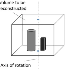
Figure 1-14 Graphical visualization of the rotation axis of the selected volume to be reconstructed. ... 42

Figure 1-15 (from top left to bottom right) original projection image without corrections; dark, gain and

defect image to be used for projection correction; image corrected with the previous three correction

images; legitimized and normalized image; cosine weighted image; ramp filtered image; smoothed image;

horizontal and vertical slices resulting from the reconstructed injection channel ... 44

Figure 1-16 Sinogram of the proposed sample reconstruction of a cylinder and a parallelepiped. (Right)

three sample projections are displayed corresponding to angle 0°, 90° and 135°. (Middle) line profiles of

the same detector line extracted for all the three projections. (Right) complete sinogram from 0° to 360° of

the analysed line before image logarithmisation and filtration. ... 44

Figure 1-17 Left: unfiltered sinogram (top) and simplified back projection of a point (bottom) showing the

image blurring that would results by the back-projection process if the images weren’t high-pass filtered.

Right: same sinogram image ramp filtered to enhance high frequencies (top) and same back projection of

a point with filtered sinogram. It is clear the necessity of the filter enhancing high frequencies. ... 45

Figure 1-18 Back projection process: each projection line is back projected on the projection plane, which

represents an horizontal cross section plane of the reconstructed volume, to reconstruct by summation the

shape and material property value of the scanned object. ... 45

Figure 1-19 Outside view of the X-ray machine with door open; control electrical cabinet on the right side

of the picture. ... 47

Figure 1-20 Close-up view of the inside of the cabinet with (from right to left) X-ray source, rotary stage

and X-ray detector displayed. ... 47

Figure 1-21 Coordinate system of the microCT machine. ... 47

Figure 1-22 Emission axis alignment process: one radiography at each specific distance from the X-ray

source is acquired and processed to obtain the emission centre as perceived by the detector. Based on this

information the overall emission axis can be calculated and corrected moving the detector if not linear. . 48

Figure 1-23 Left – colour coded radiography of the non -aligned X-ray source: the X-ray intensity is not

symmetric with respect to the detectors’ centre point. Right – same colour coded radiography of the same

X-ray source after alignment: X-rays intensity symmetry is evident. ... 48

Figure 1-24 (left) schematic view of microCT setup evidencing distances of interest for magnification

calculation; (right) penumbra phenomenon illustrated: (right-top) a perfect nominally pointwise X-ray

source projects a single X-ray emission cone creating a sharp single image of the object on the detector

panel, while (right - bottom) an X-ray source with non-negligible dimension produces a penumbra effect

(8)

only for the first face of the cube object and for just one side (worst case) of the emitting area, side 1, the

same happens symmetrically for emission point 2. ... 50

Figure 1-25 Air bearing rotary stage produced by Aerotech utilized to rotate the sample during radiographies acquisitions. ... 50

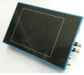
Figure 1-26 X-ray detector utilized to acquire X-ray images during tomographies. The front surface shows the carbon fibre window that seals and protects the active scintillator area. On the side the BNC trigger in and trigger out connectors are visible. On the same size the power supply connector and the Ethernet cable plug are present. ... 51

Figure 1-27 Modulation transfer function as communicated by the detector producer ... 52

Figure 1-28 Linearity of the detector over its full range scale. ... 52

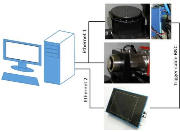
Figure 1-29 Illustration of the control equipment layout of the tomography machine. ... 53

Figure 1-30 (Left) nano-bar phantom positioned near to a match for scale comparison. (right) enlarged view of the middle section of the phantom cylinder revealing the inside with the two chips positioned axially (chip1) and perpendicularly (chip2). Source: image courtesy of QRM GmbH (with own overlays) ... 56

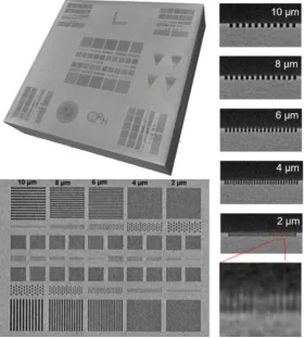
Figure 1-31 : (left) layout of the full engraved area of the two silicon chips contained in the phantom. (right) zoom of the central part of the engraved area showing line and point patterns with width from 10 to 1 µm. Source: image courtesy of QRM GmbH ... 56

Figure 1-32 (left) Slanted edge present on the QRD phantom. (right) indication of the portion of the slanted edge utilized for the calculation of reconstruction resolution. ... 56

Figure 1-33 (top-left) 3D rendering of the reconstructed volume of the vertical chip of the QRM phantom. (bottom-left) Zoom of the central area of the phantom where it is clearly visible the possibility to distinguish lines of 4 µm with the nominal tomography resolution set at 2.19 µm.(right) from top to bottom cross cut of the 10-8-6-4-2 µm lines to show engraved lines distinguishability down to 4 µm, while the 2 µm apart lines are not clearly identifiable. ... 57

Figure 1-34 Plot of the Modulation Transfer Function (MTF) for the area selected on the reconstructed phantom slice. ... 57

Figure 1-35 Zoom of the plot of the Modulation Transfer Function (MTF) for the right hand side of the modulation transfer function of the edge with indication of the function values for 10% transmission. .. 58

Figure 1-36 Plot of the Edge Spread Function (ESF) for the area selected on the reconstructed phantom slice. ... 58

Figure 1-37 Plot of the Line Spread Function (LSF) for the area selected on the reconstructed phantom slice. ... 58

(9)

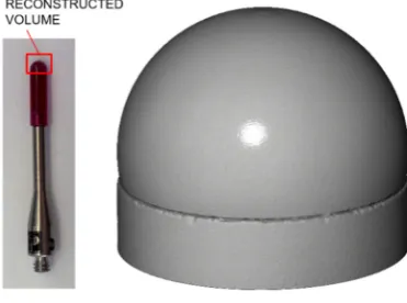
Figure 1-39 (left) picture of 2 mm Renishaw stylus with (right) its rendered reconstruction form CT data.

... 59

Figure 1-40 (left) in red reconstructed stl surface points selected for the fitting operation. (right) in green

nominal fitted sphere overlaid to the original reconstructed stl surface shown in grey. ... 60

Figure 1-41 Table of deviation from nominal sphere of mesh reconstructed from microCT data considering

a 3 sigma Gaussian fitting of original sphere surface points. ... 60

all available points of original sphere surface. ... 61

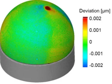
Figure 1-43 Deviation of sphere surface created with all available points to show pole artefact. As it can be

seen the mesh deviation points that increase by three times the surface deviation from nominal spherical

geometry are concentrated near the tomography rotation axis (dark brown in the figure). ... 61

Figure 1-44 (left) in red stl surface cylinder points selected for the calculation of the fitting nominal

cylinder. (right) in green nominal cylinder created form the selected pints overlaid to the original stl surface

shown in grey. ... 61

Figure 1-45 Table of deviation from nominal cylinder of mesh reconstructed from microCT data

considering 3-sigma points of original surface. ... 62

Figure 1-46 (left) overall and zoomed picture of 0.3 mm Renishaw stylus and (right) its rendered

reconstruction from CT data. ... 62

Figure 1-47 (left) in red selected surface point to fit nominal geometry (right) nominal sphere (in green)

created with the fitting operation overlaid to the original mesh (grey). ... 63

3-sigma points of original surface. ... 63

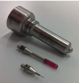
Figure 1-49 (From top to bottom) picture of the diesel injector tip that will be the object of geometrical

reconstruction within this thesis, and the 2 mm and 0.3 mm Renishaw styli to visualize the scale between

the three objects. ... 63

Figure 1-50 (right) schematic section view of the reference scaling phantom created with the two Renishaw

styli: the outer plexiglass container has been cut to reveal the layout of the two styli. (left) picture of the

real sample produced and utilized... 64

Figure 1-51 (left) stl surface of the two styli reconstructed from the single CT dataset. (right) in green

3-sigma fitting spheres utilized to calculate the distance between the centres, the line connecting the two

centres is highlighted as “reference distance”. ... 65

Figure 1-52 (left) axially perpendicular slice of a sample metal cylinder showing beam artefact in the form

of degrading greyscale values in the direction going from the outer border to the cylinder centre. (right)

plot of greyscale values vs. diameter position of the yellow line over imposed to the cylinder section present

(10)

Figure 1-53 (left) axially perpendicular slice of a Diesel injector tip reconstructed with microCT showing

streaks artefacts produced by injection holes, yellow arrows highlight modification of calculated attenuation

value which is visible for areas inside the injector material and outside (air). (centre) plot of greyscale values

indicated by the line in the left image, blue arrows show lower attenuation due to beam hardening streaks.

(right) same slice after beam hardening correction application,... 66

Figure 1-54 Unfiltered (grey line) versus filtered (blue) spectrum. ... 66

Figure 1-55 (left) radiography of the step wedge created with a tack of metal foil of 0.4 mm thickness and

(right) grayscale values plot of the yellow line through its length. ... 67

Figure 1-56 (left) radiography of Diesel injector tip without needle with yellow line over imposed to the

area utilized for the calculation of the self-wedge map. (right) Illustration of the thicknesses calculation for

the object of interest. ... 68

Figure 1-57 (left) plot of the greyscale value of the radiography indicated by the yellow line showing

detected material attenuation through material thickness. (right) table of radiography greyscale values vs

position to be used to correlated greyscale valued with calculated thicknesses. ... 68

Figure 1-58 (left) same axially perpendicular slice of the sample metal cylinder showing beam artefact

correction result. (right) plot of greyscale values vs diameter position of the yellow line over imposed to

the cylinder section present in the left image revealing grey values homogeneity improvement due to

applied correction. ... 69

Figure 2-1 a) A diagram that shows the contact angle and interphase-energy between 3 phases (gas, liquid,

solid). b) drop triple line highlighted in red. Images from a) [68] b) own. ... 72

Figure 2-2 Section view of the ideally axisymmetric drop visualizing the two radii utilized by the

Laplace-Young equation. ... 73

Figure 2-3 A droplet resting on a solid surface and surrounded by a gas forms a characteristic contact angle

θ. If the solid surface is rough, and the liquid is in intimate contact with the solid asperities, the droplet is

in the Wenzel state. If the liquid rests on the tops of the asperities, it is in the Cassie-Baxter state. Image

from [78] ... 73

Figure 2-4 Drop of distilled water of almost 5 mm diameter gently deposed on a Teflon surface. ... 76

Figure 2-5 Level with a resolution of 50 micrometre per meter utilized for the drop on Teflon. ... 76

Figure 2-6 a) Drop of distilled water on Teflon cylinder (picture taken with a discarded cylinder. b) Sample

radiography of the surface with deposed drop. ... 76

Figure 2-7 Visualization of the drop on Teflon positioned in front of the X-ray source for scanning purposes.

The partially anti-evaporation cap and beneath water pool is visible... 76

Figure 2-8 a) superposition of reference drop radiographies (before and after tomographic acquisition in

the same position). b) zoomed view of the drop contours showing the still present evaporation effect. ... 77

Figure 2-9 Overlay of drop radiography before and after tomographic scan without anti-evaporation cap.

(11)

Figure 2-10 Top-left – reconstructed volume section showing attenuation coefficient difference between

drop and Teflon. Bottom-left – coloured render with transparency of the reconstructed drop-surface volume.

Right – solid 3D render of the reconstructed volume. ... 78

Figure 2-11 top left – stl drop surface visualized in green with radial sections shown in black. top right –

visualization of only the radial sections contours (36 of the 120 used). Bottom left and right – top and

bottom view of the drop-surface stl clearly showing the non-circular footprint of the drop. ... 79

Figure 2-12 Reprinted with permissions from [79]. 3D rendering of the fitted profiles coloured to represent

experimental-fitted profiles deviation. Colour from blue (0%) to red (3.85%) is proportional to the

dimensionless error ∆R/Rmax ... 79 Figure 2-13 a) – b) Reprinted with permissions from [79]. Graphical visualizations of the triple line

trajectory and contact angle measurement comparison between experimental and fitted datasets. a) xy plane

localized comparison of drop-surface points: green circles represent experimental points while black circles

represent fitted data, the maximum distance between analogous points is 72 µm b) contact angle

measurements: green dots represent positions where experimental and fitted contact angle measurements

are in good agreement, 192 points of the original 240, while red triangles represent point with bad

agreement... 79

Figure 2-14 top-left – sample drop deposed on the record surface. Top-right schematic section of the record

profile to highlight characteristic geometrical measures (p = 320 µm; h = 92 µm; w = 136 µm). bottom-left,

bottom-right: side view of a sample surface-drop couple. ... 81

Figure 2-15 Picture of a small drop of Glycerol on top of the needle utilized to place it on the patterned

surface. ... 82

Figure 2-16 Left – section of drop reconstructed volume before application of radiation filtering: the two

yellow arrows highlight the position of the artefact caused by the beam hardening showing in the section

as a wide horizontal line of pixels with non-correct grey level values. The image has been smoothed to try

to minimize via software the detected defect in the first instance. Right – section of a comparable drop

reconstructed volume produced after the introduction of the aluminium filter, it can be noted that the beam

hardening is diminished. ... 82

Figure 2-17 left – angled side view of the reconstructed vinyl record surface showing the groves sides

irregularities that produce music when hit by a turntable needle. The yellow arrow highlights the

tomography rotation axis artefact. Right – top view of the same record surface. ... 83

Figure 2-18 Two side views (top-middle) and a three-quarter view (bottom) of the biggest drop no.5

artificially positioned near to the smallest one no.2 to highlight the difference of drops volume. ... 83

Figure 2-19 Top left – rendering of drop 1 tomographic reconstruction. Top right – conversion of

reconstructed drop-surface volume in STL format after separate identification of drop and surface volume.

Bottom left – in yellow recognized footprint of the drop. Bottom right – visualization of the only drop

(12)

Figure 2-20 1st_{row-left – drop and surface stl surfaces ¾ view. 1}st_{row, right - only drop stl surface displayed}

in red with numbered sections (black lines) produced by planes perpendicular to the grooves. 2nd_row-left:

semi-transparent drop visualization to reveal contours of drop surface sections 1 to 4. 2nd_{row right –}

orthogonal view of section 1 (blue) and 4 (red) to reveal the pinning behaviour change: section 1 is

characterized by strong left-right side symmetry, while section 4, corresponding to the central section of

the drop, is highly non-symmetric since the left side of the drop overspills the edge of the groove while the

right side doesn’t. 3rd_{and 4}th_{row: orthogonal display of section 1 to 4 with indication of left-right drop}

contact angle with difference highlighting the non-symmetric behaviour of the drop-surface pinning ... 85

Figure 2-21 1st_{row left: drop and surface stl surfaces ¾ view. 1}st_{row right: only drop stl surface displayed}

in red with numbered sections (black lines) produced by planes parallel to the grooves. 2nd_row-left:

semi-transparent drop visualization to reveal contours of drop surface sections 1 to 4. 2nd_{row right – orthogonal}

view of section 1 (blue) and 4 (red) to reveal the symmetry in the pinning behaviour. 3rd_{and 4}th_row:

orthogonal display of section 1 to 4 with indication of left-right drop contact angle with difference

highlighting the symmetric behaviour of the drop-surface pinning. ... 86

Figure 2-22 Visualization of 3D drop base area extraction (yellow) and its projection on surface parallel

plane to calculate the 2D footprint of the drop. ... 88

Figure 2-23 top row: 3D drops footprints on the record surface. Bottom row: 2D projection of the only

drops footprints. ... 88

Figure 2-24 black line presents nominal surface Wenzel roughness ratio calculated utilizing the nominal

geometry of the record surface, while the single points present the experimental results for the 4 drops of

interest. I can be noted that the latter are in good agreement with the theoretical corresponding value.

However, the experimental points referring to drop n.2 and n.3, which have very similar volume, are quite

distant one form the other, this can be explained with the different way of covering the surface edges of the

two drops, which is not represented by the single nominal value. Image from [85] ... 88

Figure 2-25 left – 6 x 7 mm size GDL carbon cloth utilized for the tomographic reconstruction presented;

single carbon fibres can have a diameter range between 5 and 10 µm. right – same piece of carbon cloth

with a drop of distilled water deposed. ... 91

Figure 2-26 Top – 3/4 view of the GDL reconstructed volume, yellow section at sides represents recognized

fibre volume: as it can be seen, inside strands, single carbon fibres are merged in one bigger volume. Bottom

– higher zoom top view of a small portion of the GDL to further highlight the visibility of some of the

carbon fibres protruding from the strands. ... 91

Figure 2-27 Grayscale rendering of thresholding window utilized to determine the only drop volume. It is

clearly visible that under the drop, the GDL volume is partially visualized meaning that it will be recognized

as drop volume after thresholding operation. ... 91

Figure 2-28 Left - rendering of the tomographic results of GDL with DROP (top) and only GDL (bottom)

(13)

Figure 2-29 Left (top) – side view of the drop volume after thresholding and GDL subtraction. Left (bottom)

tilted view of the same drop volume. Right – bottom view of the drop volume showing regularly spaced

grooves, determined by the warp and weft surface of the GDL cloth ... 93

Figure 2-30 Top row left: rendering of the reconstructed drop volume. Top row right: visualization of the

portion of the drop surface which is inside the GDL. Bottom row, from right to left: visualization of the

drop sections as the section plane considered enters the GDL cloth. The remaining drop volume calculated

after each section drop volume cut is: 0.951 mm3_{, 0.294 mm}3_{and 0.026 mm}3_{. ... 93}

Figure 2-31 Top-left: in blue 3D rendering of the drop surface with radial sections overlapped in black and

red, 18 items in total, one section each 10°. Top-right – visualization of the only drop profiles to reveal the

complexity of drop surface footprint. Bottom-left: orthogonal view of red single drop profile present in the

previous images. Bottom-right: B-spline drop contour profiling and contact angle measurement of red drop

profile presented in the previous images. ... 93

Figure 2-32 From top left to bottom right – tilted view of drop surface sectioned by 6 planes parallel to the

GDL surface to show how the drop adapts to the detected surface defect. The sectioning planes are the same

utilized in the previous figure. ... 94

Figure 2-33 From top left to bottom right – top view of drop surface sectioned by 6 planes parallel to the

GDL surface to show how the drop adapts to the detected surface defect. ... 95

Figure 2-34 Visualization of tomographic reconstruction slices highlighting drop pinning in more than one

position. The full slice is visible in the left while in the right the zoomed view of the area where the pinning

occurs is zoomed to ease details detectability. ... 95

Figure 3-1 Top left: closeup view of injector nozzle placed inside the microCT machine ready to be scanned.

The nozzle has been disassembled from the body and the needle has been removed to place the nozzle on

top of the sample holder. Top right: complete view of injector nozzle inside the microCT machine. The

nozzle distance from the X-ray source allows a magnification which produces a tomography with a 4 µm

resolution. ... 98

Figure 3-2 Left – CAD drawing of the top mounting sample holder. The only tolerance indicated is the h7

for the base diameter since this must tightly match the diameter of the hollow rotary stage central hole. The

tolerance for the top hole where the nozzle sits is not indicated since the nozzle outside shape is conical.

... 98

Figure 3-3 Top left – radiography of the nozzle produced with the reported settings. Top right – false

coloured radiographic image showing in false colours the intensity of the radiation received by the X-ray

detector. Bottom row – schematic view of the tomography set-up to identify the position of the metal filter

utilized to filter the incoming radiation. ... 100

Figure 3-4 Left column, top and middle – nozzle reconstructed slices (horizontal and vertical) without beam

hardening correction applied - Right columns, top and middle - same nozzle slices presented in the left part

of the figure but with beam hardening correction applied. Bottom, left – histogram of the reconstructed

(14)

in the reconstructed volume. Bottom, right – histogram of the reconstructed volume with beam hardening

correction applied, showing two main peaks corresponding to air (peak no.2) and nozzle metal material

(peak no.4). Peak no. 2 is still present highlighting that not all the beam hardening artefact has been

cancelled out by the correction. ... 100

Figure 3-5 Top – thresholding of non-beam hardening corrected nozzle slice: yellow line represents the

nozzle area recognized contour. The injection holes’ exit is not reconstructed correctly since the pixel value

in this position have a higher grayscale value which assigns them to the nozzle material instead that to air

as supposed. Bottom – same slice with beam hardening correction; the brighter pixel values of the outer

border have been corrected permitting detection of the hole geometry. ... 101

Figure 3-6 Top, left – histogram of the nozzle tomography showing selected threshold value corresponding

to the min histogram value between material peaks. Top, right – same histogram presented in the left image

but with air and nozzle histogram values assigned colour coded. Bottom – nozzle slice colour coded using

threshold value. ... 101

Figure 3-7 3D rendering, drawing and picture of DIN bushing utilised for the dimensional checks. ... 103

Figure 3-8 Measurement of the DIN guide bushing with the Mitutoyo micrometre. ... 103

Figure 3-9 Left – 3D rendering of the DIN guide bushing sub-volume reconstructed by microCT. Middle –

picture of the real part with reconstructed sub-volume identified by the black square. Right – stl

reconstructed surface of inner and outer cylinders utilized for the diameter size calculations: “D” indicates

the inner diameter while “d” indicates the outer diameter size. ... 103

Figure 3-10 Top left – nominal CAD design geometry for the internal volume of the studied nozzle. Top

right – reconstructed geometry produced by microCT data. Bottom – over position of CAD and CT

geometries with the CT surface colour coded to reflect surface to surface distance. ... 104

Figure 3-11 Top left – tilted bottom view of the reconstructed nozzle geometry with highlight of the position

of the defect detected. Top right – zoomed view of the same geometry presented in the left to better reveal

the defect. Bottom left – defect presented with deviation colouring exceeding used scale. Bottom right –

picture of the defect produced after cutting the injector in half to reveal the inside. ... 105

Figure 3-12 Left column – zoomed pictures of the nozzle to locate the nozzle part that will be in the

reconstructed volume at the three level of resolution. Right column – radiographies from the tomographic

datasets at the three chosen resolution levels. ... 105

Figure 3-13 Left – 60-degree sector cutting operation inside microEDM machine, the nozzle is being cut

by the metal wire which constitutes the eroding electrode; the actual erosion point is visible on the tip of

the nozzle as a blue point representing the electrode spark position. Right – 60-degree nozzle tip sector after

erosion placed on a fingertip. ... 107

Figure 3-14 Left column – from top to bottom 3D renderings of the reconstructed volumes with three

different reconstruction resolutions (4.665 µm, 1.950 µm, 0.927 µm). Right column – from top to bottom

(15)

Figure 3-15 Top left – 3D rendering of nozzle tip with geometry section visualized. Top right – orthogonal

view of channel cross section with numbers indicating the measured dimensions. Bottom left – cross cut

view of the nominal CAD geometry. Bottom right – close up of inlet rounding of the nominal CAD channel

geometry. ... 108

Figure 3-16 Plot of inlet/exit up/down rounding radii (mean values). Tomographic resolution of points is

colour coded as per the legend presented in the right part of the image. ... 109

Figure 3-17 Left - Inlet and exit diameters (mean values) for the different tomographic resolution utilised.

Bottom, right – mean channel length value for the three tomographic resolution ... 110

Figure 3-18 Top left - SEM image of the full nozzle tip. Top right – SEM measurement of the EXIT

diameter of one injection hole. Bottom left – Tilted view of the same injection hole exit to reveal channel

roughness caused by microEDM machining. The darker region with a ring shape around the channel exit

has not been studied further. Bottom right – zoomed view of exit edge of channel. ... 111

Figure 3-19 Left – external view of 3D CAD model. Centre – section view of CAD model showing internal

injection channel position and geometry. Right – zoomed orthogonal view of only injection channel with

needle added visualizing flow path and asymmetric needle utilised... 112

Figure 3-20 Left column from top to bottom – surface geometry of injection channel after running-in

reconstructed with microCT; nominal injection channel cylinder; microCT geometry coloured to represent

geometrical deviation of reconstructed surface from nominal cylindrical feature. ... 112

Figure 3-21 Shadowgraphy of injection channel showing cavitation as dark area; the flow direction is from

left to right and the injection channel is displayed horizontally. Images from top to bottom display three

testing conditions with increasing cavitation presence. ... 114

Figure 3-22 From top to bottom orthogonal views of the 4 sides of the injection channel presenting

geometrical deviation of channel geometry reconstructed after usage versus same channel geometry

acquired before usage. ... 114

Figure 4-1 Left – 3D CAD image of the test rig as available for the high-speed visualizations. Right, top –

Picture of the same rig assembled and utilized: the area surrounded by the red dashed line highlights the rig

horizontally mounted on the optical table. Right, bottom – close up CAD and picture of the test chamber,

the CAD image presents the hypothetical rotation axis mentioned. ... 117

Figure 4-2 Left - 3D CAD image of the test rig as designed and produced for the X-ray tomographic

reconstructions. Centre – Picture of the test rig placed inside the microCT machine. Right, top – middle

cross section of the test chamber CAD to reveal the inside, the rotation axis or the rig is coincident with the

injection channel one. Right, bottom, picture of the new test chamber. ... 117

Figure 4-3 Left – Fem analysis of the PEEK test chamber model produced to assess geometrical

deformation induced by maximum pressures (100 bar upstream the injection channel and 20 bar

downstream). Centre – X-ray radiography of composite materials analysed for X-ray penetrability. Right –

(16)

Figure 4-4 Top-left – Section of 3D CAD model showing inner injection channel geometry, sealing O-rings

and fixing clamps position. Top-right: 2D CAD drawing of the sample model presenting a section of it

showing its design dimensions. Bottom – 2D CAD drawing of the non-symmetric needle. ... 120

Figure 4-5 Left – microCT customized test rig parts description and localization. Right – Layout of the

hydraulic circuit utilised to provide pressurized fluid for the experiment and to monitor interesting

experimental conditions. ... 121

Figure 4-6 Left, top – Peek disk with the 3 mm non-through hole in the middle. Left, bottom – same Peek

disk in front of the X-ray source, the back disk of the same dimensions on top of the Peek disk, the brighter

one, is carbon fibre reinforced Peek material which was not selected due to its lower X-ray transparency.

Right – radiography, mean of one hundred radiographies, of only the hole area with a drop of diesel inside,

numbers present the projected attenuation through the sample as perceived by the detector. ... 123

Figure 4-7 Left – 3D tomographic reconstruction of the central part of the sample, sectioned with a middle

plane to reveal the inside. Here a drop of diesel is present. Right – orthogonal view of section presenting

reconstructed values for air and diesel to assess the possibility to differentiate liquid diesel and diesel

vapour, which was considered for simplicity of equal attenuation as air. ... 123

Figure 4-8 Plot of simulated Tungsten (W) target emission spectrum determined by an X-ray source voltage

of 130 kV. Plot produced with software Spektr 3.0 [40]. Characteristic peaks are indicated by text and added

blue lines. ... 126

Figure 4-9 Simulated plot generated with Spektr presenting the X-ray spectrum produced by an X-ray

source voltage of 60 kV. The absence of the higher Tungsten characteristic peaks is evident, while the lower

energies peaks are filtered out by the detector lower energy detection threshold. ... 126

Figure 4-10 Left – Simulated X-ray spectra for an X-ray source voltage set of 60 kV, red line presents

generated spectrum as exiting from the X-ray source while blue line presents same spectrum after filtration.

Right – zoomed view of the filtered spectrum to better show its quasi Gaussian shape and resulting mean

energy. ... 126

Figure 4-11 Left – Cross section of visualization test chamber with square recollecting volume. Right –

Cross section of microCT test chamber with conical and afterwards cylindrical recollecting volume. ... 127

Figure 4-12 Shadowgraphy set-up presenting the components mentioned in the text: light source, focussing

lenses, test chamber model and high-speed camera. ... 128

Figure 4-13 Left- schematic view of test injection channel. Right – from top to bottom three shadowgraphy

images are obtained with same needle lift equal to 1 mm in different conditions... 128

Figure 4-14 (top-left) projection of empty channel and (top-right) projection of channel full of Diesel.

(Bottom-left) reconstructed slice of empty channel showing attenuation difference, by means of different

grayscale values, between surrounding PEEK material and void channel. (Bottom-right) reconstructed slice

of channel full of Diesel liquid. ... 130

Figure 4-15 (left) axially cut 3D representation of the injection channel of interest with cavitation

(17)

the axis revealed. (right) Same slice of the reconstructed volume shown flat to reveal ring artefacts and

shape of cavitation which is also circular in shape. ... 130

Figure 4-16 (top left) sample slice of liquid reference dataset. (top right) sample slice of air reference

dataset. (middle -left) sample slice of 10 percent void dataset before calibration: the probability density

function plot of the values inside the channel border, indicated in the image by a yellow circle, is visible on

the right of the image. (bottom left) Same sample slice of 10 percent void dataset after calibration and only

visual contrast enhancement. ... 131

Figure 4-17 Illustration of the mixing procedure followed to create 10 to 90 percent void fraction reference

datasets for scale linearity check. The projections have been mixed interlacing them in order to obtain an

even effect of the modification proposed, better simulating cavitation presence and absence behaviour.

... 131

Figure 4-18 Void fraction calibration scale with 1-sigma bars ... 133

Figure 4-19 Void fraction calibration scale with 3-sigma bars ... 133

Figure 4-20 Visual representation of the created calibration scale: it can be noted that vapour fractions

which are farther from the reference calibration dataset with 0 and 1 void fraction present more uncertainty.

... 134

Figure 4-21 Top: high speed shadowgraphy picture of experimental conditions of experiment no.2. Middle:

and bottom: Calculated mean and standard deviation images. ... 136

Figure 4-22 Top – Vertical plane integration of the calculated void fractions multiplied by pixel dimension

to retrieve a void fraction thickness in the direction perpendicular to the integration plane. Middle -overlay

of the shadowgraphy mean image displayed in Figure 4-21 with the contour of the area presenting more

than 25 µm of vapour thickness in the previous image. Bottom – same overlay presented before but with

the standard deviation image instead of the mean image. All images refer to experiment no. 2. ... 136

Figure 4-23 Top-left: 3D rendering of the injection channel volume reconstructed by microCT with liquid

fraction rendered transparent. Top-right: Front view of the channel entrance. Bottom cross cut view of the

injection channel with shadows to reveal three dimensionalities of the cavitation structures. All images refer

to experiment no.2. ... 137

Figure 4-24 Top: shadowgraphy picture revealing the string like vortex between the needle tip and the

channel entrance. Middle: standard deviation image revealing the localization of the string like vortexes.

Bottom: cross cut view of microCT reconstructed volume presenting cavitation structures which may be

connected to the presence of string like vortexes detected by the shadowgraphy images. All images refer to

experiment no. 2. ... 138

Figure 4-25 (1 of 2) Top: cross cut view of the MicroCT injection channel reconstructed volume presenting

a red line every 600 µm. Following numbered images: sections perpendicular to the channel axis produced

in the positions located by the previously mentioned red lines. All images refer to experiment no.2. ... 140

(18)

Figure 4-27 Single shot sample shadowgraphy pictures for all experiments ... 145

Figure 4-28 Calculated mean image for each experimental shadowgraphy dataset. ... 146

Figure 4-29 Calculated standard deviation from the mean image for each experimental shadowgraphy dataset... 147

Figure 4-30 3D rendering, front channel view and axial sections for experiment no. 3... 148

(19)

(20)

LIST OF TABLES

Table 6-1 Specification of the utilized glycerol. ... 80

Table 6-2 Table summarizing the characteristics of the drops ... 82

Table 7-1 Extended description of the names utilized in Figure 7-14 ... 108

Table 7-2 Average value and correlated standard deviation for measurements of injection channels features

introduced in Figure 7-15. ... 109

Table 8-1 Range of experimental conditions. ... 121

Table 8-2 Diesel physical and chemical properties (as specified by the producer). ... 122

Table 8-3 Table of mean and variance values calculated for the non-calibrated and calibrated 10 percent

void case (100 slices). ... 130

Table 8-4 Statistical values calculated for the experimental data after fitting with normal distribution. . 132

(21)

(22)

ACKNOWLEDGMENTS

Firstly, I would like to thank Prof. Manolis Gavaises for starting and making all this research adventure

possible through trust and financial support. Secondly, Prof. Maurizio Santini for failing at the beginning

to convince me not to embark in such an adventure, having therefore to host me in his laboratory and

granting me access to his equipment for all the coming research period, and more. Thirdly, to a true

experimental researcher, Dr. Nicholas Mitroglou, for showing me true passion for research.

In addition, I want to thank my wife, born under the stars of hope, love and strength, she uses all her qualities

with me every day, and my two sons, Leonardo and Nicola, true shining stars came to planet earth during

(23)

(24)

DECLARATION TO THE UNIVERSITY LIBRARIAN

I hereby declare that the work presented in this thesis is my own and was developed in a joint effort with

other members of the research group of fluid dynamics of City, University of London, led by Prof. Manolis

Gavaises, and the research group of thermodynamics, laboratory of microtomography, of the University of

Bergamo, led by Prof. Maurizio Santini.

I grant powers of discretion to the University Librarian to allow this thesis to be copied in whole or in part

without further reference to me.

This permission covers only single copies made for study purposes, subject to normal conditions of

acknowledgement.

London, 24/12/2017 Faithfully,

__________________________

(25)

(26)

THESIS ABSTRACT

In all fields, fundamental and applied research seek to produce experimental measurements without causing interferences to the process being observed. This capability is of paramount importance, since small perturbations of the phenomenon can alter it to the point of producing biased or even incorrect results. X-ray techniques, based on synchrotron or laboratory X-X-ray sources, have attracted the attention of the research and industrial R&D community thanks to their characteristic of having little to no detectable influence on the subject under study. Moreover, if declined as tomography, this technique can provide localized full volume information at the micrometre scale, from which arbitrary shaped geometries and material densities can be deduced.

During this thesis an X-ray microtomography instrument, based on a laboratory X-ray source, has been exploited to gain three main objectives.

The first one is the analysis of how a liquid drop, of water or glycol, adapts its shape to reach an equilibrium state when gently deposed on a flat or patterned surface. So far this has been done using 2D techniques but introducing the knowledge of the third dimension and being able to see the drop shape even in not optically accessible locations, opens new possibilities to better understand the physics that regulate it.

The second one is the reconstruction of the internal geometries of automotive diesel injectors with high resolution to detect and highlight differences between nominal and real geometries, key information to produce more realistic CFD simulations of the flow inside production grade injectors geometries. A scaled -up model made of PEEK was also studied, producing successive tomographies, to detect small geometrical changes induced by part usage, giving an in-depth view of the locations more prone to be damaged by cavitation flow.

(27)

(28)

THESIS INTRODUCTION

The present research has been conceived to advance the knowledge of possible usage of micro computed

tomography (microCT) to study complex geometries and multiphase flows. The custom build equipment

utilised for this scope was already designed and in use before the start of the present research, however

applicability of X-ray tomography and of the mentioned instrument to the study of the following research

subjects was desired to be assessed.

1. Analysis of liquid-surface interaction.

Knowledge of how a liquid drop wets its resting surface is used to predict performances of processes driven

by this characteristic in many engineering fields such as:

-

heat exchangers [1]

-

lubrication of moving parts [2]

-

gas and crude oil extraction from soil [3]

or study how chemical and mechanical artificial modification of surfaces can produce desired surface

characteristics:

-

functional surface coatings [4]

-

functional surface patterning [5]-[7]

Traditionally the understanding of such an interaction was obtained studying the solid-liquid characteristic

contact angle, which implies the measurement of the angle between the drop profile and the surface, to

deduce the hydrophobic or hydrophilic behaviour of the surface with regards to the used liquid. Techniques

such as the telescope-goniometer, the captive bubble method, the tilting plate, the Wilhelmy balance, the

pendant drop [8], the immersed plate [9] and the sessile drop method [10] are used.

However, techniques as the reported ones, which are based on the optical acquisition and analysis of drop

side views, suffer from drawbacks due to optical lenses aberration, which causes image blurriness and

distortion, need of high illumination, which can induce liquid evaporation, and light diffraction at drop

surface contact line which produces non-usable pictures. Another drawback of traditional techniques is

their impossibility to measure the proposed contact angle for patterned or irregular surfaces where the point

of contact between the liquid and the drop is not directly visible.

For regularly patterned surfaces, more modern techniques such as reflection interference contrast

microscopy [11], [12] or laser scanning confocal microscopy [13] can produce contact angle measurements

but they need transparent surfaces patterned with specific parallel grooves through which they are able to

directly visualize the drop-surface contact line.

This research work aims at assessing the possibility to use microCT for the determination of the liquid-drop

(29)

To obtain the stated scope, new dedicated experimental set-ups will be created to test microCT technique

to analyze liquid-surface interaction in the case of surfaces that are:

-

flat

-

regularly patterned

-

random shaped.

Obtained results with the new proposed method, that was conceived by the research group after the advice

of Prof. G.E. Cossali and B. Weigand, will be compared to similar analysis produced with more traditional

techniques where possible.

This research subject will be developed in:

Chapter 2: Applications to complex geometries – (thermal-fluid dynamics).

2. Micrometric scale reconstructions of diesel injectors internal geometries for accurate CFD

simulations.

The fuel injection process is very actively studied in the will of controlling engine performances, reduce

pollutant emission and improve engine’s durability [14].

Traditionally CFD simulations have been paired with direct experimental tests to gather the necessary data

to improve the design of fuel injectors. However, producing experimental data consumes time and materials

which could be partially spared if CFD simulation trustworthy could be improved [15], [16].

Traditionally simulation is performed using as boundary domains CAD reconstructions of nominal injectors

internal geometries, however this is known to be inaccurate, especially for simulation of flows with

cavitation presence, due to differences that are always present between nominal geometries and real

geometries which can be accounted to production tolerances. Moreover, modern injection geometries

characterised by injection holes with diameters in the order of 150-200 µm pose severe technological

difficulties in their production which can threaten even more production stability of key geometrical

characteristics [17], [18] In the will of knowing the true internal geometry of injection nozzles without the

will to use destructive testing, techniques such as silicon moulding [19], [20] and direct tactile

measurements [21] have been utilised. However, silicon moulding poses significant difficulties in

extracting the mould for complex geometries and its intrinsic elasticity raises doubts on its possibility to

accurately copy the objects’ true dimensions, while direct tactile measurement has the necessity to directly

access to the point of measurement. The most promising non-destructive high resolution technique to

retrieve the nozzle internal geometry is X-ray tomography which is able to reconstruct its full 3D volume

with micrometric resolution, in the range of 3-10 µm, implying the usage of synchrotron X-ray sources

[22], [23] or laboratory X-ray sources [24]. This research work aims at testing the possibility to use the

available new custom laboratory micro-focus X-ray source to reconstruct with a resolution as high as 1 µm

the internal geometry of production grade diesel injectors with injection holes of 150-200 µm diameter and

non-cylindrical holes so to be able to create in the future a dataset of real injector geometries that can be

(30)

To obtain the stated scope, tests will be first performed to define a specific acquisition set up for automotive

diesel injectors and a dedicated reconstruction procedure to reduce the influence of known X-ray

microtomography artefacts [25]. Then reconstructions of internal nozzle geometries with resolutions

increasing to as much as 1 µm will be performed and compared to similar information obtained with

traditional measuring methods (SEM images and direct tactile instruments) to test the capabilities of the

available microtomographic machine.

Chapter 3: Applications to complex geometries (real injectors + test rig model)

3. Quantitative measurement of void fraction distribution inside fuel injection channel.

Diesel flowing inside injectors nozzles is prone to cavitate due to localized de-pressurization of liquid

imposed by nominal operating conditions, small orifice dimensions and sharp flow path deviations [26].

Cavitation can be beneficial, it can improve spray atomization [27], [28], or detrimental, reduces discharge

coefficient, modifies spray angle and liquid length penetration, promotes localized nozzle erosion [14].

Traditionally visualization techniques such as shadowgraphy, Schlieren and interferometry have been

employed to study cavitation in transparent nozzle replicas, made of plastic or even quartz material,

presenting transparent injection channels with direct optical access.

Used nozzle dimensions can vary from real ones to enlarged ones, scaled up 10x to 15x, to improve sample

production feasibility and ease experimental conditions through the reduction of injection pressures. Results

produced employing enlarged models replicate with a good degree of confidence results observable for real

size nozzles thanks to the dimensionless similarity that can be imposed to the flow selecting equal cavitation

(C.N.) and Reynolds numbers [29]-[31].

However, the opacity of cavitation structures to visible light doesn’t allow gathering shape and density

information about their core, particularly in case of strong cavitation, imposing the selection of an

alternative technique to obtain the desired knowledge. X-ray can be used to penetrate opaque materials

thanks to their characteristic wavelengths, permitting to retrieve sample density information leveraging the

well-established relation between sample X-ray absorption and its density.

X-ray radiography and tomography are the two main techniques that can be used to see through even dense

cavitation structures, collecting information about the density of their structures. In case of radiography,

density information will represent the summed up projected sample density along the X-ray path: this

technique has been recently used employing a laboratory X-ray source to study two dimensional cavitating

flows obtaining a two-dimensional map void fraction values [32]. In case X-ray tomography is employed,

the sample density information will be three dimensionally localized.

Synchrotron X-ray sources have been utilised to study cavitation inside injection nozzles [33], [34],

however, due to the limited access to this kind of equipment and the small time slot that can be allocated

for a single research, first attempts to use purposely designed laboratory X-ray sources instead of

synchrotron light sources are being made such as [35]. This latter work has inspired the work presented in

(31)

This research work aims at using X-ray tomography to produce three-dimensional quantitative void fraction

values distribution maps through experimental data acquisition and analysis which can be used to advance

knowledge of cavitation structures dependence on flow properties and injection geometry.

To obtain the stated scope the following steps will be performed:

-

Design of a test rig chamber specifically tailored to produce experimental data applying X-ray tomographic technique with interchangeable sample injection geometries. The first sample

geometry will be designed taking inspiration by the geometry presented in [36].

-

Acquire experimental data to characterize different flow conditions.

-

Analyse the obtained experimental data to quantitatively measure the mean flow density in the full 3D volume of the injection channel determining localized void fractions values.

Chapter 4: Applications to multiphase flow – cavitation.

The first chapter of this thesis (Chapter 1- Description of microCT technique and equipment) will introduce X-ray tomographic technique and the utilised instrument to present the techniques and method along with

(32)

1 DESCRIPTION OF MICROCT TECHNIQUE

AND EQUIPMENT

1.1 INTERACTION OF X-RAYS WITH MATTER.

Electromagnetic radiation with a wavelength between 0.01 and 10 nanometres is termed X-rays. The name

to this kind of photons was implicitly given by Wilhelm Conrad Röentgen who accidentally discovered

them in 1896: not knowing the nature of the radiation he was detecting, he decided to call it simply “X”,

which stands for unknown. Figure 1-1 shows the position of the X-ray radiation in the electromagnetic

spectrum and the vast number of applications permitted by its usage. Different X-rays wavelengths

correspond to different photon energies, that can go from around 1 keV (kilo electron Volt) to 10 MeV [37].

For laboratory X-ray sources like the one used for this thesis, the production process of X-rays starts in the

X-ray source where in a vacuum chamber a heated metallic filament produces free electrons by thermionic

effect. The produced electrons are then captured and accelerated in the direction of a metallic target from

the presence of a voltage differential, in the order of tenths to hundreds of kilovolts, between the heated

filament, which represents the electronically negatively charged cathode of the electronic circuit, and a thin

metallic plate which represents the anode. During the travel between the cathode and the anode, the electron

beam is focused by a single, or sometimes double, stage of electronic lenses: this equipment reduces the

dimension of the cross section of the beam by focusing it on a very small area of a metallic target, of the

order of micrometres in diameter as shown in Figure 1-2. The interaction of the electron beam with the

target atoms produces X-rays through energy conversion. When the negative charge of an electron interacts

with the positive charge of the atom’s nucleus due to their vicinity, its speed is reduced, resulting mainly

in the bending effect on its trajectory. This speed reduction, which is called Bremsstrahlung effect, meaning

“breaking” in German language, is proportional to the distance between the electron trajectory and the

atom’s nucleus position. As it is represented in Figure 1-3 by the case of electrons 2-3-4, different

interaction distances make the electron lose different quantities of energy which are converted in X-rays of

corresponding wavelengths. The Bremsstrahlung effect can produce X-rays of any energy up to the

maximum energy of the electrons of the electron beam, value which is controlled by the X-ray source

voltage set. Besides the mentioned breaking effect, X-rays are also produced by incoming electrons

impinging directly on the atom’s electrons: their collision can cause the atom’s electron to be ejected and

substituted by an electron coming from an outer shell. The jump of the atom’s electron from a higher

energy orbital to a lower energy one, forces the electron to lose energy which is converted in an X-ray of a

specific wavelength. Since the energy released by this kind of interaction is peculiar to the energies of the

orbitals of the target material, it is called characteristic radiation, case of electron 1 in the image above.

It must be however underlined that only around 1% of the electrons’ energy is transformed in X-rays, the

remaining 99% is destined to heat up the target, creating important target heat dissipation problems due to

the high energy density. To have an idea of how much strongly electrons’ trajectories are diverted due to

(33)

Figure 1-1 (Top) localization of X-ray wavelengths and energies, distinguished as soft and hard X-rays, in the electromagnetic

spectrum; (Bottom - from left to right) application of X-rays to determine the arrangement of atoms in the crystalline solids,

breast cancer screening radiography, head and neck computed tomography scan, airport security baggage scanning for safety

reasons. [38]

Figure 1-2 Schematic section view of a transmission target X-ray source. From left to right we can find the filament cathode

(in red), the produced beam of electrons (in green), the alignment unit and focusing electronic lenses (in orange), the electron

target (in grey), the output window (in purple) and the mitted X-ray beam (in yellow).

Figure 1-3 Visualization of the production of X-rays through the interaction of electrons with target atoms. Electrons

numbered 1 to 4 hit the target from left producing X-rays of energy proportional to the intensity of their interaction with the

(34)

[image:34.595.184.470.52.301.2]

Figure 1-4 Image of the electrons travelling inside the target material produced with software “CASINO” [39].

Figure 1-5 Tungsten (W) target spectrum simulated with Spektr software [40].

Figure 1-4 depicts a side view of the trajectories of 1,000 electrons, simulating an electron beam of 1

micrometre diameter, produced by a nominal X-ray source set at 120 keV, hitting a metal target plate of 5

x 5 micrometre and 2 micrometre thickness made of tungsten (W). The plate is represented in grey with

50% transparency to let the inner trajectories of the electrons to be seen; the false colour of the trajectories

represents the decreasing of the electrons energies as it is lost while interacting with the target and being

diverted.The Bremsstrahlung effect produces X-rays of many different wavelengths that constitute the

continuous part of the emitted X-ray spectrum, the other part is given by the characteristic radiation

mentioned before. Figure 1-5 represents a simulated spectrum of X-rays produced by a tungsten (W)

metallic target when hit by an electron beam produced by an X-ray source set at a voltage between cathode

and anode of 120 kV: the characteristic radiation is visible as peaks at 59.31 keV and 67.23 keV over

imposed to the continuous radiation produced by the Bremsstrahlung effect. In the same image, it is evident

(35)

electron, in the case of a complete electron stop. The most of X-rays produced have an energy of about 1/3

of the maximum electron energy and for the proposed sample spectrum the mean photon energy can be

calculated to be 55.73 keV.

In the case of a transmission target like the one described, which is only two micrometres thick, a window

made of a low X-ray attenuating material such as Beryllium (Be) is necessary to contrast the mechanical

forces applied by the presence of the high vacuum inside the ionizing chamber of the X-ray source and to

filter the secondary electrons ejected from the target atom shells. The produced X-rays pass through this

material before reaching open air and be available for use.

The quantity of X-rays that reaches the object is governed by the inverse square law, since the target

material area where the rays are produced can be in the first instance considered as a pointwise source, with

divergent X-rays emission and, similarly to light, linear propagation.

The initial intensity (I0), as well as fluence, of the X-rays diminishes while moving away from the electron

target following the inverse square law:

=

Equation 1-1

Where represents the intensity of the beam at a distance from the source.

When the X-rays produced meet an object along their path, target window as previously said and air

included, they can interact with it with a probability that depends on:

- X-rays initial energy.

- Material’s atomic number.

- Material’s density.

- Travelled distance inside the material (material thickness).

The result of the X-rays travel through the object can be either an absorption, a trajectory deviation

(scattering), or a non-interaction.

In the energy range produced by laboratory sources, such as the one used for this thesis, from 5 keV to 160

keV, the X-ray interaction mechanisms are the:

- Photoelectric effect

The X-ray photon transfers its total energy to a shell electron of the object material, mainly of the inner

shells, ejecting it and forcing another atom’s electron of an outer shell to fill the void, releasing energy as

electromagnetic radiation of a specific wavelength with unknown direction. The ejected electron is called

photoelectron and can contribute to further ionization processes.

The photoelectric effect is more present when the energy of the incoming X-rays is near to the binding

energy of the atom’s electron to be ejected.

(36)

Equation 1-2

Where is the target material atomic number, its density and the energy of the incoming electrons. As it can be seen, even a small difference in material atomic number , causes the effect to increase by a large amount.

- Compton effect (incoherent/inelastic scattering)

X-ray photons transfers only partially their energy to a shell electron of the object material, mainly of the

outer shells, ejecting it. The photon on the other hand lose part of its energy and deviates its trajectory from

the original one. The ejected electron can further ionize electrons of other atoms. The decreased energy of

the photon causes also the wavelength of the radiation to become longer, changing its material penetrability.

The Compton scattering effect is more presents for atoms with high electron density and therefore for high

material density objects, while it reduces with incoming radiation energy.

This kind of attenuation effect does not depend on the target material atomic number.

- Rayleigh effect (coherent/elastic/Thomson/classic scattering)

X-ray photons trajectories are deviated by the presence of the target material atoms, considered, but with

no loss of energy since the interaction between the photon and the atom is not strong enough to reach the

minimum energy necessary to eject an atom’s electron. This scattering effect is dependent on the atomic

number of the target material as follows:

Equation 1-3

Figure 1-6 presents the contribution of each attenuation mechanism described to the total X-rays attenuation

for the energies of interest of laboratory X-ray sources. On the x-axis X-ray energies between 5 keV and

160 keV are displayed, while the y-axis presents the mass attenuation coefficient tabulated for the specific

material selected, Beryllium.

The presented interaction mechanisms produce an attenuation of the incoming X-rays intensity which is

exponential and proportional to the thickness of the passed through material as represented by Figure 1-7.

If we consider the simplest case of a monochromatic radiation and an object made of a homogenous

material, the following formula describes the attenuation of X-rays:

d = − d

(37)

Figure 1-6 Contribution of each X-ray attenuation mechanism calculated for Beryllium and X-rays energies between 5 keV

and 160 keV with software XMuDat [41] based on tabulated values of [42]

Figure 1-7 Representation of the interaction between an incoming monochromatic X-ray radiation and a homogenous object

material.

Where is the number of incoming photons, is the linear attenuation coefficient, and x is the thickness of the passed through material. X-rays that are not attenuated continue to travel on their initial trajectory

after passing through the object material. The solution of the proposed differential equation (2) is:

= 0

Equation 1-5

Which is more commonly used in the following form where the number of photons is referred to as X-ray

intensity:

=