Covariance Symmetries Detection in PolInSAR Data
Sofiane Tahraoui , Carmine Clemente ,
Member, IEEE
, Luca Pallotta ,
Member, IEEE
,
John J. Soraghan,
Senior Member, IEEE
, and Mounira Ouarzeddine
Abstract— In the last two decades, the use of synthetic aper-ture radar (SAR) for remote sensing purposes has significantly developed due to improvements in the quality and the avail-ability of the images. Two powerful SAR techniques, namely, polarimetry and interferometry, have further increased the range of applications of the sensed data. Using polarimetry, geometrical properties and geophysical parameters, such as shape, roughness, texture, and moisture content, can be retrieved with considerable accuracy, while interferometric information may be used to extract vertical information with accuracy less than 1 cm. In this paper, the potential of using joint polarimetry and interferometry techniques in SAR data (PolInSAR) for the purpose of SAR image classification is investigated. To achieve this goal, we extend a covariance symmetry detection framework to the PolInSAR sce-nario. The proposed approach will be shown to be able to exploit the peculiar structures of the covariance matrices of PolInSAR images to discriminate structures within the image. Results using real-SAR data are presented to validate the effectiveness of the proposed approach.
Index Terms— Azimuth symmetry, cross covariance, detec-tion, polarimetric interferometry, PolInSAR, reflection symmetry, rotation symmetry, symmetries.
I. INTRODUCTION
P
OLARIMETRIC interferometry is a recent technique, [1] which uses two spatially shifted polarimetric antennas allowing the measurement of the coherence associated with the various polarimetric channels as well as the height of the polarimetric phase centers. The potential of this technique for the extraction of physical parameters from vegetation, ice, and urban areas has been validated on various data sets and is still being evaluated on other types of data acquired at high resolu-tion by airborne systems [2]–[4]. The polarimetric scattering phenomenon of a medium can be described completely using a (3×3) matrix formulation, namely, the covariance matrix [5]. In general, the medium encountered exhibits symmetric prop-erties, for example, the forest canopy layer, which consists of randomly oriented leaves twigs and branches, exhibits usuallyManuscript received January 18, 2018; revised April 21, 2018; accepted May 30, 2018. The work of J. J. Soraghan and C. Clemente was supported in part by the Engineering and Physical Sciences Research Council under Grant EP/K014307/1 and in part by the MOD University Defence Research Collab-oration in Signal Processing.(Corresponding author: Sofiane Tahraoui.)
S. Tahraoui and M. Ouarzeddine are with the Faculty of Electrical and Computer Science, Image Processing and Radiation Laboratory, University of Science and Technology Houari Boumediene, Bab Ezzouar 16111, Algeria (e-mail: [email protected]).
C. Clemente and J. J. Soraghan are with the Center for Signal and Image Processing Group, University of Strathclyde, Glasgow G1 1XQ, U.K.
L. Pallotta is with Consorzion Nazionale Interuniversitario per le Telecomu-nicazioni, Università degli Studi di Naples Federico II, 80125 Naples, Italy.
Color versions of one or more of the figures in this paper are available online at http://ieeexplore.ieee.org.
Digital Object Identifier 10.1109/TGRS.2018.2845881
azimuthal symmetry [6], while an agricultural field ploughed in the direction parallel to the flight path has a reflection symmetry [7]; finally, an elliptical scatterer is a general example of rotation symmetry [7]. The form of the covariance matrices is related to the medium symmetries, which makes it detectable. However, the backscattered signal from natural sources, such as forests and high-altitude vegetation, is always a mixture of responses from the vegetation volume and the underlying ground [8], particularly in forest areas, where target scattering space expands in height. This means that the scattering is a combination of all vertical elementary scatterers. This phenomenon does not allow differentiation between symmetry sources, for example, it is not possible to state if a detected azimuth symmetry originates at the ground level due to the vegetation or is due to the canopy contribution. Thus, a technique is required that is able to discriminate between the different contributions. The use of polarimetric synthetic aperture radar interferometry instead of just polarimetric SAR (Pol-SAR) represents a potential solution to this challenge, since it enables the estimation of elevation in each resolution cell.
The purpose of this paper is to extend the framework developed in [9] for the detection of covariance symmetries in polarimetry and interferometry techniques in SAR data (PolInSAR). Precisely, both the radar returns of the PolIn-SAR scenario and the strategy for symmetries detection are modeled. Compared with the work presented in [9], this framework enhances the capability of detecting covariances not only in 2-D but also in a 3-D space. The proposed analytical framework differs from that of [9], as it accounts for peculiar characteristics of the PolInSAR covariance matrices as well as thanks to its capabilities to provide a novel tool for advanced remote sensing applications. An example of the latter consists in integrating the proposed approach in an enhanced H-A-α[10], [11] PolInSAR decomposition in order to extract different classes containing both the symmetry and elevation information. The proposed framework is validated on real-SAR data, demonstrating that more information can be extracted from the PolInSAR data compared with the polarimetric data only.
The remainder of this paper is organized as follows. Section II introduces the basic concept of Pol-SAR inter-ferometry and describes its symmetric target properties. The proposed framework for detecting covariance symmetries in PolInSAR is developed in Section III. The performance of the proposed technique applied both on simulated and real L-band SAR data is presented and discussed in Section IV. Finally, some remarks are given before we conclude this paper.
II. SYMMETRICTARGETPROPERTIES
In monostatic PolInSAR systems, the imaging area is scanned at least twice from slightly different angles. As a result, the system produces one master image and a relative scattering matrix, and several slave images and related scat-tering matrices [12], [13]. The simpler scenario is represented when only one slave image is generated and is called bis-canning system yielding to two scattering matrices [14], [15], namely, Sm andSs, where the subscript m stands for master
ands stands for slave
Sm =
Shhm Shvm
Svhm Svvm
Ss =
Shhs Shvs
Svhs Svvs
. (1)
The subscripts hh, vv, hv, and vh identify the transmit-ter/receiver Pol-SAR channels.
The complete scattering phenomenon representing one reso-lution cell can be described using a (6×6) covariance matrix
C6 formed using the superposition of the scattering vectors
− →
km and −→ks obtained in turn by vectorization of (1) under
the conventional linear basis as
− →
km =
1
√
2 ⎛ ⎝√S2hhShvm
m
Svvm
⎞
⎠ −→ks =
1
√
2 ⎛ ⎝√S2hhShvs
s
Svvs
⎞ ⎠. (2)
Thus, the covariance matrix C6 formed using the superpo-sition of those scattering vectors can be written as
C6=
− →
km − →
ks
−→
kmH −→kHs
the extended version of C6 is reported in (3), as shown at the bottom of this page, where C11 and C22 are the 3×3 conventional Hermitian polarimetric covariance matrices that describe the polarimetric properties of each image separately andC12 and/orC21 is the 3×3 cross-covariance matrix that contains not only polarimetric information but also information
related to the interferometric phases of different polarization channels.
When the medium exhibits symmetric properties, these polarimetric matrices (i.e.,C11 orC22), and PolInSAR matri-ces (i.e.,C12 andC21), show a particular structure [7], [16]. These matrices contain a rich amount of information allowing us to analyze targets symmetry types. Moreover, the use of the cross-covariance matrix enables us to localize in the vertical direction the detected symmetries. Hence, the starting point is the definition of the cross-correlation matrix in the presence of a reciprocal medium [5], [17] (4).
(4) It is important to note that whileC6is Hermitian semidefinite positive by definition, Cint is not. Among the vast number of forms that this matrix can exhibit, it is desirable to detect canonical structures related to known properties of symmetry. The phase difference between the master and the slave is caused by the difference in the path [1], [18], [19] of the wave as well as to the temporal change between the two acquisitions (i.e., the master and the slave phases) [20]. In our case, we ignore the effect of the latter and suppose null temporal baseline.
In the following, we will describe how different phase contributions operate in PolInSAR.
Let us denote by S the polarimetric scattering coefficient, with p andq representing one of the possible transmitter and receiver polarizations (H or V), respectively.
1) Identical Polarization in Transmission/Reception:When using identical polarization in transmission and recep-tion, the only phase component is a combination between the master and the slave phasesϕint as shown in (8) and (9)
Sppm = |Sppm|ejϕppm Spp
s = |Sppm|e
jϕpps (5)
where
ϕppm = − 4πRm
λ +ϕscr (6)
and
ϕpps = − 4πRs
λ +ϕscr = −
4π(Rm+δR)
λ +ϕscr (7)
Rm and Rs are the geometric distances and ϕscr is the proper phase of the scatterer in the same resolution cell (i.e., same scatterer). So, the interferometric phase can be written as
ϕint=ϕppm −ϕpps = − 4πδR
λ (8)
and
SppmSpps = |Sppm||Sppm|ejϕint
SppmSqqs = |Sppm||Sqqm|e
jϕint. (9)
2) Different Polarizations in Transmission/Reception Only in Master or Only in Slave: In case of using differ-ent polarizations between transmission and reception, an additional phase component τpq linked to a
polar-ization phase shift between p andq is added as shown in (10), and this component appears in (11)
Spqm = |Sppm|e
−j4πRmλ+τpq+ϕscr
Spqs = |Sppm|e
−j4πRm+λδR+τpq+ϕscr (10) SppmSpqs = |Sppm||Spqm|e
jϕint+ϕpq
SpqmSpps = |Sppm||Spqm|e
jϕint−ϕpq. (11)
3) Different Polarizations in Transmission/Reception in Master and Slave Acquisitions: In this case, the additional phase componentτpqwill be compensated
and vanishes as in
SpqmSpqs = |Spqm||Spqm|e
jϕint
Sq pmSpqs = |Sq pm||Spqm|e
jϕint. (12)
Hereafter, we review the general cross-covariance matrix (i.e.,C12andC21) when symmetry properties are predominant on the target in view. Note that the phase center of the volume scattering will be assumed to be the same for all polarizations [8]. And for analytic purposes, we will assume that
|Shhm| = |Shhs| |Svvm| = |Svvs|. (13)
In the following, each case of symmetry will be represented by its cross-covariance matrix, taking into account the inherent interferometric information.
A. Reflection Symmetry
Let us consider an agricultural field ploughed in the direc-tion parallel to the flight line. Such a medium exhibits a reflection symmetry along the propagation direction plane and thehpolarization direction. In such a situation, the correlation between the copolarized and the cross-polarized elements is forced to be null, leading to the following form of the covariance and cross-covariance matricesCr fint [7] [see (14)].
(14) This result is valid for volume scattering, surface scattering, or volume–surface interactions for all scattering orders no matter how dense the medium or how rough the surface. In particular, it is valid as long as the scattering configuration has the reflection symmetry [5], [7], [9]. Let us consider a permutation matrixU, i.e.,
U=
⎡
⎣01 10 00 0 0 1.
⎤
⎦ (15)
This matrix permits us to transformCr fint as
Cr fSm =UCre fint UH
=
⎡ ⎣2
ShvmShv∗s
0 0
0 ShhmShh∗s ShhmSvv∗s
0 SvvmShh∗s SvvmS∗vvs
⎤ ⎦ = a 0 0 C1int
(16)
where C1int=
|Shhm||Shhm|e
jϕint |S
hhm||Svvm|e
jϕint |Shhm||Svvm|e
jϕint |S
vvm||Svvm|e
jϕint
(17)
and
a=2|Shvm||Shvm|e
jϕint. (18)
Under the assumption (13),C1int is a symmetric matrix andais a complex number containing the vertical position information.
B. Rotation Symmetry
The rotation symmetry is characterized by a covariance matrix invariance under the rotation around an axis by any considered angle [5]. Denoting by
T= ⎡ ⎢ ⎢ ⎢ ⎣ 1 √ 2 0 1 √ 2 1 √
2 0 − 1
√
2
0 1 0
⎤ ⎥ ⎥ ⎥
a transition matrix from covariance to coherence (note that the two representations are equivalent and contain the same information) and by
V =
⎡
⎣00 10 0j 1 0 0 ⎤
⎦ (21)
a complex permutation matrix, allowing us to modelCrotint as
TrotSm=VTCrotintTHVH =
T2int 0 0 b
(22)
where
Tint=2ejϕint
E11 E22 E22 E11
(23)
where
E11 = |Shvm||Shvs|
E22 = |Shhm||Shvs|e
j(ϕhv−π/2).
Thus,Tintis a centrosymmetric matrix andb= |Shhm|(|Shhs|+
|Svvs|)e
jϕint is a complex number.1
C. Azimuth Symmetry
The azimuth symmetry arises as the combination of a rota-tion with reflecrota-tion symmetries in any plane that contains the rotation symmetry axis. Thus, the PolInSAR cross-covariance matrix in this case can be written as in (24), as shown at the bottom of this page.
In addition, its corresponding coherence matrix is
TSmAz =TCintAzTH =
⎡
⎣c0 d0 00 0 0 d
⎤
⎦ (25)
where c = |Shhm|(|Shhs| + |Svvs|)e
jϕint and d =
2|Shvm||Shvs|e
jϕint are both complex numbers containing the
vertical position information.
1A centrosymmetric matrix is a matrix which is symmetric about its center.
In particular, it means that the entries of the matrix satisfy the condition Tint= JTintJ. Where J is ann×npermutation matrix with ones on the secondary diagonal and zeros elsewhere.
III. TARGETSYMMETRYDETECTION
At this point, we have to define multiple hypotheses asso-ciated with each of the previously discussed symmetries. Let us consider the following hypotheses.
H1: No symmetry.
H2: Reflection symmetry.
H3: Rotation symmetry.
H4: Azimuth symmetry.
As proposed in [17] and [21], we consider a complex multivariate normal distribution with zero mean for N-looks 3-D observable random complex vectors−→Zobs i.e.,
− →
Zobs=(Shh
√
2Shv Svv)T (26)
as
f(−→Zobs|C)= 1
π3N|C|N exp{−tr(C−
1
S0)} (27)
where| · | denotes the determinant, tr(·)denotes the trace of the matrix, andS0= [−→Zm−→ZsH]. Each one of the four classes
(i.e., H1, H2, H3, and H4) has its specific characteristics. We shall call it the symmetry class and will be denoted as
Csym. The maximum likelihood (ML) estimate ofCsym can be obtained as the optimal solution to the optimization problem, i.e., (19) shown at the bottom of this page
max
C (log(f(
− →
Zobs|C)))= −Nmin C [log|C|
+tr(C−1S)] −3Nlogπ (28)
whereS=S0/N.
The third term on the right-hand side of (28) and the factor N can be ignored, because they do not affect the pixel classification. Thus, the optimal value is obtained by using
min
C [log|C| +tr(C
−1S)]
(29)
and the optimal solution Cˆsym for the previous classes are, respectively, given by the following.
H1: log|S| +3 whereCˆsym =S.
(19)
H2: logS¯1,1+log|¯S3,3| +3, where
ˆ
Csym=U
HS¯1,1 0
0 S¯3,3
U andS¯ =U
¯
S1,1 S¯1,3
¯
S3,1 S¯3,3
UH.
H3: log|((1/2)(S1,1+JS
T
1,1J))|+logS2,2+3+log 2, where
ˆ
Csym =T
H
VH ⎡
⎣12(S1,1+JS1,1J) 0
0 S2,2
⎤
⎦VT
and
S=VTSTHVH =
S1,1 S1,2
S2,1 S2,2
.
H4: log(S˘1,1)+2 log((S˘2,2+ ˘S3,3)/2)+3+log 2,Cˆsym = TH
diag(S˘1,1, ((S˘2,2+ ˘S3,3)/2), ((S˘2,2+ ˘S3,3)/2))T, where S˘ = TSTH, and S˘1,1, S˘2,2, and S˘3,3 are its diagonals entries.
In order to overcome the multiple hypothesis testing prob-lems, [9] considers a model order selector [i.e., Akaike’ information criterion, Bayesian information criterion (BIC), generalized information criterion (GIC), and exponentially embedded family (EEF)] [22], and shows that BIC, GIC, and EEF are more reliable and provides a superior performance. For this reason, we consider herein the two last approaches for our tests, namely, the GIC approach [22] and the EEF approach [23], we believe that this guarantees sufficient accu-racy. Their general theoretical formulations are described next.
1) Generalized Information Criterion:
−2 log(f(R| ˆC(n)))+nη(n,N) (30)
where Cˆ(n) is the ML estimate of C for n parameters andηrepresents the penalty term [22], [24].
Thus, for each of the four aforementioned hypotheses, the decision statistic becomes as follows [9].
H1:
2Nlog|S| +6N+6Nlogπ+9η. H2:
2Nlog|¯S1,1| +2Nlog(S¯3,3)+6N
+6Nlogπ+5η. H3:
2Nlog
(S2,2+JS T 2,2J)
2
+2NlogS¯1,1
+6N+2Nlog 2+6Nlogπ+3η. H4:
2Nlog(Sˆ1,1)+4Nlog ˆ
S2,2+ˆS3,3
2
+6N
+2Nlog(2)+6Nlogπ+2η.
2) Exponentially Embedded Families:
EEF(i)=
lGi(
− →
Zobs)−n(i)
log
lGi(−→Zobs) n(i)
+1
×u
lGi(−→Zobs) n(i) +1
(31)
where
lGi(
− →
Zobs)=2 log
f−→Zobs; ˆ(mn(i))
f−→Zobs; ˆ(m0)
, i =1,2,3,4
with u(·) the Heaviside step function, and for each of the four aforementioned hypotheses,n(i)represents the associated number of unknown parameters and under the hypothesis that ˆ(m0)is defined asn-dimensional identity
matrix, i.e., ˆ(m0)=In,lGi(
− →
Zobs)becomes [9] H1:
lG1( − →
Zobs)= −2Nlog|S| −6N+2tr(S0). H2:
lG2( − →
Zobs)= −2Nlog(S¯1,1)−2Nlog|¯S3,3|
−6N+2tr(S0). H3:
lG3( − →
Zobs)= −2Nlog(S¯2,2)
− 2Nlog
1 2
S1,1+JS T
1,1J
− 6N−2Nlog(2)+2tr(S0).
H4:
lG4( − →
Zobs)= −2Nlog(Sˆ1,1)−2Nlog
ˆ
S2,2+ˆS
∗
3,3
2
−2Nlog
ˆ
S∗2,2+ˆS3,3
2
−6N
−2Nlog(2)+2tr(S0).
Here, we should mention that we can combine both approaches and make a joint decision which give more reliable decision. In the following, we use them separately.
[image:5.612.48.303.56.260.2]A. Proposed Framework
Fig. 1 summarizes the overall pipeline of the proposed framework as four main steps. The input consists of a PolIn-SAR cross-covariance matrix data set (i.e.,C12orC21). As the matrix exhibits a special form for each of symmetries, we use a particular transformation for each of the symmetries detection, and after performing matrices’ transformations, we apply the model order selection using EEF/GIC for detecting the perti-nent symmetry. Then, we use the interferometric information to retrieve the associated phase center for the ith resolution cell. The phase is estimated by isolating one polarization channel that scatters from the top of the canopy and, hence, generates a height estimate directly by
hv = arg(γwv)− ˆφg kz
(32)
Fig. 1. Overall pipeline of PolInSAR covariance symmetries detection.
The estimated volume height corresponds to the phase cen-ter of the volume scatcen-tering mechanism and not the top of the trees. Consequently, the estimated height is greater than half of the actual tree height, but it is less than the full height [16]. Then, the inverse transformation is applied by assuming an ideal form of the matrix for each symmetry case, and there-after, the H-A-αextraction is applied to the ideal form of the covariance matrix.
IV. PERFORMANCEANALYSIS
In this section, the performance analysis and its validation are achieved first using simulated data through Monte Carlo simulations. The performance is also assessed using two real-L-band data sets. The height estimation of the detected symmetries is also assessed on real data.
A. Analysis Using Simulated Data
In spite that the cross-covariance matrix has different form comparing with the covariance matrix due to the interfero-metric information and temporal baseline bias, however, it still depicts the same form when encountering a symmetry case [7]. The best way to test the detection of symmetries within the cross-covariance matrix is through a series of Monte Carlo simulations [17]. For this aim, we generate some data samples
that fit the form of the theoretical cross covariance (i.e., C12 andC21) in case of each of the four scenarios as follows.
1) No Symmetry: A random cross-covariance matrix is generated using Monte Carlo simulations.
2) Reflection Symmetry: ⎡
⎣ 10 0.025 0.4−00.25j 0.4+j0.25 0 0.4
⎤
⎦×ejϕint. (33)
3) Rotation Symmetry: ⎡
⎣ 1 j0.25e
jϕhv 0.2
−j0.25ejϕhv 0.3 j0.25ejϕhv
0.2 −j0.25ejϕhv 1
⎤ ⎦×ejϕint
(34)
4) Azimuth Symmetry: ⎡
⎣ 10 00.2 00.6 0.6 0 1
⎤
⎦×ejϕint (35)
where ϕint represents the interferometric phase and is selected randomly within [0,2π], and ϕhv represents the phase shift between polarizations and is selected randomly within[0, π].
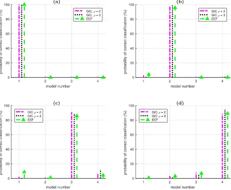
Fig. 2 shows the proportion of a correct classification for N = 25 data vectors, relative to each of the four analyzed models. The subplots refer, respectively, to the four consid-ered covariance scenarios, and the performance measures are related to three-order selectors (i.e., GIC with ρ = 2, GIC withρ=3, and EEF).
Results show that the EEF and GIC approaches provide a good performance except for the cases where symmetries lead to similar structures in the covariance matrix (i.e., azimuth and rotation symmetries), in which the probability of cor-rect classification reaches about 95%, which is more than acceptable.
B. Analysis on Real Data
Fig. 2. Probability of correct classification for N =25 data vectors. (a) Random cross-covariance matrix. (b) Reflection cross-covariance matrix form. (c) Rotation cross-covariance matrix form. (d) Azimuth cross-covariance matrix form. H1: no symmetry detected with black. H2: reflection symmetry
detected with blue. H3: rotation symmetry detected with red.H4: azimuth symmetry detected with green.
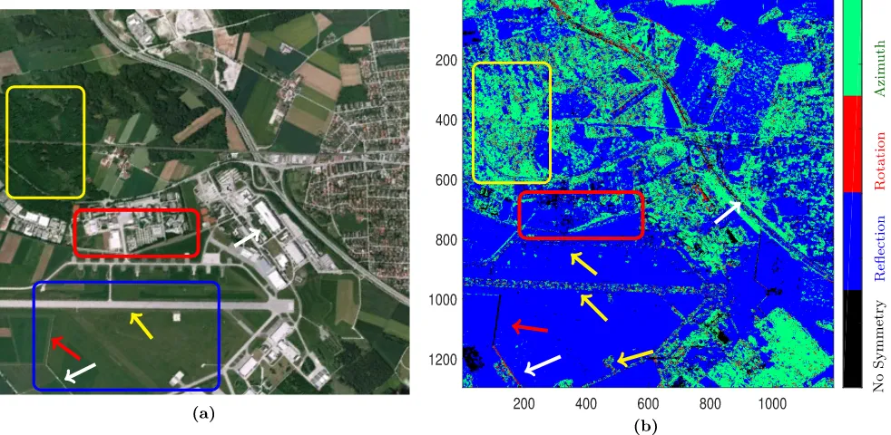
1) General Test Using GIC and EEF: As mentioned earlier, scatterers with specific geometric properties exhibit a specific symmetry. For instance, in red rectangle in Fig. 3(b), one can clearly notice the urban area manifests reflection (blue) and no symmetry (black). This is due to the fact that the urban areas contain, in general, a large amount of anisotropic scattering provided from man-made structures, which mean a nonnull degree of correlation between copolarization and cross-polarization channels [25]. This fact is manifested in the absence of both the reflection and azimuth symmetries. This is noticed clearly on the fencing of the neighboring agricultural land, indicated by the red arrow in Fig. 3(b), Notice that for the same fencing but oriented differently exhibits rotation symmetry (indicated by a white arrow).
On the other hand, the reflection symmetry implies a null correlation between copolarization and cross-polarization channels [25], which can be produced for soil surfaces without row structures [blue rectangle in Fig. 3(a)]. It is also the case for volume scattering from random layer media containing spherical particles [26] at standard frequencies (C- or L-band),
Fig. 3. (a) Optical image of the test site in Oberpfaffenhofen (Google Earth). (b) GIC index associated with the four hypotheses performed using a cross covariance matrix. H1: no symmetry with black. H2: reflection symmetry with blue.H3: rotation symmetry with red. H4: azimuth symmetry with green.
Fig. 4. GIC index associated with the four hypotheses performed using polarimetric covariance matrix. H1: no symmetry with black. H2: reflection
symmetry with blue.H3: rotation symmetry with red.H4: azimuth symmetry
with green.
azimuth symmetries in forested areas, polarimetric detection seems to confuse trees canopy with gaps between trees, which is reflected by the lack of reflection symmetry in those areas. It can also be noticed that some patterns are missed as well as lot of symmetries in comparison with the PolInSAR detection [see yellow arrows in Figs. 3(b) and 4]; for example, the aircraft runway has disappeared completely and confused with the nearby field, as well as the rotation symmetry which has greatly decreased particularly in the forested area.
Algorithm 1 H-A-αDecomposition Using Symmetry initialization ;
whilenot at end of the dataset do Data:
1) read current pixel ;
Cint= ⎛ ⎜ ⎜ ⎜ ⎝
!
ShhmShh∗ s
" √ 2
!
ShhmSh∗vs
"
ShhmSvv∗s
√
2 !
ShvmShh∗ s
" 2
!
ShvmSh∗vs
" √
2ShvmSvv∗s
!
SvvmShh∗s
" √ 2
!
SvvmSh∗vs
"
SvvmSvv∗s
⎞ ⎟ ⎟ ⎟ ⎠
;
2) Perform transformations and compute the matrices
S,S,¯ S, andS˘ ;
3) Estimate dominant symmetry using GIC/EEF of the pixel, as described in Section III ;
4) Perform the inverse transformation of the pixel matrix, and get the canonic form of the
cross-covariance matrix by eliminating noise ;
5) Extract H-A-αdecomposition starting from the new matrix form ;
end
Result: 2D H-A-α decomposition map.
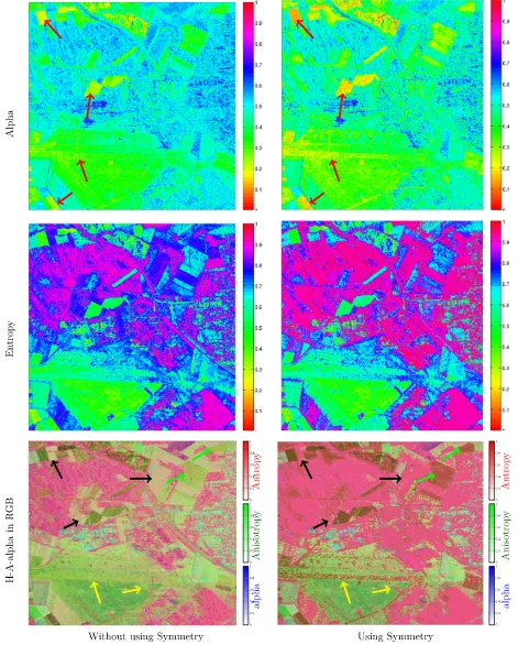
Fig. 5. Comparison between, alpha “α,” entropy “H,” and RGB of H-A-αusing symmetry properties and without (Left column contains the H-A-αperformed without using symmetries, and right column performed using symmetries).
In Fig. 5,αand H matrices are plotted with/without using the symmetries information. We have used GIC (with ρ=3, and 3×3 sliding window). From Fig. 5, we can notice that some areas appear clearer on the right side image than that of
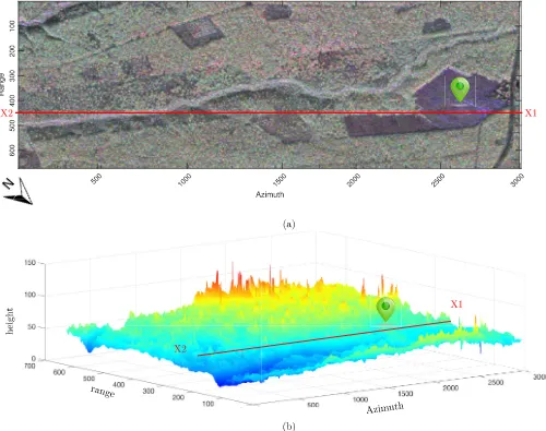
[image:9.612.71.542.62.648.2]Fig. 6. (a) Pauli-RGB coded image of the selected region (red: HH-VV, green: 2HV, and blue: HH+VV) from the BiosSAR-II data set; the region is located at 64°142.72 N latitude and 19°4752.47 E longitude (location indicated by green map marker). (b) 3-D phase difference map of the selected region of test with the surface phases contour plot on the plane. The red line indicates the row chosen as an example for phase profile with symmetries.
the scattering mechanism. If α is zero, then the mechanism is that of a canonical surface scattering. This translated the appearance of the airplane track. In the other extreme case, i.e., α = 90°, the backscattering mechanism is that of a dihedral or helices. It is known [10] that the entropy of the target is defined as the randomness indicator of the global scattering phenomenon. A zero entropy indicates that the observed target is pure and the scattering is deterministic [10], while the completely random character of the observed target is defined by an entropy equal to one. The test site consists mainly of forest or agricultural areas, and the vegetation is characterized by randomness. Consequently, most regions reach a one H ∼= 1, andthis appears more readable on the entropy made using the symmetry (right images). To give an additional evidence of the effectiveness of the approach, we have represented the H-A-αdecomposition in RGB colors, and the results do not need scrupulous attention to see the difference. For example, the aircraft track (yellow arrow in the bottom right of Fig. 5) appears as a different class compared
with the neighboring flat area in contrast to the left RGB image [Fig. 5 (bottom left)]. In addition, we notice the emergence of new areas in the forested region indicated by the red arrows [Fig. 5 (top right) and Fig. 5 (bottom) by green arrows], which are in fact a bare soil. In addition, we notice that some regions with medium-length vegetation (indicated by black arrows) are assigned to the same class as forested.
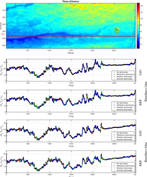
Fig. 7. (Top) Phase difference images of the test site performed using the formula (32). The four graphs correspond to the estimated horizontal phase profile associated with detected symmetries according to GIC and EEF (black: no symmetries, blue: reflection symmetries, red: rotation symmetries, and green: azimuth symmetries) carried out along the red line in Fig. 6. The two graphs on bottom correspond to an 18-m baseline, and the two other correspond to a 12-m baseline.
over a vast forested area with a variety of trees species. The BioSAR II data set is acquired at L-band over Krycklan forest site and came with a related ground truth, such as
is of 90 t/ha. The measured maximum forest height is about 30 m. The topography in the site is characterized by moderate slopes and a height variation. The objective is to use the cross-covariance matrix to detect symmetries and its related height by using DEM differencing. Fig. 6 shows the Pauli-RGB coded (i.e., red: HH−VV, green: 2HV, and blue: HH+VV) image of the selected region, where the horizontal red line denotes the phase profile transaction, which passes through homogeneous forest, groove, and an agriculture region.
For a better visual comparison, Fig. 7 shows all detected symmetries by different estimators according to GIC and EEF (black: no symmetries, blue: reflection symmetries, red: rotation symmetries, and green: azimuth symmetries), as well as their vertical positions performed using formula (32) from two different baselines, namely, 12 m (graphs on top) and 18 m (graphs on bottom) carried out along the red line. Only the PolInSAR phase difference map, scaled from 0 to 120 m, from 12-m baseline is superimposed on the top (Fig. 7). The maximum phase difference obtained with the two con-sidered baselines is 138 m for 12-m baseline and 133 m for 18-m baseline.
As shown in Fig. 7, the detected symmetries are approxi-mately the same for the two baselines more resemblance for the same detectors. Moreover, it can be observed that the difference appears mainly between the reflection and azimuth symmetries. This is caused by two main reasons: 1) the similarity between the two covariance matrices (azimuth and rotational symmetries) which disturbs the decision and 2) the difference in the angle of view between the two baselines which causes a change in the reflection geometry.
V. CONCLUSION
In this paper, we have extended a recent framework for detecting covariance symmetries to the PolInSAR data; the formulation of detecting covariance symmetries within the PolSAR data has been adapted to PolInSAR in order to detect not only the symmetry but also its associated interferometric information, by using the cross-covariance matrix instead of the cocovariance (namely, master or slave). The validation of the algorithm has been achieved using the E-SAR repeat pass PolInSAR data acquired at L-band over the Oberpfaffenhofen area in Germany. The procedure considers the GIC approach in order to deal with the multiple hypothesis testing problem (i.e., no symmetry, reflection symmetry, rotation symmetry, and azimuth symmetry), since that GIC provides good results. The fact that makes this approach more reliable is the coherent distribution of the index of symmetry, which corresponds to the theory and conforms to the ground reality, for example, the azimuth symmetry in the forested area and the reflection in surfaces.
The results were very encouraging and satisfactory and have opened a promising field of future applications, for example, it might be exploited to separate some elements over the forested areas in order to increase the accuracy of inversion methods. Moreover, it must pay attention to the promising benefits that could be drawn from PolInSAR symmetry detection, and the added value in the PolInSAR data
retrieval applications, where it can be used as a criterion to confirm the validity of the vegetation height retrieval process. For example, in the RVoG model [29], the inversion method is based on least squares line fit to find the best fit straight line inside the unit circle. And the far intersection with a unit circle to HV coherence represents the ground topography, while the height is assumed to be represented by the HV polarization. The use of symmetry, in this case, would increase the reliability of the inversion by taking it as an additional assumption, as the reflection symmetry is related mostly to the vegetation, and the azimuth symmetry can reveal about ground surfaces. Future works will be devoted to the use of this procedure for pure PolInSAR applications.
ACKNOWLEDGMENT
The authors would like to thank European Space Agency (ESA), the BioSAR Team from ESA, and the German Aerospace Center (DLR), for the data provision and for the science support.
REFERENCES
[1] S. R. Cloude and K. P. Papathanassiou, “Polarimetric SAR interferome-try,”IEEE Trans. Geosci. Remote Sens., vol. 36, no. 5, pp. 1551–1565, Sep. 1998. [Online]. Available: http://ieeexplore.ieee.org/xpls/abs_all. jsp?arnumber=718859
[2] F. Kugler, S.-K. Lee, I. Hajnsek, and K. P. Papathanassiou, “Forest height estimation by means of Pol-InSAR data inversion: The role of the vertical wavenumber,” IEEE Trans. Geosci. Remote Sens., vol. 53, no. 10, pp. 5294–5311, Oct. 2015. [Online]. Available: http://ieeexplore. ieee.org/xpls/abs_all.jsp?arnumber=7101230
[3] W. Fu, H. Guo, P. Song, B. Tian, X. Li, and Z. Sun, “Combination of PolInSAR and LiDAR techniques for forest height estimation,” IEEE Geosci. Remote Sens. Lett., vol. 14, no. 8, pp. 1218–1222, Aug. 2017. [4] M. Cariset al., “High resolution dual-channel SAR-system for airborne applications,” inProc. 18th Int. Radar Symp. (IRS), Jun. 2017, pp. 1–7. [5] S. V. Nghiem, S. H. Yueh, R. Kwok, and F. K. Li, “Symmetry properties in polarimetric remote sensing,”Radio Sci., vol. 27, no. 5, pp. 693–711, Sep./Oct. 1992. [Online]. Available: http://onlinelibrary.wiley.com/doi/ 10.1029/92RS01230/abstract
[6] D. S. Kimes, J. A. Smith, and J. K. Berry, “Extension of the optical diffraction analysis technique for estimating forest canopy geometry,”
Austral. J. Botany, vol. 27, no. 5, pp. 575–588, Oct. 1979. [Online]. Available: http://www.publish.csiro.au/bt/BT9790575
[7] M. Moghaddam, “Effect of medium symmetries in limiting the number of parameters estimated with polarimetric interferometry,” inProc. IEEE Int. Geosci. Remote Sens. Symp. (IGARSS), vol. 4, Jun./Jul. 1999, pp. 2221–2223.
[8] J. D. Ballester-Berman and J. M. Lopez-Sanchez, “Applying the Freeman–Durden decomposition concept to polarimetric SAR interfer-ometry,”IEEE Trans. Geosci. Remote Sens., vol. 48, no. 1, pp. 466–479, Jan. 2010.
[9] L. Pallotta, C. Clemente, A. De Maio, and J. J. Soraghan, “Detect-ing covariance symmetries in polarimetric SAR images,” IEEE Trans. Geosci. Remote Sens., vol. 55, no. 1, pp. 80–95, Jan. 2017.
[10] S. R. Cloude and E. Pottier, “An entropy based classification scheme for land applications of polarimetric SAR,”IEEE Trans. Geosci. Remote Sens., vol. 35, no. 1, pp. 68–78, Jan. 1997.
[11] M. Salehi, Y. Maghsoudi, and A. Mohammadzadeh, “Assessment of the potential of H/A/Alpha decomposition for polarimetric interfero-metric SAR data,” IEEE Trans. Geosci. Remote Sens., vol. 56, no. 4, pp. 2440–2451, Apr. 2018.
[12] M. Neumann, L. Ferro-Famil, and A. Reigber, “Multibaseline polarimet-ric SAR interferometry coherence optimization,”IEEE Geosci. Remote Sens. Lett., vol. 5, no. 1, pp. 93–97, Jan. 2008.
[14] F. Garestier and T. L. Toan, “Forest modeling for height inversion using single-baseline InSAR/Pol-InSAR data,” IEEE Trans. Geosci. Remote Sens., vol. 48, no. 3, pp. 1528–1539, Mar. 2010.
[15] S. R. Cloude and D. Corr, “Tree-height retrieval using single base-line polarimetric interferometry,” in Proc. ESA Workshop, PolInSAR, Jan. 2003.
[16] M. Lavalle, “Full and compact polarimetric radar interferometry for vegetation remote sensing,” Ph.D. dissertation, Inst. d’Electronique et de Télécommun. Rennes Groupe Image Télédétection, Rennes, France, Univ. Rennes 1, Dec. 2009. [Online]. Available: https://tel.archives-ouvertes.fr/tel-00480972/document
[17] J.-S. Lee and E. Pottier,Polarimetric Radar Imaging: From Basics to Applications, 1st ed. Boca Raton, FL, USA: CRC Press, Feb. 2009. [18] S. R. Cloude and K. P. Papathanassiou, “Polarimetric radar
inter-ferometry,” in Proc. SPIE, Wideband Interferometric Sens. Imag. Polarimetry, vol. 3120, pp. 224–236, 1997. [Online]. Available: https://spie.org/Publications/Proceedings/Volume/3120
[19] S. Tahraoui, M. Ouarzeddine, and B. Souissi, “Interferometric coherence optimization: A comparative study,” inProc. 8th Int. Conf. Broadband Wireless Comput., Commun. Appl. (BWCCA), Oct. 2013, pp. 427–431. [20] M. Lavalle, M. Simard, and S. Hensley, “A temporal decorrelation model for polarimetric radar interferometers,” IEEE Trans. Geosci. Remote Sens., vol. 50, no. 7, pp. 2880–2888, Jul. 2012.
[21] N. R. Goodman, “Statistical analysis based on a certain multivari-ate complex Gaussian distribution (an introduction),” Ann. Math. Statist., vol. 34, no. 1, pp. 152–177, 1963. [Online]. Available: http://projecteuclid.org/euclid.aoms/1177704250
[22] P. Stoica and Y. Selen, “Model-order selection: A review of information criterion rules,”IEEE Signal Process. Mag., vol. 21, no. 4, pp. 36–47, Jul. 2004.
[23] S. Kay, “Exponentially embedded families—New approaches to model order estimation,”IEEE Trans. Aerosp. Electron. Syst., vol. 41, no. 1, pp. 333–345, Jan. 2005. [Online]. Available: http://adsabs.harvard.edu/ abs/2005ITAES.41.333K
[24] K. Bryan and Y. Shibberu, “Penalty functions and constrained optimiza-tion,” Dept. Math., Rose-Hulman Inst. Technol., Terre Haute, IN, USA, 2005. [Online]. Available: http://www.rosehulman.edu/bryan/lottamath/ penalty.pdf and https://www.rose-hulman.edu/~bryan/lottamath/penalty. pdf
[25] J. C. Souyris, P. Imbo, R. Fjortoft, S. Mingot, and J.-S. Lee, “Com-pact polarimetry based on symmetry properties of geophysical media: Theπ/4 mode,” IEEE Trans. Geosci. Remote Sens., vol. 43, no. 3, pp. 634–646, Mar. 2005.
[26] M. Borgeaud, R. T. Shin, and J. A. Kong, “Theoretical models for polarimetric radar clutter,”J. Electromagn. Waves Appl., vol. 1, no. 1, pp. 73–89, 1987. [Online]. Available: http://www.tandfonline.com/ doi/abs/10.1163/156939387x00108
[27] J. J. van Zyl, “Calibration of polarimetric radar images using only image parameters and trihedral corner reflector responses,”IEEE Trans. Geosci. Remote Sens., vol. 28, no. 3, pp. 337–348, May 1990. [Online]. Available: http://ieeexplore.ieee.org/abstract/document/54360/
[28] K. P. Papathanassiou and S. R. Cloude, “Single-baseline polarimetric SAR interferometry,”IEEE Trans. Geosci. Remote Sens., vol. 39, no. 11, pp. 2352–2363, Nov. 2001.
[29] S. R. Cloude and K. P. Papathanassiou, “Three-stage inversion process for polarimetric SAR interferometry,”IEE Proc.-Radar, Sonar Navigat., vol. 150, no. 3, pp. 125–134, Jun. 2003.
Sofiane Tahraouireceived the Engineering Diploma (Ingenieur d’Etat) degree in electronic telecommu-nications from Saad Dahleb University, Blida, Alge-ria, in 2006, and the magistaire degree in system d’information geographique and images processing from the University of Science and Technologies Houari Boumedien (USTHB), Bab Ezzouar, Alge-ria, in 2012, where he is currently pursuing the Ph.D. degree.
He is currently a member of the Laboratoire de traitement d’image et Rayonnement, Images and Signal Processing and Radiation Research Groups, USTHB. His research interests include polarimetry, interferometry, signal/images processing applied in synthetic aperture radar, and optimization.
Carmine Clemente(S’09–M’13) received the Lau-rea (B.Sc.) and LauLau-rea Specialistica (M.Sc.) degrees
(cum laude) in telecommunications engineering from the Universita’degli Studi del Sannio, Ben-evento, Italy, in 2006 and 2009, respectively, and the Ph.D. degree from the Department of Electronic and Electrical Engineering, University of Strathclyde, Glasgow, U.K., in 2012.
He is currently a Lecturer with the Department of Electronic and Electrical Engineering, University of Strathclyde, where he is involved in advanced radar signal processing algorithm, multiple-input and multiple-output radar systems, and micro-Doppler analysis. His research interests include synthetic aperture radar (SAR) focusing and bistatic SAR focusing algorithms develop-ment, micro-Doppler signature analysis and extraction from multistatic radar platforms, micro-Doppler classification, and statistical signal processing.
Luca Pallotta (S’12–M’15) received the Laurea Specialistica degree (cum laude) in telecommuni-cation engineering from the University of Sannio, Benevento, Italy, in 2009, and the Ph.D. degree in electronic and telecommunication engineering from the University of Naples Federico II, Naples, Italy, in 2014.
His research interests include the field of statistical signal processing, with emphasis on radar signal processing and radar targets classification.
Dr. Pallotta received the Student Paper Competi-tion at the IEEE Radar Conference.
John J. Soraghan (S’83–M’84–SM’96) received the B.Eng. degree (Hons.) and the M.Sc.Eng. degree in electronic engineering from the University Col-lege Dublin, Dublin, Ireland, in 1978 and 1983, respectively, and the Ph.D. degree in electronic engineering from the University of Southampton, Southampton, U.K., in 1989, with a focus on syn-thetic aperture radar processing on the distributed array processor.
From 1978 to 1981, he was with the Electricity Supply Board, Dublin, as an Engineer, and West-inghouse Electric Corporation, Monroeville, PA, USA, as a Radar Engineer. In 1986, he joined the Department of Electronic and Electrical Engineering, University of Strathclyde, Glasgow, U.K., as a Lecturer. He was a Manager of the Scottish Transputer Center, University of Strathclyde, from 1988 to 1991, where he was the Manager with the Department of Trade and Industry Parallel Signal Processing Center from 1991 to 1995 and the Head of the ICSP from 2005 to 2007. He became a Professor in signal processing with the Department of Electronic and Electrical Engineering, University of Strathclyde, in 2003, where he held the Texas Instruments Chair in signal processing from 2004 to 2016. He is currently the Director of the Sensor Signal Processing Research Groups and the Director of the Neuromorphic Technology Laboratory within the Center for Signal and Image Processing, University of Strathclyde. His current research interests include signal processing algorithms and deep learning and neuromorphic technologies, with applications to radar, sonar, and acoustics, biomedical signal, and image processing, video and speech analytics, and condition monitoring. He has supervised 51 researchers to Ph.D. graduation and has authored over 340 technical publications. He is a member a member of the Institution of Engineering and Technology.
Mounira Ouarzeddinereceived the Degree in tronics engineering and magistaire degree in elec-tronics systems from the University of Science and Technology Houari Boumedienne (USTHB), Bab Ezzouar, Algeria, in 1993 and 1998, respectively, and the M.Sc. degree in geoinformatics and the doc-torat d’etat degree in image processing and remote sensing from the International Institute for Geo-Information Science and Earth Observation, Twente University, Enschede, The Netherlands, in 2002 and in 2008, respectively.