On the use of dynamic reliability for an accurate modelling of renewable power plants

On the use of dynamic reliability for an accurate modelling of renewable power plants

Ferdinando Chiacchio, Diego D’Urso, Fabio Famoso, Sebastian Brusca, Jose Ignacio Aizpurua, Victoria M. Catterson

PII: S0360-5442(18)30510-3

DOI: 10.1016/j.energy.2018.03.101

Reference: EGY 12559

To appear in: Energy

Received Date: 25 July 2017

Revised Date: 08 March 2018

Accepted Date: 18 March 2018

Please cite this article as: Ferdinando Chiacchio, Diego D’Urso, Fabio Famoso, Sebastian Brusca, Jose Ignacio Aizpurua, Victoria M. Catterson, On the use of dynamic reliability for an accurate modelling of renewable power plants, Energy (2018), doi: 10.1016/j.energy.2018.03.101

1 ON THE USE OF DYNAMIC RELIABILITY FOR AN ACCURATE MODELLING OF

2 RENEWABLE POWER PLANTS

3

4 Ferdinando Chiacchioa*_{, Diego D’Urso}a_{, Fabio Famoso}b_{, Sebastian Brusca}c_{, Jose Ignacio Aizpurua}d_, 5 Victoria M. Cattersond

6

7 a _{Department of Electrical, Electronical and Computer Engineering, University of Catania, Italy} 8 b _{Department of Civil Engineering and Architecture, University of Catania, Italy}

9 c _{Department of Engineering, University of Messina, Italy}

10 d _{Department of Electronic and Electrical Engineering, University of Strathclyde, Scotland} 11

12

13 ABSTRACT

14

15 Renewable energies are a key element of the modern sustainable development. They play a key 16 role in contributing to the reduction of the impact of fossil sources and to the energy supply in remote 17 areas where the electrical grid cannot be reached.

18 Due to the intermittent nature of the primary renewable resource, the feasibility assessment, the 19 performance evaluation and the lifecycle management of a renewable power plant are very complex 20 activities. In order to achieve a more accurate system modelling, improve the productivity prediction 21 and better plan the lifecycle management activities, the modelling of a renewable plant may consider 22 not only the physical process of energy transformation, but also the stochastic variability of the 23 primary resource and the degradation mechanisms that affect the aging of the plant components 24 resulting, eventually, in the failure of the system.

25 This paper presents a modelling approach which integrates both the deterministic and the 26 stochastic nature of renewable power plants using a novel methodology inspired from reliability 27 engineering: the Stochastic Hybrid Fault Tree Automaton. The main steps for the design of a 28 renewable power plant are discussed and implemented to estimate the energy production of a real 29 photovoltaic power plant by means of a Monte Carlo simulation process. The proposed approach, 30 modelling the failure behavior of the system, helps also with the evaluation of other key performance 31 indicators like the power plant and the service availability.

32

33 Keywords: Renewable Energy, Stochastic Hybrid Automaton, Availability, Photovoltaic Power Plant, Service

34 Availability

35

Nomenclature

Generic Acronyms

GHI Global horizontal irradiation

IPER Italian Producer Electrical Regulation DFT Dynamic Fault Tree

KPI Key Performance Indicator RDFT Repairable Dynamic Fault Tree

SHyFTA Stochastic Hybrid Fault Tree Automaton

Photovoltaic Power Plant

ACB Alternate current circuit breaker ACD Alternate current disconnector ACS Alternate current section

BAT Battery

DCB Differential circuit breaker DCD Direct current disconnector

DCS Direct current section GCC Grid connect coupling section GPR Grid protection

INV Inverter

PVM Photovoltaic module section PVG Photovoltaic generator PVS Photovoltaic string

SDP Surge protection (AC section) SPD Surge protection (DC section) SPR String protection

STB String box

TRA Transformer

TRK Tracker

SHyFTA Parameters

β Shape factor (Weibull function) γ Scale parameter (Weibull function)

λ Failure rate

BE Basic event HBE Hybrid basic event

Ssk_{i i}th_{stochastic state of k}th _{basic event:}

Sk1: kth basic event working (good)

Sk2: kth basic event broken (bad)

Xi ith real time variable:

XAGING_INVi Aging ith inverter

XACGi AC Power ith generator

XACS Total AC Power generated

XCONS Power consumed by utilities

XDCGi DC Power ith generator

XTA Ambient temperature

XGRID Power output to the grid

XIRR Solar irradiance

XPVSi Power ith photovoltaic string

Physical Process

α Elevation angle

β Tilt angle

η Efficiency

ηm Solar panel efficiency

ηfirst Efficiency (first year)

ηinverter Inverter efficiency

ηn Efficiency (nth year)

ηstd Efficiency (standard condition)

ρ Power coefficient

A Photovoltaic panel area Dr Degradation rate

E Energy

G Global solar irradiance Irr Incident solar irradiance

L Aging

Pk Power (kth section of power plant)

PAC Alternate current power

PDC Direct current power

Ploss Power loss

Ta Ambient temperature

Tc Solar module temperature

Tc,std Solar module temperature (standard

condition)

Stochastic Process

A Availability

Aser Service availability

SSA Steady state availability

U Unavailability

pdf Probability density function P(E) Probability ith _event

1

2 3

4 1 INTRODUCTION

5 In the last decades, the renewable energy industry has grown unceasingly and is expected to 6 increase up to 2.7 times between 2010 and 2035 [1]. Renewable energies play a key role in the 7 sustainable development of distributed generation because they contribute substantially to the 8 reduction of the impact of fossil sources, and they are the major alternative for the provision of energy 9 in remote locations where the electrical grid cannot be reached [2], or in agricultural cultivation where 10 their utilization is preferred [3, 4] to diesel generation for irrigation.

11 Renewable technologies are usually considered to be less efficient than traditional energy 12 conversion systems owing to their intermittency and energy storage difficulties. These properties limit 13 the ability of renewable power plants to fully supply peak-load and base-load [5]. For these reasons, 14 the installation of a renewable power plant can require a complex feasibility study [6] including the 15 following activities: (i) a preliminary evaluation of the installation site so as to determine the 16 availability of the primary resource, (ii) the design and the availability assessment of the power plant, 17 (iii) the estimation of productivity and the policies for the dispatch/storage and (iv) the optimization 18 strategies, including the maintenance plans. While the measurement of the primary resource 19 availability can be performed experimentally with the use of meteorological stations, satellites or 20 other types of instrumentation, the other activities for the design and management (ii)-(iv) are mainly 21 realized using engineering tools based on mathematical models.

1 fault of the system components, and allow flexible re-design and application of the model so as to 2 estimate the plant performance within a recognized tolerance. Traditional mathematical models for 3 the performance evaluation and feasibility assessment of a renewable power plant do not satisfy all 4 these properties. In fact, they do not consider the performance deterioration occurring during the 5 system lifetime and they do not account for the variability of the primary resource and its effects on 6 the power plant availability. These properties affect the quality of the system from the design stage 7 [7] and influence costs and performance predictions during the life cycle [8-10]. In renewable power 8 plants, this is even more critical because the operating conditions are continuously influenced by the 9 randomness of the renewable resource therefore the production plans and the maintenance strategies 10 must be optimized in order to increase the continuity of service [11].

11 In this context, there is room to improve the accuracy of the state-of-the-art models. This paper 12 proposes the adoption of dynamic reliability concepts [12] to overcome the limitations of traditional 13 deterministic models and achieve a more realistic description of the process of energy conversions 14 realized by renewable power plants. Dynamic reliability is a well-known modelling paradigm of 15 reliability engineering and it is mainly used to perform the evaluation of the dependability attributes 16 of an engineering system [13] that operates in non-static working conditions.

17 Dynamic reliability based approaches study the behaviour of complex systems by adopting a 18 model-based approach. This implies dealing with the thermodynamic equations to specify physical 19 processes that affect the health of system components. This methodology requires the definition of 20 the stochastic differential equations of the process and it enables forecasting performances and 21 failures while boundary conditions and independent variables can vary. The main hypothesis of 22 dynamic reliability models is that non-static working conditions affect the operation modes of the 23 system under study and its failure behaviour, e.g. the failure rates may increase or decrease under 24 certain conditions. Traditional mathematical models are not able to capture this dynamic behaviour, 25 therefore the application of dynamic reliability for the feasibility assessment and the performance 26 evaluation of a renewable power plant can provide a valuable benefit.

27 Among the possible modelling techniques of dynamic reliability, Stochastic Hybrid Fault Tree 28 Automaton (SHyFTA) [14] is well-suited for renewable power plants as it allows an extensible 29 modelling, and a simple definition of reward functions [15] for the performance evaluation and 30 feasibility assessment of a system, spreading from the dependability attributes like reliability or 31 availability to the most important design-related key performance indexes such as the service 32 availability and the productivity of a system. Moreover, a SHyFTA model can be coded and simulated 33 with a general-purpose programming language (like Python, Java, C, etc.) or implemented with a 34 high-level programming language like Matlab.

35 In this paper a structured approach to design a SHyFTA model for a renewable power plant is 36 presented. The proposed approach is discussed with the aid of a case of study of a real photovoltaic 37 power plant. The model of the power plant is built upon a previous work [16], valid only for non-38 repairable components and limited to the system reliability evaluation. This works extends [16] by 39 modelling and analyzing repairable components. Additional key performance indexes of repairable 40 systems are computed such as the power plant availability and other design-related metrics like the 41 energy production and the service availability. In order to test the accuracy of the proposed 42 methodology, the results of the SHyFTA and of the deterministic model have been compared with 43 the real data of energy production, collected by the SCADA system of the photovoltaic plant

44 The rest of this paper is organized as follows. Section 2 gives a brief overview of the state-of-45 the-art approaches. Section 3 introduces the theoretical background of the SHyFTA modelling 46 approach. Section 4 describes a real case study of a photovoltaic power plant and Section 5 shows 47 and discusses the results of the application of SHyFTA to model other renewable power plants. 48 Finally, Section 6 summarizes conclusions and discusses future work.

49

50 2 RELATED WORKS

1 the modelling of deterministic and stochastic processes independently. For instance, the design and 2 the study of renewable power plants with deterministic approaches are object of several academic 3 courses and handbooks [17, 18].

4 The analysis of the effect of the stochastic behavior of the primary resource (e.g., wind, solar, 5 hydro) onto a power plant has been recently addressed [19]. Principle component analysis has been 6 used in [20] to evaluate the wind power generation with respect to the geographic properties of the 7 installation site. In [21] it is stated that the optimization procedures of hydroelectric power plants 8 require the use of techniques able to account for the non-linear behavior of these systems, such as 9 statistical inference methods [22], evolutionary computing algorithms [23] or machine learning 10 techniques [24]. All these approaches are based on data-driven statistical learning methods and they 11 do not model the underlying physical process, i.e. they are purely statistical methods. Moreover, all 12 these works are mainly focused on the randomness of the primary resource and they overlook that the 13 performance of a system will be affected by operational conditions, components failures and, more 14 generally by the system availability that can vary continuously. In fact, availability is an important 15 characteristic of a system because it determines whether or not a system is available and if it is able 16 to perform its tasks. For this reason, this property should not be excluded when evaluating the system

17 performance.

18 The availability of a system is defined as the probability of a system to operate satisfactorily at a 19 given point in time under stated operation conditions [25]. Availability can be computed for any type 20 of industrial system comprised of different components through quantitative stochastic modelling 21 methods. In [26], Borges reviewed the most important renewable energies (wind, photovoltaic, 22 hydroelectric and biomass) proposing simplified versions of availability models made up of a small 23 set of operational states. In this work, the analysis is limited to the evaluation of the dependability 24 attributes only [25], such as reliability, availability, safety and maintainability. Moreover, it is 25 assumed a constant failure behavior and operation conditions of the system components. This last 26 assumption is common in other works [16], [27-29] in which the mean time to failure of the power 27 plant components are a fixed and independent from the rest of the system parameters.

28 There have been proposed several modelling methods which can be divided into three groups as 29 shown in Table 1, static, dynamic and hybrid-dynamic models [14, 30].

30 31

32 Table 1: Main characteristics of the models used for dependability assessment.

33

34 Static or Boolean models are the simplest models as they are based on combinatorial logic. These 35 models are not computationally demanding because the system structure function can be obtained 36 applying direct Boolean algebra that is not time-dependent [31]. Most of the reliability and risk 37 assessment reports, including many examples of renewable power plants [16], [27-29], [32-35], are 38 still based on static models.

39 Dynamic models have been introduced to handle temporal dependencies among the system 40 components. In these models, the working conditions are static but the temporal dimension affects 41 the way how the stochastic process evolves. For this reason, the resolution of dynamic models is more 42 computationally demanding than static models and is generally achieved exploiting through 43 analytical and simulation approaches [36]. The application of an analytical method depends on the 44 complexity of the model. In fact, when the system interactions can be described using only the 45 exponential distribution function, the model can be transformed into Continuous Time Markov 46 Chains and solved analytically. Unfortunately, the computational cost in terms of memory usage and 47 time of computation can increase exponentially with the number of components (i.e., state space 48 explosion). In this context simulation-based methods are used so as to model large systems with a 49 variety of probability distribution functions. Simulation-based models avoid the state-space explosion 50 at the cost of increased simulation time.

1 performance of the system. In renewable power plants this is even more critical because the operating 2 conditions (and thus the failure characteristics) are continuously influenced by the randomness of the 3 renewable resource.

4 Hybrid-dynamic models implemented through Dynamic Reliability concepts [12], have been 5 conceived to address the previous limitations and allow the modelling of non-constant failure rates 6 and dynamic operation conditions. In fact, dynamic reliability enables the link between the system 7 operation conditions and the components’ failure specification by combining the system’s physics-8 of-operation with the stochastic failure behavior of its components. These models are characterized 9 by two concurrent processes evolving and interacting in time. Therefore simulation is the most 10 suitable approach of resolution for dynamic reliability model. In these models, the computational cost 11 for the specification and analysis of two processes evolving parallel in time can be very high and time

12 consuming.

13 The main advantage of dynamic reliability is the possibility to address the evaluation of a system 14 both in terms of dependability attributes (reliability, availability and maintenance) and performance 15 (production and other relevant key performance indicators, like the service availability). Several 16 contributions in industrial [37] and nuclear applications have already shown the improved accuracy 17 of this modelling paradigm [14, 38], supported also by other works [39-43] addressing the evaluation 18 of the failure rates with respect to the system working conditions. Unfortunately, the failure behavior 19 of a system component with respect to the system operating conditions is not always known [44, 45] 20 and this represents the most important limitation for the use of dynamic reliability approaches. 21 To the best of authors’ knowledge, dynamic reliability has not been used to model renewable 22 power plant systems. With the application of the SHyFTA, this paper covers this gap and shows the 23 potentiality of dynamic reliability applications.

24

25 3 HYBRID-PAIR MODELLING OF RENEWABLE POWER PLANTS: CONCEPT AND

26 IMPLEMENTATION OF A STOCHASTIC HYBRID FAULT TREE AUTOMATON

27 This section presents the theoretical concepts of hybrid-pair modelling [46] and Stochastic 28 Hybrid Fault Tree Automaton (SHyFTA) [14], with the aim to provide the knowledge-base for 29 designing a dynamic reliability model of a renewable power plant.

30 Dynamic reliability defines a mathematical framework which is able to combine deterministic 31 (e.g., process of energy transformation) and stochastic (e.g., process of failure of a system) models 32 [12]. Dynamic reliability makes use of non-linear functions to adapt the system failure probability 33 according to the system operation conditions. This leads to more accurate reliability modelling able 34 to account for environmental and operational changes of the working conditions. Moreover, recent 35 works have shown its potential as a tool for the dimensioning of a system [46] and the understanding 36 of other aspects of the life cycle of a system that characterizes the regime operations, like availability

37 and maintenance.

38 The hybrid-pair approach was conceived to simplify the modelling effort of complex systems 39 and solve dynamic reliability problems. The main assumption of this paradigm is to break the system 40 down into two interdependent processes (deterministic and stochastic), which can interact by means 41 of shared variables. In this way, a change of the deterministic model triggers the stochastic model and 42 vice versa. One of the strengths of the hybrid-pair modelling approach is the ability to combine a 43 dependability assessment of a system with its performance evaluation.

44 When implementing the hybrid-pair model for renewable power plants, the process of energy 45 transformation operated by the power plant must be broken into two parts as shown in Figure 1: the 46 deterministic block defines the physical equations of the energy transformation whereas the stochastic 47 block models the system failure logic.

1 described with a repairable dynamic fault tree (RDFT) [49] for an easy implementation and evaluation 2 of the failure model of the system [50].

3 In the evaluation of renewable power plants, the SHyFTA can improve the accuracy with respect 4 to traditional deterministic approaches because it integrates a stochastic model of the system that 5 accounts for the dynamic evolution of the system, its variables (including the randomness of the 6 primary resource) and the fault and performance degradation states. The benefits of this technique 7 are twofold: system health state tracking and a more realistic estimation of the power plant activities. 8 In the next sections, the SHyFTA formalism is recalled and the steps for the design of a renewable 9 power plant system are pointed out.

10

11 Figure 1: Mutual dependency between the deterministic and the stochastic model.

12

13 3.1 Stochastic hybrid fault tree automaton (SHyFTA)

14 The formal mathematical formulation of SHyFTA is presented in [14]. In this subsection minimal 15 necessary concepts will be introduced. Interested readers can refer to [14] for more details.

16 The SHyFTA is a 13-uplet (𝑆, Ɛ, X, 𝛶,δ, 𝐻,𝐺, 𝐹, 𝑃, 𝐺𝐴, 𝐵𝐸,𝑇, 𝐶), where:

17  𝑆 is a finite set of discrete states {𝑆D, 𝑆S}. 𝑆Dis the subset of deterministic states and 𝑆S is the 18 subset of stochastic states.

19  Ɛ is a finite set of events {ƐD, ƐS}, where ƐDis the subset of deterministic events and ƐSis the

20 subset of stochastic events.

21  Χ is a finite set of real variables evolving in time {x1, …, xn}.

22  Υ is a finite set of arcs of the form ( , 𝑠 ɛj, Gk, ’) where and ’ are, respectively, the origin and 𝑠 𝑠 𝑠 23 the destination states of the arc k, ɛj is the event associated with this arc, Gk is the guard condition 24 on the real variable in state .X 𝑠

25  δ: 𝑆× X→(ℝ𝑛+→ℝ) is a function of activities, describing the evolution of real variables in each

26 discrete state.

27  𝛨 is a finite set of clocks on that identify the firing of a deterministic or a stochastic event.ℝ 28  F: 𝛨× 𝑆× X→(ℝ𝑛+→[0, 1]) is a set of applications that associate a distribution function to the 29 stochastic events , according to the clock H, the system evolution and the discrete state .ƐS Χ 𝑆 30  P is the instantaneous probability to be in 𝑠i ∈𝑆S;

31  GA is the finite set of gates of the fault tree model.

32  BE is the finite set of basic events of the fault tree model. The set BE contains a subset called 33 Hybrid Basic Events (HBE) whose failure distribution depends on the evolution of the system 34 and varies continuously in time. This type of basic event accounts for the multi-state nature of a 35 component, namely those systems whose failure characteristics are not static in time but vary 36 dynamically according to the operational conditions that, in turn, affect reliability and 37 performance. These events are characterized by a non-static pdf through a set of functions𝑓_𝑖∈ 𝐹, 38 𝑓_𝑖:𝛨× 𝑆× X→

(

)

39  TE is the top event of the fault tree and corresponds with the output of the main gate. 40  C is the set of connections between gates and basic events.

41 To design a fault tree model the designer needs to identify a top-event T, representing an undesired 42 operational condition of the system and its elementary causes. These causes are combined through 43 temporal and logic gates (AND, OR, VOTING k/N, PAND, SPARE, FDEP, SEQ) [49] to define the 44 occurrence of the top-event.

1 λ(t) = β/γ∙(t/γ)β ‒1 (Eq. 1)

2 Moreover, the non-linear relationship with the mission time can be described by a piecewise 3 deterministic Markov process, using the following ordinary differential equation:

4 dL_dt = i_on i_on=

{

5 Integrating Eq. (2) and substituting L(t) into Eq. (1) it is possible to rewrite the Weibull distribution 6 with the non-linear aging L(t):

7

8 λ(L) = β/γ∙(L/γ)β ‒1 (Eq. 3)

9

10 The Weibull probability density function in Eq. (3) can be generalized when the scaling factor γ 11 (L,X,S) is a function of the evolution X={x1, …,xn}and state S={𝑆 𝑆D, S}of the system. In other words, 12 the scaling factor changes with respect to the status and working conditions of the component. 13 Current hesitancy in the use of dynamic reliability models is mainly caused by the unavailability 14 of exact models of γ(L,X,S) which account for all the possible variations of the working conditions 15 [44, 45]. Recently, with the advance of condition-based monitoring techniques, reliability estimations 16 are being improved with up-to-date degradation and operation information [39-43]. In the definition 17 of a fault tree, the SHyFTA model supports both traditional and hybrid basic events. Therefore the 18 application of a variable probability failure distribution function can be limited only to those 19 components for which this information is available. In all the other cases, it is still suggested to use 20 the failure rate provided by the component manufacturer.

21 3.2 Design of a SHyFTA model for a renewable power plant

22 The main steps for the design of a SHyFTA model are shown in Figure 2. The first activity consists 23 in the study of the power plant and the identification of the discrete components that, with their 24 interaction, realize the process of energy conversion. The complexity of the deterministic process can 25 vary and depends on the amount of detail and interactions modelled. The mathematical equations 26 should describe the contribution of each component at different working regimes. Generally, this 27 representation assumes the form of a balance equation expressed in terms of a set of algebraic, 28 ordinary or partial differential equations.

29

30 Figure 2: Steps for the construction of a SHyFTA model.

31

32 The main input of the deterministic process is the time-series of the primary renewable resource 33 and of the variables that can affect the process of energy transformation. Table 2 displays the main 34 physical inputs for different renewable technologies.

35

36 Table 2: Main physical inputs for different renewable technologies

37

1 the basic event is referred as hybrid. Otherwise, the basic event must be characterized with the pdf 2 provided by the component manufacturer that is generally static.

3 The formulation of the SHyFTA is completed when the stochastic and the deterministic models 4 are coupled through shared variables. Namely, the physical variables that affect the operating 5 conditions of a component (modifying the pdf of a hybrid basic event) are synchronized in the fault 6 tree model. On the other hand, the events occurring in the stochastic model, like the failure of a 7 component are transferred to the deterministic model. In this way the contribution of the failed 8 component is nullified in the physical process of the deterministic model (e.g., an inverter that fails 9 will no longer output AC power).

10 Although the complete shutdown of a renewable power plant constituted by several generating 11 units is very unlikely, the modelling of this scenario as the Top Event of the fault tree allows the 12 evaluation of several performance indicators. Among them, the instantaneous active and reactive 13 power, the energy production within a time-period and the service availability, Aser that corresponds 14 with the probability of the renewable power plant to produce a base power and guarantee the 15 continuity of service [11, 54] for a well-defined demand curve. These key performance indicators 16 (KPI) can provide important indications for suitable dimensioning of the power plant and the life 17 cycle activities like production plans and the maintenance schedule.

18

19 4 CASE STUDY: A PHOTOVOLTAIC POWER PLANT

20 There have been proposed different fault tree models of renewable power plants that can be used 21 as reference models to build up a SHyFTA [16, 32-35]. In this paper, the case study of a photovoltaic 22 power plant is presented. The analyzed power plant is a grid-connected photovoltaic power plant with 23 no trackers implemented by a private company in 2011, located in Sicily close to Syracuse (see Figure 24 3 and Table 3).

25

26 Table 3: PV system characteristics.

27 28

29 The power plant is characterized by a peak power, Ppeak = 419,5 kW and by two identical DC/AC 30 inverters of 220 kWp. There are 4 string boxes for each inverter: 3 accommodate 17 strings and 1 31 accommodates 18 strings. The strings are connected in parallel while the modules are in series 32 (Figures 4 and 5). Tables 4-5 summarize the main characteristics of the system.

33

34 Table 4: PV module main characteristics.

35

36 Table 5: Inverter main characteristics.

37 38 39

40 To be compliant with the Italian Producer Electrical Regulation (IPER) of 2011 (Terzo Conto 41 Energia [55]), the power plant is connected to the national grid. The IPER states that the power plant 42 must stop in case of disconnection from the national grid and forbids the use of energy storage 43 systems. There is a strong economic advantage for adhering to the IPER of 2011. In fact, for the first 44 20 years of life of the power plant, there is a fixed economic subsidy for all the energy produced. 45 Moreover, the energy not instantaneously consumed by the producer is tracked and sold with a price 46 dictated by the energy market. Therefore, the power plant contributes to the company activities by 47 supplying the internal consumption and providing a profit due to the economic incentive (subsidy) 48 and the sale of the energy not consumed. Table 6 shows the value of the Subsidy (it is fixed by the 49 IPER [53]) and the corresponding price of buy/sell per one kWh of energy. This latter is a rough value 50 of the energy price in the energy market (2011). The column Total is the sum of the previous 51 contributes and it is used to estimate the payback generated by the energy produced by the power

52 plant.

1 Table 6: IPER 2011 Subsidy. Price* is based on an average value of the energy price in the energy market

2 (2011) [43].

3

4 Figure 4 shows the Global Horizontal Irradiation (GHI) in Italy. It suggests the average annual 5 productivity expressed in kWh that one meter square of photovoltaic panels can generate. It is 6 possible to notice that in the area of Syracuse, the GHI is higher than in the rest of the country. In 7 this context, the application of a model that includes possible downtimes and performance 8 degradation can help to better estimate the payback generated throughout the life time of the power

9 plant.

10

11 Figure 4: Global horizontal irradiation in Italy.

12

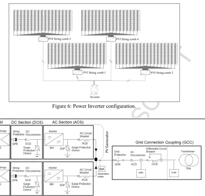
13 With reference to Figures5, 6 and 7, it is possible to identify the main components of the 14 photovoltaic power plant.

15

16 Figure 5: Map of the power plant and its sections.

17

18 Figure 6: Power Inverter configuration.

19

20 The components of the photovoltaic power plant can be grouped into the following functional 21 blocks (Figure 7):

22

23 1) PV Module (PVM),constitutes the PV module strings of the power plants (PVS);

24 2) Direct Current Section (DCS), made up of string protection diodes (SPR), DC disconnectors

25 (DCD) and surge protection devices (SPD);

26 3) Alternating Current Section (ACS),made up of inverters (INV), surge protection devices

27 (SDP) and AC circuit breakers (ACB);

28 4) Grid Connector Coupling (GCC), made up of grid protection (GPR), an AC disconnector 29 (ACD), a differential circuit breaker (DCB) and a transformer (TRA).

30

31 Figure 7: Schematic decomposition of the PV system

32

33 Next, we apply the steps discussed in Section 2 to build up the SHyFTA model under the following

34 assumptions:

35 1- The physical variables, input of the model, are the ambient temperature and sun irradiance; 36 2- The hourly aggregated samples of the physical variables are extracted by the SCADA of the

37 PV power plant;

38 3- The randomness of the physical variables is achieved by applying a random seasonal variation

39 component at each iteration of the simulation;

40 4- It is assumed that the inverter switches on when the output power at the PVM stage is greater 41 than zero (during the daily time). This affects the aging of the inverter.

42 5- In the deterministic model, performance degradations occur only for the photovoltaic panels

43 and for the inverters.

44 6- In the stochastic model, the components of the photovoltaic power plant can be only in two 45 possible states (S1: good or working, S2: bad or failed).

46 7- Failure rates of all the components except inverters are constant [16];

47 8- The inverter failure rate is not constant and is subjected only to an aging process; 48 9- Repair rates of all the components are constant;

49 10- Restoration of a component brings the component back to as-good-as-new state.

50

51 4.1 Definition of the Deterministic Process

1 series and parallel to constitute a panel. In the same manner, several panels are connected to form 2 arrays of generators and sum up to a higher direct current (DC) power.

3 As a first approximation, the electrical power generated with a simple configuration of a 4 photovoltaic string of panels can be defined as follows:

5

6

P =

ηIrr

sin (

α

+

β

)A

7

8 As shown in Figure, Irr is the incident solar irradiance [W/m2_{]; α is the elevation angle and β is the} 9 tilt angle of the module/string measured from the horizontal. Finally,A is the area of the module [m2_] 10 and ƞ is the system efficiency that is always less than 1.

11

12 Figure 8: Solar Irradiation, elevation angle α and tilt angle β 13

14 The total efficiency can be expressed as: 15

16

η

=

∏

i = 0

η

17

18 where ηis the number of loss effects considered at each ith _{stage of the power plant.}

19 At the PVM stage, meteorological factors (e.g., wind speed, cloud transients in PV units, incident 20 irradiance or ambient temperature) or yearly deterioration can reduce the efficiency of the 21 photovoltaic modules. Using Eq. (6) we can compute the efficiency of the module, ƞm

,

23

24

{

η

=

η

{1

‒ ρ(

T

‒

T

)}

G

= constant

25 Where ƞstd and Tc,std are respectively the efficiency and the module temperature at standard conditions, 26 ρ is the power coefficient (percentage variation of power for 1°C ), Tc and Ta are the module and 27 ambient temperatures and G is the global irradiance on the module.

28 To account for the degradation rate, Dr, corresponding with the percentage of efficiency lost 29 every year [57, 58], it is possible to use a linear equation model [56]:

30

31

η

=

η

(1

‒

n × D

)

33 where ƞfirst is the nominal efficiency at the first year, while ƞn is the efficiency calculated at the nth

34 year.

35 The performance degradation occurring in the PVM stage reduces the DC power, but does not 36 stop the power production unless the DC breakers and disconnectors of the DCS stage interrupt the 37 circuit or the cables fail. In fact, with reference to Figure 7, a single PV generator can contribute to 38 the power generation of the system if the circuit path from the PVM stage to the GCC is closed. 39 Before connecting to the grid, the DC current is converted into alternating current. The DC/AC 40 inverter of the AC section performs this transformation with an efficiency that depends on the input 41 load. At this stage, inverters can also affect the performance of the system and the algebraic model 42 presented in [59] illustrates this effect:

43

44

η

=

DC

= 1

‒

P_loss

P(t)_DC

45

1 𝑃_𝐴𝐶𝑆(𝑡)= 𝑃_{𝐴𝐶𝑆1}(𝑡)+𝑃_{𝐴𝐶𝑆2}(𝑡) (Eq. 9) 2

3 For this reason, it is possible to understand that the photovoltaic plant is able to produce energy 4 if at least one of the two PV generators is in operation. To compute the energy produced and measured 5 by the generation meter (GM) before the GCC stage it is possible to integrate the PPROD in the time 6 interval [t2, t1]:

7

8 𝐸_{𝑃𝑅𝑂𝐷}(𝑡)=∫𝑡2 (Eq. 10)

𝑡1𝑃𝐴𝐶𝑆(𝑡)𝑑𝑡

9

10 The power transferred to the grid is the power not instantaneously consumed by the utilities 11 connected to the power plant. Therefore it is possible to write the equation:

12

13 𝑃_{𝐺𝑅𝐼𝐷}(𝑡) = 𝑃_𝐴𝐶𝑆(𝑡)‒ 𝑃_{𝐶𝑂𝑁𝑆}(𝑡) (Eq. 11)

14

15 When PGRID is negative, it means that the power plant is not able to satisfy the demand of power for 16 the utilities connected, resulting in a lack of service availability.

17 The other components involved in a photovoltaic system are protection, cables, breakers, 18 disconnectors and transformers. All these components play an important role in the energy production 19 because if one of them interrupts the circuit path to the GCC, the PV generator in the open path cannot 20 contribute to the power generation. This is a very critical aspect of the production process, in 21 particular when considering the elements of the GCC stage. In fact, if one of the components of the 22 GCC stage interrupts the circuit path, all the power plant stops the production because it gets 23 disconnected from the national grid, causing the complete system unavailability. To determine the 24 impact of these circumstances to all the production process the stochastic fault tree model has to be 25 designed and linked to the deterministic model.

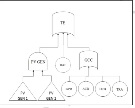
26 4.1 Definition of the Stochastic Process

27 The fault tree model in Figure 9 describes the failure behavior of the plant. This model is 28 constituted by an OR gate (TE) that takes as input an OR gate (GCC = OR (GPR, ACD, DCB, TRA)) 29 and an AND gate (PV GEN = AND (PV GEN 1, PV GEN 2)), modelling the failure behavior of the 30 PV generators. The plant production unavailability occurs if both PV generators fail or if one of the 31 components of the GCC fails.

32 Figure 10 shows the failure behavior of a single PV generator.The failure/repair rates of the 33 components are shown in Table 7. Failure rates have been taken from [1]. Note that only the inverter 34 has been modeled as a hybrid basic event whose Weibull probability distribution of failure depends 35 on the aging variable. This latter is bounded to the solar radiation input because the inverter switches 36 on when the solar irradiation is high enough to put the PV strings in operation, with a DC voltage 37 greater than the switch on threshold of the inverter. Otherwise, the inverter stays in stand-by mode, 38 waiting for the sun irradiance to increase (e.g. during the night time).

39 As for repair rates, it was assumed that electrical components like breakers, disconnectors, string 40 box and protection can be restored to as-good-as-new within two working days after a fault.

41 According to the agreements with the inverter manufacturer, the repair of the inverter takes between 42 three and four weeks, considering the whole process of inspection, ordering, delivery and 43 replacement. For PV strings it was assumed a periodic inspection would take place every six months. 44

45 Table 7: Failure/repair rates and steady state availability of the components of the PV plant.

46

47 Figure 9: Fault tree of the PV power plant. PV GEN 1 and PV GEN 2 are represented with the transfer gate

48 symbol (triangle) because these sub-systems are developed into another fault tree model.

49

50 Figure 10: Fault tree of a PV generator. The basic event INV is represented with a dashed circle to indicate

1

2 5 COUPLING AND SIMULATION OF THE SHYFTA MODEL

3 Figure 11 depicts the hybrid-pair model of the case study with the corresponding mapping into a 4 SHyFTA where it is possible to identify the main discrete components of the PV system, the 5 corresponding real time variables Xi of the deterministic process and the vector ƐS encoding the status 6 of the basic events of the stochastic process.

7

8 Figure 11: Hybrid-Pair architecture of the case study and corresponding SHyFTA mapping.

9

10 XIRR and XTA represent respectively the sun irradiance Irr and the ambient temperature Ta. These 11 two variables are inputs of the model and, according to Eqs. (4-7), affect the power generation and 12 the conversion efficiency of the PVM components. The ACS conversion depends on Eq. (8) and the 13 actual energy produced by the power plant is described by Eqs. (9) and (10). To account for the effects 14 of the stochastic model, the SHyFTA provides a mechanism of synchronization between the variables 15 of the deterministic model and the stochastic events (the basic events) that determine the status of 16 each component. In the stochastic process, the basic events are characterized by two operational 17 states, 𝑆S= {Good, Bad}. The health status of each basic event is an element of the vector ƐS that, as 18 input to the deterministic process, realizes the coupling between the basic events of the stochastic 19 process with the corresponding discrete components modelled in the deterministic process. Since it 20 was assumed that components can be only in two possible states, the binary representation can be set 21 as follows:

22

23 S_BEi=

{

th

component is working 0, ith component is failed

24

25 According to this notation, it is now possible to evaluate and rewrite the real variables 26 XPVS1/138,XDCG1/2, XACS1/2, XPROD and XGCC of the SHyFTA model that correspond with the powers 27 levels generated at the different stages of a PV plant generator.

28 XPVSi , with i=1,…,138, is the DC power generated by the ith photovoltaic string (each string is 29 comprised of 16 modules, see Table 4) that depends on the status of the ith _{string S}

PVSi: 30

31 X_PVSi=

[

(

)

]

33 XDCS1/2 are the total DC power of each photovoltaic generator (a DC generator is comprised of 34 69 strings of the corresponding PVM section)and it includes the loss of DC wiring connections and 35 possible faults of DC protection or fuses:

36

37 X_DCS1=∑69 ) (Eq. 13)

i = 1XPVSi× (SSPR1× SDCD1× SSPD1

38

39 X_DCS2=∑138 ) (Eq. 14)

i = 70XPVSi× (SSPR2× SDCD2× SSPD2

40

41 XACS1/2 are the total AC power output of each AC sections and including the efficiency loss of 42 the inverters and possible faults of the AC protections and breakers.

43

44 X_ACS1=

η

1 It is possible to notice that the components of the stage GCC can break the circuit path towards 2 the grid. When this happens, the inverter stops the DC/AC conversion and the production of the power 3 plant is nullified. In this case, during this outage, XACS1(t) =XACS2(t) = 0.

4 XACS is the total AC power generated by the photovoltaic power plant. It is measured at the 5 exchange meter of production in order to quantify the amount of energy produced that is rewarded 6 with the subsidy tariff of the IPER 2013:

7

8 X_ACS= X_ACS1+ X_ACS2 (Eq. 17)

9

10 XGRID is the power exchanged with the grid and is computed as difference between the produced 11 power XACS and the amount of instantaneous power XCONS requested by the utilities connected to the

12 power plant:

13

14 X_GRID= X_ACS‒ X_CONS (Eq. 18)

15

16 Among the variables computed in the deterministic process, Eq. 19 models the counter of the 17 inverter aging of an inverter, Xaging = L, measuring the amount of time in which an inverter is on. 18

19 X_{Aging_INVi}=∫t , i =1, 2 (Eq. 19)

0i_{ON_INV}

i

(t)dt

20

21 i_{ON_INVi}(t) =

{

DCSi= 0

22

23 This value is an input of the Weibull pdf characterizing the failure behavior of the inverter in the 24 stochastic process [see Eq. (2-3)].

25 The SHyFTA model has been coded in Matlab® to implement a software resolution based on a 26 discrete event Monte Carlo simulation [60]. Several trials must be performed in order to achieve the 27 desired accuracy (or confidence interval) of the measure to compute. For the photovoltaic power 28 plant, the focus is on the power production measured at the generation meter, XACS. Therefore, at 29 each trial k of the Monte Carlo simulation, the output of the SHyFTA model is the time-series

30 Xk

ACS(t). When the desired confidence interval is met the simulation is stopped and the mean active 31 power for each sample of the time series is computed as follows:

32 𝔼

[

(

)

]

[

𝑘= 1𝑋

𝑘

ACS(𝑡)

]

33 where N is the number of Monte Carlo trials.

34 The estimator error associated to the desired confidence interval can be computed as follows

35 [61]:

36 𝐸𝑟𝑟=𝑍_𝑎2× 𝜎_𝑁 (Eq. 21)

37

38 where Za/2 is the confidence coefficient, a is the confidence level, σ is the standard deviation of the 39 Monte Carlo simulation and N is the number of Monte Carlo trials.

40 The use of the active power as an estimator of the Monte Carlo simulation has an advantage. In 41 fact, it can be noted that the cumulative error, made up by the instantaneous samples of the time series 42 XACS(t), corresponds to an energy. In this way, it is possible to provide an appropriate estimation of 43 the active energy aside a confidence interval using the cumulative error of the estimator.

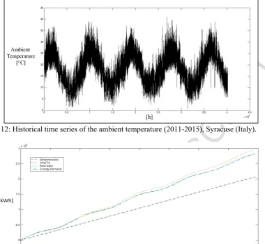
1

2 Figure 12: Historical time series of the ambient temperature (2011-2015), Syracuse (Italy).

3 5.1 Energy production estimation

4 In order to test the accuracy of the proposed methodology, the results of the SHyFTA and the 5 deterministic models have been compared with real energy production data, collected by the SCADA 6 system of the photovoltaic plant. The collected data includes the hourly aggregated power, energy, 7 solar irradiance and external temperature for the first four years and half of life, corresponding to

8 40.173 hours.

9 For the SHyFTA simulation, a confidence level of 0,99 was set for each data point XACS(t). There 10 was not set a stopping condition for the simulation and with 10.000 iterations, the cumulative absolute 11 error of the time series sums up to the 0,16%, that corresponds to ±4.681 kWh.

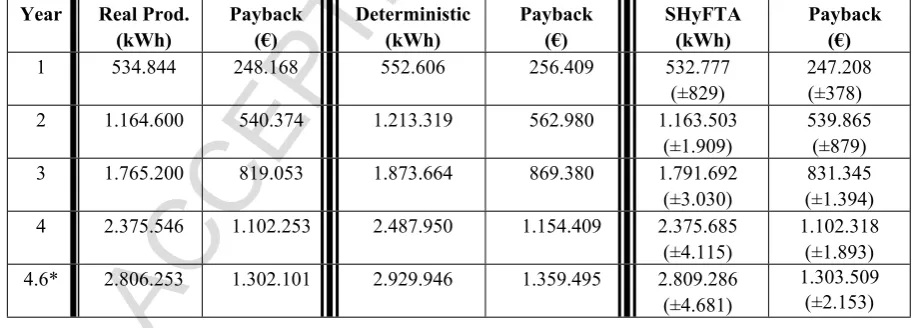
12 To compute the energy production from the time-series of the estimated active power XACS(t)Eq. 13 (20) must be used. Table 9 displays a comparison among the real data, the deterministic and the 14 SHyFTA models in terms of energy produced and payback generated under the regime of IPER 2011. 15 It is possible to notice that the results of the SHyFTA at the end of the observation period (see last 16 row of Table 8) matches with the real data aside the absolute error of the Monte Carlo simulation 17 (±4.681 kWh). It can be observed that at the beginning of the simulation, the deterministic and the 18 SHyFTA model are very close to the real data and the reason is that at the beginning of the power 19 plant life there are no faults and performance degradation which affect the system. However, after a 20 few months, the gap between the real data and the deterministic model starts to increase, whereas the 21 difference with respect to the SHyFTA remains bounded to a maximum relative error of 2%, as shown 22 in Figure 14 that plot the absolute relative error with respect to real data.

23

24 Table 8: Comparison among the real data, the deterministic and the SHyFTA model in terms of energy

25 produced and positive payback generated under the regime of IPER 2011.

26 27

28 Figure 13: Comparison between the energy produced by the deterministic model, the SHyFTA and the real

29 system.

30

31 Figure 14: Comparison between the relative error of the deterministic model and the SHyFTA.

32

33 At this point, having tested the accuracy of the proposed method, it is possible to forecast the 34 production of energy over 20 years of life in order to provide the owner of the plant with a more 35 accurate estimation of production and economical revenues. To achieve this result, the simulation 36 with the SHyFTA is extended to 20 years assuming that the physical input of the solar radiation and 37 ambient temperature follow the same evolution described by the historical time series of the last 5 38 years. The Monte Carlo simulation has been set such to respect the same confidence level of the 39 previous simulation. Under this setting, the absolute cumulative error of the time series sums up to 40 0,18%, that corresponds to ±20.480kWh.

41 Figure 15 shows the results obtained and Table 9 allows a further comparison between the 42 deterministic and the SHyFTA. In this case, it is possible to recognize at the end of the 20th _{year, a} 43 difference of about 545.000 kWh (±20.480 kWh)of loss of energy productivity. Under the regime of 44 IPER 2011, at the end of the economic investment established at the 20th _{year from the start of the} 45 power plant, this lack of energy production corresponds to a cash short of about 250.000 € (±9.421

46 €).

47

48 Figure 15: Energy production estimation throughout the life time of the power plant (20 years).

1 Table 9: Comparison between the deterministic and the SHyFTA model throughout the remaining years of the

2 plant life in terms of energy produced and positive payback generated under the regime of IPER 2011.

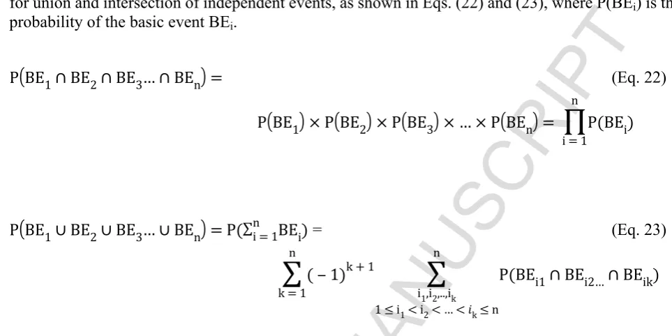
3 5.2 Plant and service availability

4 To compute the plant availability, it is possible to use the main principles of the probability theory 5 for union and intersection of independent events, as shown in Eqs. (22) and (23), where P(BEi) is the 6 probability of the basic event BEi.

7 8

9 P

(

)

10 P

(

)

(

)

(

)

(

)

n

∏

i = 1

P(BE_i)

11 12 13

14 P

(

)

i = 1BEi)

15

n

∑

k = 1

(‒1)k + 1

n

∑

i₁,i₂,..,i_k 1≤i₁< i₂< … <𝑖_k≤n

P(BE_i1∩BE_i2…∩BE_ik)

16

17 In the following relationships, P(Ei) corresponds with the unavailability Ux of each component 18 that can be obtained as Ux=1-SSAx. Table 10 reports the steady state availability for each component 19 of the Fault Tree, with the exception of the inverter that cannot be computed with the same formula, 20 valid for the exponential distributions, 𝜇/(𝜆+𝜇).

21 The failure behavior of the inverter has been modelled with a piecewise deterministic Markov 22 Process and it has a non-linear relationship with the aging of the inverter.To compute the inverter 23 availability, a dedicated simulation was performed assuming to extend the mission time and the solar 24 radiation to 20 years, by replicating the time-series of the solar radiation and ambient temperature.

25 Figure 16 shows that the steady state availability (SSA) oscillates around the values 0,98±0,001. 26

27 Figure 16: Inverter Availability simulated.

28

29 Substituting the values of the steady-state availabilities in Table 9, it is now possible to compute 30 the unavailability of each gate and, from bottom up, retrieve the system availability.

31

32 A = 1‒U_TE = 0,9999 33

34 U_TE= U_PVGEN+ U_GCC–[U_PVGEN× U_GCC] = 1e-5 35

36 U_GCC= U_GPR+ U_ACD+ U_DCB+ U_TRA–[U_GPR× U_ACD]–[U_GPR× U_DCB]–[U_GPR× U_TRA]‒[U_ACD×

37 U_DCB]‒[U_ACD× U_TRA]‒[U_DCB× U_TRA] + [U_GPR× U_ACD× U_DCB] + [U_GPR× U_ACD× U_TRA] + [

38 U_GPR× U_DCB× U_TRA] + [U_ACD× U_DCB× U_TRA]‒[U_GPR× U_ACD× U_DCB× U_TRA] =

39 0.1e-4.

40

1 For each ith _{section of the photovoltaic power plant, with i = 1, 2, it is possible to compute the}

2 following:

3

4 U_PVGENi = U_ACSi+ U_DCSi–[U_ACSi× U_DCSi] =7,5e-5 5

6 U_ACSi = U_INVi+ U_SDPi+ U_ACBi–[U_INVi× U_SDPi]–[U_INVi× U_ACBi ] –[U_SDPi× U_ACBi] + [U_INVi×

7 U_SDPi× U_ACBi] = 4,5e-5

8

9 U_DCSi = U_SPRi+ U_DCDi+ U_SPDi+ U_PVMi –[U_SPRi× U_DCDi] –[U_SPRi× U_SPDi]–[U_SPRi× U_PVMi]‒[

10 U_DCDi× U_SPDi] – [U_DCDi× U_PVMi]‒[U_SPDi× U_PVMi] + [U_SPRi× U_DCDi× U_SPDi] + [

11 U_SPRi× U_DCDi× U_PVMi] + [U_SPRi× U_SPDi× U_PVMi] + [U_DCDi× U_SPDi× U_PVMi]‒[

12 U_SPRi× U_DCDi× U_SPDi× U_PVMi] = 3e-5

13

14 U_PVMi= ∏ = 1e-13, with

jU_PVSj j =

{

1,j = 1,…, 69 2, j = 70,…, 138

15

16 According to these results, is possible to conclude that the SSA of the power plant is very high. 17 An important difference with respect to the work in [16] is that in the presented model the components 18 can be repaired after a fault. Moreover, the power plant is composed of two redundant generating 19 sections (PVGen1 and PVGen2) and both must fail before the system fails. This configuration results 20 in an increased system availability.

21 For this type of system, a more valuable KPI than reliability or availability of the system is the 22 service availability [54] that measures the probability of the system to satisfy the instantaneous power 23 demand of the connected load. In fact, reliability does not consider restoration and, in these types of 24 applications, this is not realistic. On the other hand, the classic definition of availability, intended as 25 the probability that at the observed time the system will be in production, is not very significant 26 because, as already explained, the complete shut-down of the power plant is very unlikely, as it is 27 constituted by several independent groups of generators with a high availability.

28 Service availability can be computed as the ratio between the total time in which the photovoltaic 29 power plant is not able to meet the power demand of the company and the total duration of the mission 30 time. To evaluate this KPI, three types of power unavailability must be considered:

31 i. Unavailability of generated power due to conventional outages of plant and apparatus;

32 ii. Unavailability of generated power due to source variability (power plant equipment remaining

33 perfectly healthy and operational);

34 iii. Unavailability of generated power due to outages of plant that arise due to source variability 35 (such as PV panel outages due to differential overheating that arise out of cloud transients). 36

1 2

3 Figure 17.a: daily power demand. Figure 17.b: schema of the power supply.

4

5 The results of the SHyFTA match exactly the real scenario (Table 10). It is possible to notice that 6 the service availability is much lower than the system availability and, in the case of renewable power 7 plants, this represents one of the most important disadvantages because energy cannot be easily 8 stored, unless the power plant is provided with a sophisticated system of batteries that, only in recent 9 applications, are becoming popular (e.g. [62, 63]).

10

11 Table 10: Comparison between the results of service availability in respect to the demand of Figure 17.

12 5.3 Discussion about the reusability of the SHyFTA model and the applicability to other

13 renewable power plants

14 The photovoltaic power plant hereby discussed was characterized by fixed panels. Sometimes 15 panels are installed over mechanical systems (called trackers) that are able to follow the direction of 16 the sun irradiation throughout the day. When trackers work correctly it is expected an improvement 17 of the energy production of the power plant. Conversely, a fault of a tracker blocks the solar panel at 18 the position in which the fault has occurred and the high operating time of the system, which has 19 negative influence on the reliability [64]. The conversion process described in Eqs. (4)-(10) is still 20 valid, therefore to include trackers in the SHyFTA model of a photovoltaic power plant, it is possible 21 to add a basic event for each tracker associated with a panel of the PVM stage (Figure 18) and link 22 them with the generic equation of power conversion [cf. Eq. (4)] in the deterministic model.

23

24 Figure 18: Fault tree of the PVM section that includes a tracker for each panel of the power plant.

25

26 It was observed that, despite very high plant availability, the service availability of such systems 27 is very low. To verify the opportunity of other technical solutions, the SHyFTA could be extended to 28 integrate a system of batteries in the power plant model. The deterministic model should include an 29 additional equation that depends on the charge of the battery that contribute to the power supplying 30 of the internal consumption when the peak power demanded exceeds the instantaneous power 31 generated by the power plant. Accordingly, the fault tree model should include a hybrid basic event 32 associated with the battery (Figure 19a) and the power supply schema should follow the scheme of 33 Figure 19b.

34 In systems such as concentrated photovoltaic systems the architecture of a module is usually 35 more complex as it includes lenses, a biaxial tracking system, pyrheliometers, heatsinks, etc. In fact, 36 even if the stated efficiency is usually higher than a standard system, the real performance can end 37 up being lower because of random faults occurring in its sophisticated parts [65]. To this aim, the 38 possibility to model such systems with a SHyFTA model linking the fault behavior to the physical 39 equation of the power production can be useful for future studies. Also in this case, the SHyFTA 40 could be implemented to include a number of basic events that accounts for these other components 41 and link their health status to the physical equation of energy conversion such to evaluate the benefit 42 among several combinations of level of service and the related costs of installation and maintenance

43 [39, 66].

44

45 Figure 19.a: Fault tree of the power plant that includes a system of battery

46

47 Figure 19.b: schema of the power supply with a system of battery.

48 49

1 and working interactions of the physical components that participate to the process of energy 2 conversion of the power plant. There have been presented different mathematical models of other 3 renewable technologies (e.g. hydroelectric power plants [67-70], wind farms [71, 72]) that can be 4 used to characterize the model of power conversion and the efficiency of its main components. Other 5 works have investigated the failure behavior of these systems highlighting the dynamic dependencies 6 and aging effects of the main components (e.g. hydro [35, 51, 73] and wind [34, 74] technologies). 7 All these elements can be integrated in a SHyFTA model with algorithms that are able to grasp the 8 uncertainty of the renewable resource (e.g., wind forecasting based on neural networks [75], 9 autoregressive models [76, 77] or Markov chains [78, 79]).

10

11 6 CONCLUSIONS

12 The performance evaluation of a renewable power plant is a complex task because the randomness 13 of the primary resource and its influence on the plant availability can limit the accuracy of traditional 14 deterministic models.For this reason, the need for valuable techniques able to support engineers and 15 risk practitioners with this activity is of increasing interest and it is becoming crucial with the 16 widespread adoption of renewable technologies.

17 In this paper, a thorough analysis of the up-to-date state-of-the-art has been presented so as to 18 highlight the limitations of traditional models. Namely, existing works are unable to combine in one 19 single model the deterministic process of energy conversion with the stochastic behavior 20 characterizing the plant availability and the intermittency of the primary resource. This limits the 21 capability of such models to account for the variation of the status of a system and its deterioration 22 that are strictly connected with the environmental and the nominal working conditions in which the 23 system operates. To overcome this limitation, a dynamic reliability based methodology is proposed 24 as valuable paradigm. The application of dynamic reliability to model and evaluate the performance 25 of a renewable power plant represents an important novelty of this paper.

26 Among the several techniques of dynamic reliability, Hybrid Fault Tree Automaton (SHyFTA) 27 has been presented. SHyFTA is a simulation approach that exploits the paradigm of the hybrid-pair 28 modelling [46] offering a structured approach for the resolution of a dynamic reliability problem. 29 This allows modelling the deterministic and stochastic processes independently and coupling them in 30 latter stage with the use of shared variables. In particular, the deterministic process of energy 31 conversion, based on a set of complex mathematical relationships, can be linked with the stochastic 32 behavior of the system using the well-known Dynamic Fault Tree formalism. The main advantage of 33 such technique is the possibility to address the evaluation of a system both in terms of dependability 34 attributes (reliability, availability and maintenance) and performance (production and other relevant 35 KPI, like the service availability). Moreover, a SHyFTA model can be easily redesigned and 36 simulated so as to assess the effect of alternative engineering design decisions on system performance 37 and including design optimization and sensitivity analysis [80]. The case study of a photovoltaic 38 power plant has been discussed and the main steps for the construction of a SHyFTA model have 39 been defined. To demonstrate the accuracy of the results achieved with a SHyFTA simulation over a 40 traditional deterministic model, a comparative analysis has been presented using as benchmark the 41 real data of a photovoltaic power plant. After the initial transient period, the mean error of the 42 SHyFTA model decreases below 2%, while the error of the deterministic model keeps around 6%. 43 Further comparisons between the SHyFTA and the deterministic model have been discussed also in 44 terms of cash short, when estimating the expected productivity throughout the entire lifetime of the 45 power plant (20 years). In this case, it has been shown that the use of the deterministic model is not 46 suggested as it generates an important error in terms of cash short of about 250k€.

1 The SHyFTA analysis is based on Monte Carlo simulations. Therefore, the accuracy of the results 2 and simulation times can require long computation times before to retrieve results with an acceptable 3 precision. This disadvantage, together with the unavailability of exact models to describe the failure 4 behaviour, represents today the price for a more precise feasibility assessment and performance 5 evaluation of renewable power plant model. However, it can be ascertained that the increase of 6 computing power on the one hand and of big-data analyses on the other will alleviate the impact of 7 the aforementioned limitations.

8 Future researches will address the opportunity to adopt the methodology for other types of 9 renewable power plants. Among them, wind applications look very promising because the integration 10 of high-frequency sensors for condition-monitoring can provide important data for the modelling of 11 dynamic failure rates of wind turbine components. Additionally, it may be interesting to integrate 12 other uncertainty modelling mechanisms in the proposed approach so as to model uncertain 13 operational states.

14

15 ACKNOWLEDGEMENT

16 Data and information about the PV power plant were kindly furnished by “Green Energy Soc. Coop. 17 Sociale” (Syracuse-Italy).

18

19 [1] Ellabban O, Abu-Rub H, Blaabjerg F. Renewable energy resources: Current status, future 20 prospects and their enabling technology. Renewable and Sustainable Energy Reviews, Volume 39,

21 November 2014: 748–764.

22 [2] Sen R, Bhattacharyya SC. Off-grid electricity generation with renewable energy technologies in 23 India: An application of HOMER. Renewable Energy, Volume 62, February 2014: 388–398.

24 [3] Vick BD, Almas LK. Developing wind and/or solar powered crop irrigation systems for the great 25 plains. Applied Engineering in Agriculture, 27 (2) (2011): 235–245.

26 [4] Chueco-Fernández FJ, Bayod-Rújula AA. Power supply for pumping systems in northern Chile: 27 photovoltaics as alternative to grid extension and diesel engines. Energy, 35 (2010): 2909–2921. 28 [5] Osório GJ, Lujano-Rojas JM, Matias JCO, Catalão JPS. A probabilistic approach to solve the 29 economic dispatch problem with intermittent renewable energy sources. Energy, Volume 82, March

30 2015: 949–959.

31 [6] Fuchs EF, Mohammad Masoum AS. Analyses and Designs Related to Renewable Energy 32 Systems, Power Conversion of Renewable Energy Systems, pp 557-687.

33 [7] Attri R, Grover S. Analysis of quality enabled factors in the product design stage of a production 34 system life cycle: a relationship modelling approach. International Journal of Management Science 35 and Engineering Management, 2015, DOI: 10.1080/17509653.2017.1298480

36 [8] Fleten SE, Maribu KM, Wangensteen I. Optimal investment strategies in decentralized renewable 37 power generation under uncertainty. Energy 32 (2007): 803-815.

38 [9] Barone S, Cucinotta F, Sfravara F. A comparative Life Cycle Assessment of utility poles 39 manufactured with different materials and dimensions. (2017) In: Eynard B., Nigrelli V., Oliveri S., 40 Peris-Fajarnes G., Rizzuti S. (eds) Advances on Mechanics, Design Engineering and Manufacturing. 41 Lecture Notes in Mechanical Engineering. Springer, Cham, DOI https://doi.org/10.1007/978-3-319-42 45781-9_10.

43 [10] Rahman A, Chattopadhyay G. Modelling optimal warranty price for lifetime policies taking into 44 account the uncertainties in life measures. International Journal of Management Science and 45 Engineering Management, 2016, DOI: 10.1080/17509653.2017.1312582.

46 [11] Abdullah MA, Agalgaonkar AP, Muttaqi KM. Assessment of energy supply and continuity of 47 service in distribution network with renewable distributed generation. Applied Energy, 113 (2014):

48 1015–1026.

49 [12] Devooght J. Dynamic reliability. Advances in nuclear science and technology. Springer US,

50 2002: 215-278.