Broadband direction of arrival estimation via spatial co-prime sampling and polynomial matrix methods

1

BROADBAND DIRECTION OF ARRIVAL

ESTIMATION VIA SPATIAL CO-PRIME SAMPLING

AND POLYNOMIAL MATRIX METHODS

William Coventry, Carmine Clemente and John Soraghan

University of Strathclyde, CESIP, EEE, 204, George Street, G1 1XW, Glasgow, UK [email protected]

Keywords: Broadband Direction of Arrival, Polynomial Matrices, Polynomial Eigenvalue Decomposition (PEVD), Co-prime Sensing, MUSIC

Abstract

Direction of arrival estimation is a crucial aspect of many active and passive systems, including radar and electronic warfare applications. Spread spectrum modulation schemes are becoming ever more common in both Radar and Communications systems. Because such modulation spreads the signal energy in frequency and time, such sources prompt the need for new approaches for detection and location. Broadband antennas and their subsequent signal processing systems are expensive in terms of both cost and power consumption. This forces a limitation on the number of elements in a feasible real-world array. In this paper a novel co-prime broadband MUSIC based direction of arrival algorithm is presented. The main feature of the new method is that it aims to reduce the number of antenna elements for a given aperture by utilising a coprime sensing scheme applied to the problem of broadband direction finding via the polynomial MUSIC algorithm. Comparative results using simulated data show that the proposed co-prime polynomial MUSIC has comparable performance to those obtained using a uniform linear array method with an equivalent physical aperture.

1 Introduction

Direction of arrival estimation and source localisation via sparse arrays has been a popular area of research over the past decade and has found its way into many applications, including radar [1]. For a given aperture, a sparse array can yield a similar performance to the uniform linear array (ULA) counterpart whilst using fewer sensors. This is especially important in wideband applications as close antenna spacing is important for ambiguity free direction of arrival estimation of high frequency sources, and a wider aperture is required for sufficient resolution of lower frequency sources. In addition, broadband antenna elements and their required analog processing units are costly with a high-power consumption, thus solutions reducing the number of elements are desirable.

Super-resolution direction of arrival estimators such as MUSIC [2] and ESPRIT [3] have been prevalent in research over the last few decades due to their impressive performance

and thus, many variations of both exist. In [4], MUSIC was applied to an extended co-prime array. This geometry provides a difference set consisting of a large contiguous region, thus a virtual linear array with a larger number of elements than the physical array can be generated. However, the formation of this virtual uniform linear array produces a data model similar to the case where all sources present are correlated, thus the source covariance matrix is rank deficient. Since the virtual array is uniform and linear, the well-known spatial smoothing [5] [6] scheme was applied to effectively restore the rank of the virtual source covariance matrix.

Recent methods involving polynomial matrices and the polynomial eigenvalue decomposition (PEVD) provide elegant solutions for broadband array signal processing problems, such as beamforming [7] and direction of arrival estimation [8]. In [9] the spatial smoothing scheme was extended to broadband scenarios via spatio-temporal averaging of polynomial covariance matrices of overlapping sub arrays.

In this paper, we utilise the extended co-prime array and the polynomial MUSIC algorithm to provide a super-resolution estimate of the spatio-spectrum. Section 2 introduces the idea of co-prime sensing and in particular the difference set of the extended co-prime array. Section 3 discusses the data model of the sources, noise and steering vectors used throughout this paper. Section 4 discusses the need, and the definition of a polynomial space-time covariance matrix. The co-prime Spatio-Spectral Polynomial MUSIC (SSP-MUSIC) algorithm is introduced in Section 5, in addition to the spatial smoothing method and the polynomial eigenvalue decomposition. As a demonstration of the work presented in this paper, simulation results are provided in Section 6 to assess the performance of the algorithm.

2 Co-Prime Sensing

2

idea of co-prime sensing is to use a pair of uniformly spaced samplers simultaneously whose sample spacings are co-prime integers. The resulting co-array yields a difference set of much finer spacings than the individual sample spacings.

Lets consider the two uniform samplers, 𝑆𝑛 and 𝑆𝑚, with physical locations 𝑆𝑛× 𝑑 and 𝑆𝑚× 𝑑, where 𝑑 = 𝜆min /2 , and 𝜆min the minimum ambiguous free wavelength to illuminate the array;

𝑆𝑛 = {𝑀𝑛, 0 ≤ 𝑛 ≤ 𝑁 − 1}

𝑆𝑚 = {𝑁𝑚, 0 ≤ 𝑚 ≤ 𝑀 − 1} (1)

where 𝑀 < 𝑁, and are co-prime integers. If we consider the difference set, 𝑆𝑑= {𝑆𝑚− 𝑆𝑛}, there are exactly 𝑀𝑁 distinct elements owing to the coprimality of 𝑀 and 𝑁. However, only 𝑀 + 𝑁 − 1 elements are in a contiguous region. Thus only 𝑀 + 𝑁 − 1 degrees of freedoms can be exploited when generating the virtual uniform linear array that is required for our algorithm that is dicussed in Section 5.

If we consider the extended co-prime array [4]:

𝑆𝑛𝑒𝑥𝑡 = {𝑀𝑛, 0 ≤ 𝑛 ≤ 𝑁 − 1} 𝑆𝑚𝑒𝑥𝑡 = {𝑁𝑚, 0 ≤ 𝑚 ≤ 2𝑀 − 1}

(2)

then the symeteric difference set 𝑆𝑑𝑒𝑥𝑡= {𝑆𝑚𝑒𝑥𝑡− 𝑆𝑛𝑒𝑥𝑡} ∪ {𝑆𝑛𝑒𝑥𝑡− 𝑆𝑚𝑒𝑥𝑡} consists of all integers in the range −𝑀𝑁 to 𝑀𝑁, yielding 2𝑀𝑁 + 1 degrees of freedom when generating a virtual linear array using only 2𝑀 + 𝑁 − 1 physical sensors.

3 Data Model

In the case of narrowband sources illuminating the array, relative time delays between antenna elements can be approximated via an instantaneous mixture model; i.e. a phase shift at the carrier frequency [2]. However, for broadband sources, this narrowband approximation is invalid and a linear phase shift is required. This linear phase shift can be approximated via an ideal fractional delay FIR filter, thus leading to the following convolutive mixture model [8]

𝒙(𝑛) = ∑[𝒂𝑙⊙ 𝑠𝑙(𝑛)] + 𝝂(𝑛) 𝐿

𝑙=1

(3)

where L represents the number of superimposed sources present, 𝒙(𝑛) is the received signal vector at sample 𝑛, 𝒂𝑙 is a vector of ideal fractional delay FIR filters for the direction of arrival of the 𝑙𝑡ℎ _{source, 𝑠}

𝑙(𝑛) is the 𝑙𝑡ℎ source signal, and 𝜈 is the additive noise, which is assumed to be uncorrelated, white and Gaussian. The operator ⊙ in (3) represents a convolution.

Consider the array manifold with elements from the set 𝑆𝑎= 𝑆𝑚𝑒𝑥𝑡∪ 𝑆𝑛𝑒𝑥𝑡, from (2), with physical locations 𝑆𝑎× 𝑑. The broadband steering vector takes the form

𝒂𝑙= [

𝛿[𝑛 − 𝑆𝑎1𝜏𝑙] 𝛿[𝑛 − 𝑆𝑎2𝜏𝑙]

⋮

𝛿[𝑛 − 𝑆𝑎(2𝑀+𝑁−1)𝜏𝑙]]

(4)

where 𝜏𝑙= 𝑑sin(𝜃𝑙)/𝑐𝑇𝑠 and represents the relative delay between sensors of spacing 𝑑 for direction of arrival 𝜃𝑙, 𝑆𝑎𝑖 denotes the 𝑖𝑡ℎ _{element of the set 𝑆𝑎, and 𝛿[𝑛 − 𝜏] represents} an ideal fractional delay FIR filter with fractional delay 𝜏, and 𝑇𝑠 is the sample period.

4 Polynomial Space-Time Covariance Matrix

Due to the convolutive mixture model in (3), it is no longer sufficient to only consider instantaneous correlations, as is the case of the narrowband model. Rather, we need to consider a range of temporal correlations in addition to that of the spatial. This leads to the definition of the space-time covariance matrix [11],𝑹𝑥𝑥(𝑧),

𝑹

_𝑥𝑥

(𝑧) = ∑ 𝑹

𝑥𝑥

(𝜏)𝑧

−𝜏 ∞

𝜏=−∞

(5)

where 𝑹𝑥𝑥(𝜏) = 𝐸[𝒙(𝑛)𝒙𝐻(𝑛 − 𝜏)]. Assuming the sources are stationary, this expectation operator can be estimated via temporal averaging in practice. (5) can be expressed as:

𝑹𝑥𝑥(𝑧) = 𝑨(𝑧)𝑹𝑠𝑠(𝑧)𝑨𝑃(𝑧) + 𝜎𝜈2𝑰 (6)

where superscript 𝑃 denotes the parahermitian conjugate, defined in terms of the Hermitian Conjugate as (𝑹𝑃_{(𝑧) =} 𝑹𝐻_(𝑧−1_{)) , and 𝑨(𝑧) = [𝒂}

1(𝑧), 𝒂2(𝑧) … 𝒂𝐿(𝑧)] , and the source cross spectral density matrix;

𝑹𝑠𝑠(𝜏) = 𝐸[𝒔(𝑛)𝒔𝐻(𝑛 − 𝜏)] (7)

will be diagonal providing all 𝐿 sources are uncorrelated.

5 Co-prime Polynomial MUSIC

Since we only consider uncorrelated sources, (6) can alternatively be expressed as:

𝑹𝑥𝑥(𝑧) = ∑[𝜎𝑙2(𝑧)𝒂𝑙(𝑧)𝒂𝑙𝑃(𝑧)] + 𝜎𝑛2 𝑰 𝐿

𝑙=1

(8)

3

𝜸(𝑧) = vec(𝑹𝑥𝑥(𝑧))

𝜸(𝑧) = vec [∑[𝜎𝑙2(𝑧)𝒂𝑙(𝑧)𝒂𝑙𝑃(𝑧)] 𝐿

𝑙=1

] + 𝜎𝑛2 𝟏̃ (9)

(10)

where 𝟏̃ is the vectorised identity matrix, and vec() is the vectorisation operator. The individual elements of this vector now represent the self- and cross differences of the difference set 𝑆𝑑𝑒𝑥𝑡. Thus, as an analog to (3), we can denote 𝜸(𝑧) as:

𝜸(𝑧) = 𝑩(𝑧)𝒔̃(𝑧) + 𝜎𝑛2 𝟏̃ (11)

i.e. 𝜸(𝑧) is now the received signal vector of a much larger virtual linear array, 𝑩(𝑧), is the new steering vector for this much larger array, and can be expressed algebraically as:

𝑩(𝑧) = [𝒂 (𝑧)1∗ ⊗ 𝒂 (𝑧),1 … , 𝒂 (𝑧)𝐿∗ ⊗ 𝒂 (𝑧)𝐿 ] (12)

where ⊗ represents the Kronecker product and 𝒔̃(𝑧) is a vector of the source autocorrelation functions;

𝒔̃(𝑧) = [𝜎12(𝑧), 𝜎22(𝑧) … 𝜎𝐿2(𝑧)] (13)

Since we are now dealing with source variance over a set range of lags, this vector now behaves as a source vector containing correlated sources, i.e. the matrix 𝒔̃(𝑧)𝒔̃ (𝑧)𝑃 _{will be rank} deficient.

5.1 Spatial Smoothing

Spatial smoothing is a conventional narrowband technique used in DoA estimation of coherent or strongly correlated sources, originally introduced in [5] and further analysed in [6]. This method was recently extended to broadband scenarios via a spatio temporal averaging of polynomial space-time matrices [9]. As the process of spatial smoothing involves averaging covariance matrices of arrays that are translational invariant, this method is traditionally limited to uniform linear arrays.

Since our difference set 𝑆𝑑𝑒𝑥𝑡 is contiguous from −𝑀𝑁 to 𝑀𝑁, we can form a new vector 𝜸 (𝑧)1 ⊂ 𝜸(𝑧) whose elements are selected as the cross and self-differences of 𝜸(𝑧) from 𝑆𝑑𝑒𝑥𝑡, thus 𝜸 (𝑧)1 is analogous to a received signal vector of a uniform linear array with 2𝑀𝑁 + 1 elements.

𝜸 (𝑧)1 = 𝑨 (𝑧)𝒔̃1 (𝑧) + 𝜎𝑛2 𝒆̃ (14)

The variable 𝒆̃ is a vector of zeros, with a ‘1’ at the (𝑀𝑁 + 1)𝑡ℎ _{position, owing to the fact the vector 1 has ones} located at positions denoting the self-differences. The new steering vector 𝑨1(𝑧) will now possess a Vandermonde structure, and thus can be split into 𝑀𝑁 + 1 overlapping sub-arrays with 𝑀𝑁 + 1 elements, whose individual steering vectors are translational invariant.

𝜸 (𝑧)1𝑖 = 𝑨 (𝑧)𝒔̃1𝑖 (𝑧) + 𝜎𝑛2 𝑒̃𝑖 (15)

where 𝒆̃𝑖 is a vector of zeros, expect a ‘1’ at the 𝑖𝑡ℎ position. Thus the polynomial covariance matrix for the 𝑖𝑡ℎ _{sub array:}

𝑹𝑖(z) = 𝜸 (𝑧)𝜸1𝑖 1𝑖𝑃(𝑧) (16)

The spatially smoothed polynomial covariance matrix is calculated via averaging these polynomial covariance matrices from all sub arrays, i.e.

𝑹̂𝑥𝑥(𝑧) = 1

𝑀𝑁 + 1 ∑ 𝑹𝑖(𝑧) 𝑀𝑁+1

𝑖=1

(17)

This will guarantee to effectively decorrelate the sources. Proof: see [9]

5.2

Polynomial Eigenvalue decomposition

Both the original space time covariance matrix (given in (6)) and the virtual space-time covariance matrix (given in (17)) are parahermitian by construction, i.e

𝑹(𝑧) = 𝑹 (𝑧)𝑷 _{= 𝑹 (𝑧}𝑯 −1_{) (18)}

Polynomial eigenvalue decomposition (PEVD) algorithms including SBR2 [11] and SMD [12] [13] based methods require this property. The PEVD algorithms decouple this parahermitian matrix through the means of a paraunitary matrix, 𝑼(𝑧)

𝜦(𝑧) ≈ 𝑼𝑷_{(𝑧)𝑹(𝑧)𝑼(𝑧) (19)}

Whereby the polynomial eigenvalue power spectral density

𝚲(𝑒𝑗Ω_{) = diag[𝛬}

1(𝑒𝑗𝛺), 𝛬2(𝑒𝑗𝛺), … , 𝛬𝐿(𝑒𝑗𝛺)] (20)

and is spectrally majorised such that Λ1(𝑒𝑗Ω) > Λ2(𝑒𝑗Ω) > ⋯ > Λ𝐿(𝑒𝑗Ω). Since we assume that the source cross spectral density matrix from (7) is diagonal, the number of significant eigenvalues denotes the number of uncorrelated sources illuminating the array. (19) can alternatively be expressed as:

𝑹𝒙𝒙(𝑧) = 𝑼(𝑧)𝜦(𝑧)𝑼𝑷(𝑧) (21)

After estimating the dimensions of the signal- and noise subspaces, this equation can be partitioned such that

𝑹𝑥𝑥(𝑧) =

[𝑼𝑠(𝑧) 𝑼𝑛(𝑧)] [𝜦𝑠(𝑧) _𝜦 𝑛(𝑧)] [

𝑼𝑠𝑃(𝑧) 𝑼𝑛𝑃(𝑧) ]

(22)

4

effects of different PEVD methods on DoA estimation are compared in [16]

5.3

Spatio-Spectral Polynomial MUSIC

The basis of the polynomial MUSIC algorithm is the same as the conventional MUSIC algorithm in that it aims to exploit orthogonality between subspaces. In the case of polynomial eigenvectors, this can be demonstrated from the paraunitary property of the polynomial eigenvectors, i.e.

𝑼(𝑧)𝑼𝑷_{(𝑧) = 𝑼}𝑷_{(𝑧)𝑼(𝑧) = 𝑰 (23)}

It is clear that the steering vectors make up part of the signal subspace, and are thus orthogonal to the noise subspace. Thus, we can scan a range of polynomial steering vectors across the noise subspace.

𝑃𝑚𝑢 (𝜃, 𝛺) =

1

[image:4.595.306.556.95.225.2] [image:4.595.321.529.455.623.2]

𝒂 _𝜃𝑃(𝑧)𝑼𝑛(𝑧)𝑼𝑛𝑃(𝑧)𝒂𝜃(𝑧)

|𝑧 = 𝑒𝑗Ω ₍₂₄₎

where 𝒂𝜽(𝒛) = ∑∞𝒏=−∞𝒂(𝑛)𝑧−𝑛 is the broadband steering vector for a 𝑀𝑁 + 1 element uniform linear array.

𝒂𝜃(𝑛) = [

𝛿[𝑛] 𝛿[𝑛 − 𝜏𝜃]

⋮ 𝛿[𝑛 − 𝑀𝑁𝜏𝜃]

] (25)

where

𝜏𝜃=𝑑sin𝜃_𝑐𝑇 𝑠

(26)

These fractional delay filters can be implemented as appropriately sampled windowed sinc functions, or alternately more complex filter bank techniques which offer greater accuracy at the higher frequencies [17].

6

Simulation Results

The following simulations assess the performance of the proposed co-prime SSP-MUSIC algorithm to the conventional ULA SSP MUSIC algorithms that has the same physical aperture as the co-prime structure. The latter structure comprises of a significantly greater number of elements. All simulations are performed with seven uncorrelated sources illuminating the array, with uniformly spaced directions of arrival (DoA) and a received SNR of 10 dB. The frequencies and direction of arrival are given in Table 1.

Table 1: Simulation Parameters

Source No. Normalised frequencies (rad/s)

DoA (∘)

1 Ω ∈ [0.50 0.80]𝜋 𝜃 = −65 2 Ω ∈ [0.40 0.80]𝜋 𝜃 = −43.3 3 Ω ∈ [0.51 0.81]𝜋 𝜃 = −21.7 4 Ω ∈ [0.45 0.71]𝜋 𝜃 = 0 5 Ω ∈ [0.53 0.83]𝜋 𝜃 = 21.7 6 Ω ∈ [0.34 0.62]𝜋 𝜃 = 43.3 7 Ω ∈ [0.47 0.75]𝜋 𝜃 = 65

6.1 Co-Prime SSP-MUSIC Algorithm

This simulation considers the case with the extended co-prime array of 𝑀 = 3 𝑁 = 4, yielding 2𝑀 + 𝑁 − 1 = 9 physical sensors, with an overall array length is 20𝑑, where d is the Nyquist spacing for the highest frequency components. After the spatial smoothing step, the virtual linear array contains 𝑀𝑁 + 1 = 13 elements.

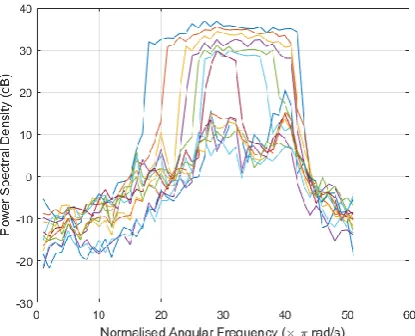
After performing the MSME-SMD PEVD [13] algorithm on the spatially smoothed covariance matrix from (17), the dimensions of the eigenspaces is determined by the number of significant eigenvalues. This can be done in two ways, the first being evaluating the polynomial eigenvalues to estimate their power spectral density and analysing the peak magnitude over a certain threshold, as demonstrated in Figure 1.

Figure 1: Polynomial Eigenvalue PSD for the Co-Prime Method

[image:5.595.312.531.76.232.2]

5

Figure 2: Summed Polynomial Eigenvalue Coefficients for the Co-prime array

The former contains information of the power spectral density of the sources in addition to the number of significant eigenvalues. The latter is however clearer and is the same representation as the conventional eigenvalue plot.

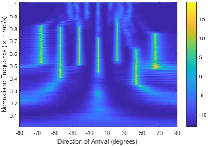
Since our spatially smoothed virtual space time covariance matrix has dimensions 𝑹̂ (𝑧)𝑥𝑥 ∈ 𝐶𝑀𝑁+1×𝑀𝑁+1(𝑧), thus the noise sub space is 𝑼 (𝑧)𝑛 ∈ 𝐶𝑀𝑁+1−𝑃×𝑀𝑁+1(𝑧) dimensional. Performing the SSP-MUSIC algorithm on the estimated noise subspace produces the spatio-spectrum seen in Figure 3.

Figure 3: Co-prime SSP-MUSIC performance

From the very sharp peaks in this spatio-spectrum, the estimated frequencies and directions of arrival from Table 1 are correctly estimated in Figure 3. The sharp peaks are due to the super resolution property of these subspace based methods.

6.2

Conventional ULA SSP-MUSIC Algorithm

[image:5.595.53.277.77.231.2]

A ULA comprising of 21 elements yields the same physical length as the co-prime array. The sum of polynomial eigenvalues of the space-time covariance for this very long uniform linear array can be seen in Figure 4.

Figure 4: Summed Polynomial Eigenvalue Coefficients for the ULA

The seven significant eigenvalues are very clear from both the magnitude and gradient change of the eigenvalues, determining the size of the signal and noise subspaces. The SSP-MUSIC algorithm was performed on the polynomial noise subspace, and the results are displayed in Figure 5.

Figure 5: Conventional 21 Element ULA SSP-MUSIC performance

The co-prime and conventional uniform linear array approach both result in very similar estimates of the spatio spectrum. The peaks are noticeably sharper in the conventional ULA approach. One of the reasons is that the 21 element ULA based approach required 2.3 times the number of antenna elements to yield the same physical aperture for the co-prime array used in this simulation. Due to the spatial smoothing scheme used for the co-prime approach, some virtual aperture was lost to decorrelating the sources. Thus the ULA based approach had the benefit of a higher dimensional noise subspace. Nevertheless, this minor trade-off in performance comes with the major benefit of a significantly reduced number of sensors.

7 Conclusion

[image:5.595.315.529.362.512.2] [image:5.595.56.268.427.577.2]

6

performance and compare to a uniform linear array with the same physical aperture. We note that the both methods perform similarly, with the co-prime method utilising a significant reduction in antenna elements required. Results demonstrate a promising solution to reducing the number of sensors required in a wideband antenna array with little sacrifice in performance.

Acknowledgement

This work was supported by Leonardo MW Ltd and EPSRC grant number EP/N509760/1.

References

[1] Y. Jia, X. Zhong, Y. Guo, and et al. “DoA and DoD estimation based on bistatic mimo radar with co-prime array” In 2017 IEEE Radar Conference (RadarConf), pages 0394– 0397, May 2017.

[2] R. Schmidt. “Multiple emitter location and signal parameter estimation” IEEE Trans. Antennas and Propagation, 34(3):276–280, Mar 1986.

[3] R. Roy and T. Kailath. “Esprit-estimation of signal parameters via rotational invariance techniques” IEEE Transactions on Acoustics, Speech, and Signal Processing, 37(7):984–995, Jul 1989.

[4] Piya Pal and P. P. Vaidyanathan. “Coprime sampling and the music algorithm” 2011 Digital Signal Processing and Signal Processing Education Meeting, DSP/SPE 2011 - Proceedings, 0(1):289–294, 2011.

[5] J. E. Evans, J. R. Johnson, and D. F. Sun. “Application of advanced signal processing techniques to angle of arrival estimation in atc navigation and surveillance system” 1982.

[6] Tie-Jun Shan, M. Wax, and T. Kailath. “On spatial smoothing for direction-of-arrival estimation of coherent signals” IEEE Trans. Acoustics, Speech, and Signal Processing, 33(4):806–811, Aug 1985.

[7] S Weiss, S Bendoukha, A Alzin, et al "MVDR broadband beamforming using polynomial matrix techniques," 2015 23rd European Signal Processing Conference (EUSIPCO), Nice, 2015, pp. 839-843.

[8] M. A. Alrmah, S. Weiss, and S. Lambotharan. “An extension of the music algorithm to broadband scenarios using a polynomial eigenvalue decomposition” In 2011 EUSIPCO, pages 629–633, Aug 2011.

[9] William Coventry, Carmine Clemente, and John Soraghan. “Enhancing Polynomial MUSIC Algorithm for

Coherent Broadband Sources Through Spatial Smoothing” In EUSIPCO 2017, pages 2517–2521, 2017.

[10] P. P. Vaidyanathan and Piya Pal. “Sparse Sensing With Co-Prime Samplers and Arrays” IEEE Transactions on Signal Processing, 59(2):1405–1409, 2010.

[11] J. G. McWhirter, P. D. Baxter, T. Cooper et al. “An evd algorithm for para-hermitian polynomial matrices” IEEE Trans. Signal Processing, 55(5):2158–2169, May 2007.

[12] S. Redif, S. Weiss, and J. G. McWhirter. “Sequential matrix diagonalization algorithms for polynomial evd of parahermitian matrices” IEEE Trans. Signal Processing, 63(1):81–89, Jan 2015.

[13] J. Corr et al. Multiple shift maximum element

sequential matrix diagonalisation for parahermitian matrices. In 2014 IEEE Workshop on Statistical Signal Processing (SSP), pages 312–315, June 2014.

[14] J. Corr, K. Thompson, S. Weiss et al. Shortening of paraunitary matrices obtained by polynomial eigenvalue decomposition algorithms. In 2015 Sensor Signal Processing for Defence (SSPD), pages 1–5, Sept 2015.

[15] F. K. Coutts, K. Thompson, I. K. Proudler et al. “A comparison of iterative and dft-based polynomial matrix eigenvalue decompositions” In 2017 IEEE 7th International Workshop on Computational Advances in Multi-Sensor Adaptive Processing (CAMSAP), pages 1–5, Dec 2017.

[16] F. Coutts, K. Thompson, S. Weiss et al. “Impact of fast-converging PEVD algorithms on broadband AoA estimation” In 2017 Sensor Signal Processing for Defence Conference (SSPD), pages 1–5, Dec 2017.

[17] M. Alrmah, S. Weiss, and J. McWhirter.