City, University of London Institutional Repository
Citation
:
Chitsanga, N., Giaralis, A. ORCID: 0000-0002-2952-1171 and Kaitwanidvilai, S. (2018). Robust cascade H infinity control of BLDC motor systems using fixed-structure two degrees of freedom controllers designed via genetic algorithm. Paper presented at the International MultiConference of Engineers and Computer Scientists 2018, 14-16 Mar 2018, Kowloon, Hong Kong.This is the published version of the paper.
This version of the publication may differ from the final published
version.
Permanent repository link: http://openaccess.city.ac.uk/21908/
Link to published version
:
Copyright and reuse:
City Research Online aims to make research
outputs of City, University of London available to a wider audience.
Copyright and Moral Rights remain with the author(s) and/or copyright
holders. URLs from City Research Online may be freely distributed and
linked to.
City Research Online: http://openaccess.city.ac.uk/ [email protected]
Abstract— A robust control technique is proposed to
regulate the current and angular velocity in typical brushless direct current (BLDC) motors. The proposed technique relies on two degree-of-freedom (2-DOF) H infinity control with loop shaping in which the structure of the two controllers and the loop shaping function are pre-specified parametrically (i.e., attain a fixed-structure). This consideration allows for striking a desirable balance between control effectiveness and controllers’ simplicity safeguarding feasibility of practical implementation. It further allows for using standard genetic algorithm (GA) for searching optimal controller parameters. Herein, two 2-DOF fixed-structure H infinity control structures are used in cascade to regulate BLDC motor response in time and in frequency domain subject to internal and external disturbances. Simulation results pertaining to a model of a particular commercial BLDC motor derived through standard system identification demonstrate the applicability and robustness of the proposed control technique to changes to internal BLDC resistance and external BLDC payload. It is shown that the proposed technique is more robust than optimal cascade 1-DOF PID control treated as a special case of the proposed technique.
Index Terms—2-DOF H-infinity control, BLDC motor
system, genetic algorithm, Fixed-structure control, robust control and cascade control
I. INTRODUCTION
rushless direct current (BLDC) motors have been increasingly popular across industrial sectors as they enjoy significant advantages over other types of ac and dc motors such as higher power density, simpler manufacturing and lower production cost. Therefore, developing dependable controllers for BLDCs is a timely issue and an area of open research [1]. To this aim, this paper considers robust H-infinity speed control of typical BLDC motors by adopting a recently developed by the first and third author strategy for designing two degree-of-freedom (2-DOF) robust controllers [2,3]. The adopted strategy considers parametrically defined fixed-structure 2-DOF controllers with loop-shaping to safeguard simplicity and feasibility in
N. Chitsanga and S. Kaitwanidvilai are with the Faculty of Engineering, King Mongkut's Institute of Technology Ladkrabang, Bangkok 10520, Thailand. Email: [email protected] and [email protected].
A. Giaralis is with the School of Mathematics, Computer Science & Engineering, City, University of London, London, EC1V 0HB, UK. E-mail : [email protected]
practical realization and uses genetic algorithm (GA) search to achieve optimality in design [4,5]. The effectiveness and applicability of the above strategy for robust H-infinity control has been previously demonstrated for the case of dc motors [2,3]. In particular, superior robustness has been achieved in both time and frequency domain compared to 1-DOF PID controllers.
Herein, the above fixed-structure 2-DOF control strategy with loop-shaping is extended to treat the case of BLDC motors by introducing a cascade control structure comprising two 2-DOF controllers in series. In this manner, both the angular velocity and the current within the BLDC are simultaneously controlled. The controllers are of low-order due to the fixed-structure design approach and their parameters are optimized by means of GA. For numerical illustration, a commercial BLDC motor is considered and represented by transfer functions derived by solving a system identification problem against simulated data. The BLDC motor model is controlled by the proposed cascade 2-DOF controllers at a specific nominal speed. Cascade 1-DOF PID H-infinity controllers are also derived as a special case using the same fixed-structure design strategy and their performance is compared to the 2-DOF controller. Both cascade 2-DOF and 1-DOF controllers are tested for robustness against external and internal disturbances.
The remainder of the paper is organized in five sections. Section II presents the state-space equations of standard BLDC motor and derives pertinent transfer functions via a standard system identification approach pertaining to a particular of-the-shelve device. Section III reviews the adopted fixed-structure 2-DOF H-infinity control approach using GA and discusses its extension to a cascade configuration tailored for BLDC motor control. It further provides illustrative numerical results to support its applicability for the device considered in the previous Section. Next, Section IV furnishes comparative simulation-based data demonstrating the performance of the cascade 2-DOF control approach vis-à-vis cascade 1-2-DOF control. Lastly, Section V summarizes concluding remarks.
II. THE DYNAMIC MODEL OF BLDC MOTOR SYSTEM
A. State-space representation of BLDC motor system The standard three-phase BLDC motor system can be represented in state-space by the equations [6]
Robust Cascade H Infinity Control of BLDC
Motor Systems using Fixed-Structure Two
Degrees of Freedom Controllers Designed Via
Genetic Algorithm
N. Chitsanga, A. Giaralis and S. Kaitwanidvilai
where is the 4-by-4 identity matrix and
;
;
;
;
(2)
In the above expressions, ias, ibs and ics are the current of
stator per phase of the BLDC motor; ωm is the angular
velocity; Vas, Vbs and Vcs are the voltage input per phase; TL
is the torque of the mechanical load; Rs is the resistance per
phase; L1=L-M, where L is the self-inductance per phase
common for all three phases and M is the common mutual inductance between phases; J is the rotational inertia; B is the flux density of the magnetic field; kt is the torque
constant; and kv is the velocity constant. The above
state-space representation is used in the following system identification step to model a commercial BLDC motor operating with a common current and voltage across the three phases. That is, ias =ibs=ics = i and Vas= Vbs = Vcs=V.
B. System identification of a specific BLDC motor The electromagnetic torque produced by a BLDC motor is given by the product of the torque constant times the stator current [7]. That is, . Moreover, the
electromotive force of the motor is given by the product of the velocity constant times the angular velocity [6]. That is,
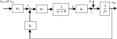
. In this regard, Fig.1 provides a block diagram
of a typical BLDC motor in which two weighting functions, W1 and W2, are also included to achieve loop shaping. These
two constants are acting as pre-compensator weight functions and are determined using the genetic algorithm (GA) approach discussed in the following section. Setting for the time being W1=W2=1, the following transfer
functions are obtained based on the BLDC system of Fig.1
and
(3)
where ωref is the input/excitation signal in terms of angular
[image:3.595.69.291.83.218.2]velocity.
Fig. 1. Block diagram of BLDC motor system with loop shaping weighting functions.
is used to illustrate the proposed control strategy described in the following section. This motor has been previously examined in [7] and is characterized by the following properties kt = 25.1 mN.m/A; kv = 380 r/min/V; R = 0.454
kOhm; J = 135 g.cm2; L = 0.322 mH. It is then sought to represent the above motor by surrogate linear dynamic models that can faithfully predict response motor data as obtained by numerical integration of (1) for a test input signal u (excitation). To this aim, the standard output error (OE) method of system identification [8] is herein considered to determine the coefficients f1, f2,…, fnfand b1 , b2 , …, bnbof pertinent transfer functions defining the sought
linear models in the form of
(4)
In the above equation nf and nb are the number of poles and zeros, respectively, of the transfer function. It is seen from (3) that the overall BLDC system has two poles and no zero. By application of the OE method, as visualized in Fig. 3, the coefficients in (4) are determined assuming nf = nb +1 =2
and delay equal to 1 such that the error of the sought models compared to simulation results from (1) is minimized in the mean sense for reference input
and . (5)
The resulting models read as
and
(6)
[image:3.595.368.488.543.590.2]and are used in the remainder of the paper to represent a typical BLDC motor.
Fig 2. Block diagram of Output Error model.
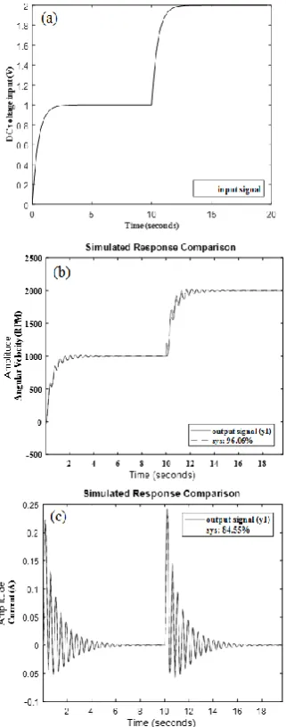
To illustrate the quality of the applied system identification step, Fig. 3(a) plots the DC voltage input and Fig. 3(b) and 3(c) plot the output signals in terms of angular velocity and current, respectively, obtained from (1) and from the identified models. The normalized root mean square error is reported as a measure for the achieved goodness of fit.
W2 W1
kt
kv
+
- +
- ωm
TL
[image:3.595.51.297.650.733.2]Fig 3. The output error of system identification on BLDC motor system (a) input signal (b) angular velocity model (c) current model
III. OPTIMAL H INFINITY CONTROL OF BLDC MOTORS
A. Fixed-structure 2-DOF H-infinity control using GA A 2-DOF H-infinity control strategy with loop-shaping [9] is herein adopted for regulating the response of a given dynamical system (i.e., “plant”) with nominal transfer function G. This control strategy comprises a feed-forward controller, Kp, regulating time-domain response of the
closed-loop system and a feedback controller, Kq, designed
to ensure robust stability of the system to plant model uncertainty and to disturbances (see Fig. 4). In this setting, time-domain specifications are defined through a reference model, Tref. Further, the scalar ρ leverages the significance in
satisfying the time-domain specifications governed by Tref
[image:4.595.93.254.52.461.2]during solution of the optimal control design problem. Lastly, loop-shaping is achieved by considering a pre-compensating weight function W which, in Fig. 4, is absorbed within the two controllers.
Fig 4. Standard 2-DOF control scheme with loop-shaping.
For design purposes, the transfer function Gs of the plant
is shaped by the use of W and can be written with the aid of co-prime factors as [10]
Gs=GW=Ms-1Ns (7)
where Ns and Ms are the numerator and the denominator
factor, respectively. By adopting the modified plant Gs in
(7), the sought optimal controllers become
Kp∞= W-1 Kp and Kq∞= W-1 Kq. (8)
Further, uncertainty to the plant system is introduced through the model shown in Fig. 5. The transfer function of the uncertain plant becomes
G∆=(Ns+∆Ns)(Ms+∆Ms)-1, (9)
where ∆Ns and ∆Ms are unknown bounded modeling
perturbations of the numerator and denominator, respectively, of the plant transfer function such that
|∆Ns, ∆Ms|∞ ≤ ε, (10)
where ε is a stability margin and |∙|∞ is the standard infinity
norm.
Fig 5. Uncertainty plant system model using co-prime factorization.
Application of conventional optimal robust control design for the above uncertain system typically yields high-order controllers which may be difficult to realize in practical applications [4,5]. This problem can be overcome by pre-specifying parametrically the structure of the two controllers as well as of the shaping function as discussed in [3-5]. Standard GA can further be used to search optimal parameters for the fixed-structure Kp∞, Kq∞, and W
[image:4.595.304.546.488.594.2]fixed-structure parameters for the shaping function and for the controllers Kp and Kq, respectively.
Step 2: The reference model Tref is specified defining the
desired time-domain specifications for the controlled system to satisfy. Further, a value for the design scalar parameter ρ in Fig.4 is selected. Note that by setting ρ=0, the 2-DOF control scheme in Fig.4 degenerates to a standard 1-DOF scheme with a single controller Kq.
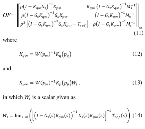
Step 3: The objective function is constructed [9]
OF
(11) where
(12)
and
(13)
in which is a scalar given as
(14)
The last “zero-frequency” (dc) factor is the required gain to ensure that the targeted amplitude of the optimally controlled system is compatible with the amplitude of the reference model in time-domain. The terms in (11) are associated with different desired performance requirements as detailed in [9].
Step 4: GA is used [11] to search for the parameters pw,
pp, andpq simultaneously that minimize the norm in (11).
That is, to solve the minimization problem
(15)
where p is a vector collecting all design variables (i.e., all elements of vectors pw, pp, andpq), and pmin and pmax are
vectors collecting pre-specified lower and upper allowed values of the design parameters defining the design space. The optimal stability margin is computed as
(16)
which can be treated as a quality index for the optimal design solution achieved through the use of GA (see also [10]).
B. Proposed cascade fixed-structure 2-DOF robust control for BLDC motors
The previously described 2-DOF H-infinity control strategy with fixed-structure controllers and loop-shaping function is herein used to control both the output angular
considered in series, as shown in Fig. 6. The inner control structure regulates the current of the BLDC motor; it comprises controllers K1and K2 operating on “plant 1” as
identified in Fig.6. The outer control structure regulates the angular velocity of the BLDC motor; it comprises controllers K3and K4 operating on “plant 2” as identified on
[image:5.595.309.540.174.265.2]the same figure.
Fig 6. Diagram of proposed cascade 2-DOF control for BLDC motors
Optimal controller design for the proposed cascade 2-DOF H infinity control strategy is accomplished by applying sequentially and independently twice the steps listed in the previous sub-section. Specifically, the above steps are applied once to optimally design the controllers K1 and K2.
In doing so, G is replaced by G1 in (7), Tref in (11) and (14)
becomes iref and the subscripts “p” and “q” are replaced by
subscripts “1” and “2” in (11)-(14), respectively. Upon optimal design of K1 and K2, controllers K3 and K4 are next
designed by a second application of the same steps in which G is replaced by G2G1K1/(1-G1K2) in (7), Tref in (11) and
(14) becomes ωref and the subscripts “p” and “q” are
replaced by subscripts “3” and “4” in (11)-(14), respectively. An illustrative optimal design example of the proposed cascade 2-DOF control strategy is provided in the following section for the particular BLDC model shown in Fig.1 and defined in (5) and (6) with numerical assessment for robustness.
As a closure to this section, it is noted that the proposed optimal design procedure for cascade 2-DOF H infinity control degenerates to cascade 1-DOF PID H infinity control shown in Fig.7 by setting ρ=0 in (11) and by choosing a PID parametric form (structure) for the two remaining controllers K2 and K4 denoted by KPID1 and KPID2,
[image:5.595.42.293.204.426.2]respectively, in Fig.7. In the following section an example of an optimally designed cascade 1-DOF PID H infinity control with numerical assessment for robustness is also provided for the BLDC model in (5) and (6) to compare its effectiveness vis-à-vis the herein proposed cascade 2-DOF control.
[image:5.595.306.549.673.750.2]IV. OPTIMAL CONTROL DESIGN AND NUMERICAL ASSESSMENT VIA SIMULATION
A. Illustrative optimal design application of proposed cascade fixed-structure 2-DOF H-infinity control
In this section the model of the commercial BLDC motor derived through system identification in II.B is considered to exemplify the cascade fixed-structure 2-DOF H infinity robust control strategy in Fig.6 and its optimal design. For the sake of comparison, a second cascade fixed-structure 1-DOF H infinity control shown in Fig. 7 (i.e., a special case of the cascade 2-DOF control strategy) is also pursued. The nominal plant transfer functions in Figs. 6 and 7 read as
and . (17)
For the cascade 2-DOF control, the following parametric forms are assumed for W1, K1, and K2 (inner control
structure) and for W2, K3, and K4(outer control structure)
and , (18)
and
, (19)
and
. (20)
For the cascade 1-DOF PID control, the following parametric forms are assumed for W11 and KPID1 (inner
control structure) and for W22, and KPID2 (outer control
structure)
, (21)
, (22)
and
. (23)
Note that K2and K4 are purposely chosen to attain a PID
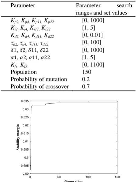
form to support a meaningful comparison with the cascade 1-DOF PID case. Note also that the shaping function is chosen to have the same form for all control structures. Table 1 reports the pre-specified search range for each parameter entering the definition of the parametric forms in (18)-(23) which define the pmin and pmax vectors in the
optimal search through GA in (15) as well as pertinent values for parameters associated with GA implementation [14].
Further, Fig. 8 plots the average optimal stability margin as a function of the population number used in the GA from the two optimization problems solved (one for the inner and one for the outer control structures) in the cascade 2-DOF control case. It is seen that convergence is achieved swiftly. Lastly, Table 2 collects the results of optimal parametric searching through GA for both 2-DOF and 1-DOF PID control cases.
TABLE 1.THE BOUNDARY CONDITION OF PARAMETERS FOR
GENETIC ALGORITHM OPTIMIZATION
Parameter Parameter search ranges and set values Kp2, Kp4, Kp11, Kp22 [0, 1000]
Ki2, Ki4, Ki11, Ki22 [1, 5] Kd2, Kd4, Kd11, Kd22 [0, 0.01]
d2,d4,d11,d22 [0, 100] , [0, 1000]
, [1, 5] Kf1, Kf3 [0, 1100]
Population 150
Probability of mutation 0.2 Probability of crossover 0.7
Fig 8. Average optimal stability margin achieved for robust 2 DOF and cascade control
TABLE 2. OPTIMAL WEIGHTING FUNCTIONS, CONTROLLERS AND STABILITY MARGIN OF 2-DOF AND 1-DOF CONTROL CASES.
1DOF control 2DOF control
weighting function
controller
Average stability margin
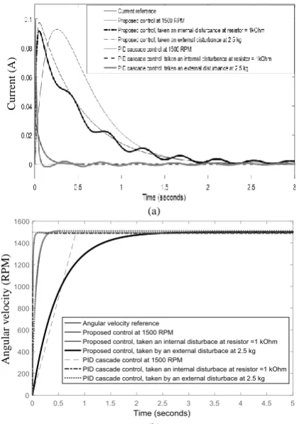
[image:6.595.314.540.72.373.2] [image:6.595.48.291.294.377.2] [image:6.595.298.554.445.686.2]For assessment, the adopted BLDC motor model is assumed to operate at 1500rpm. Figure 7 plots the response of the optimally designed control strategies of Table 2 vis-à-vis the reference response in terms of current (Fig. 7(a)) and in terms of angular velocity (Fig. 7(b)) for this speed. Further, Table 3 reports the control performance in terms of rise time (RT), settling time (ST), and overshoot (O), as computed through the simulated response data. It is seen that the BLDC controlled by the optimally designed cascade 2-DOF control strategy traces closer the desired response compared to the BLDC with cascade 1-DOF control. This is particularly true for the ST which is significantly closer to the reference compared to the 2-DOF control case for both BLDC current and angular velocity.
Moreover, the robustness of the optimally controlled BLDC for both 2-DOF and 1-DOF control cases is tested to internal and external disturbances applied independently. The internal disturbance is modelled through a change to the resistance R of the BLDC motor from the nominal 0.454 to 1 kOhm. The external disturbance is a torque input given by 1/2500s2 in the Laplace domain corresponding to 2.5kg of proof mass. Figure 7 superposes simulated responses of optimally designed 2-DOF and 1-DOF PID controlled BLDC to the above disturbances, while Table 3 reports RT, ST, and O data as before. It is found that the 2-DOF control strategy is evidently more robust to 1-DOF PID control as it traces closer the desired output subject to disturbance. Robust performance is significantly different for the internal disturbance which is the critical since it corresponds to a large change of the internal resistance.
V. CONCLUDING REMARKS
A robust cascade 2-DOF fixed-structure H infinity control approach with loop shaping has been proposed and applied to regulate the response of a typical BLDC motor in terms of current and angular velocity. The approach allows for striking a good balance between control effectiveness and controllers’ simplicity safeguarding feasibility of practical implementation. It further allows for using standard genetic algorithm (GA) for searching optimal controller parameters which readily automates the optimal design process of the 4 required controllers. Simulation results pertaining to a model of a particular commercial BLDC motor derived through standard system identification demonstrated the applicability and robustness of the proposed control technique to changes to internal BLDC resistance and external BLDC torque load. It has been further shown that the proposed technique is more robust than optimal cascade 1-DOF PID control herein treated as a special case. Overall, based on the herein reported numerical results, the proposed control approach and optimal design procedure is a valid and viable solution that can be considered for controlling BLDC motors in various industrial applications.
(a)
(b)
Fig 7. The response of both controls at speed 1500 RPM and tested the robustness by taken internal and external disturbance.
(a) Current response (b) Angular velocity response
TABLE 3. THE DYNAMIC RESPONSES OF THE PROPOSED CONTROL AND 1DOF CASCADE CONTROL ON BLDC MOTOR
Proposed cascade 2-DOF control
Cascade 1-DOF PID control RT(s) ST(s) O(%) RT(s) ST(s) O(%)
iref 0.01 1.87 9.28 0.01 1.87 9.28
i at 1500rpm 0.01 1.83 9.19 0.01 0.34 9.92
i at 1kOhm 0.01 1.90 9.76 0.01 0.23 3.15
i at 2.5kg. 0.01 1.83 9.19 0.01 0.34 9.92
ωref 0.05 1.89 0 0.05 1.89 0
ω at 1500rpm 0.05 1.89 0 0.08 0.82 0
ω at 1kOhm 0.05 1.89 0 3e-4 0.05 0
ω at 2.5kg. 0.05 1.89 0 5e-4 0.26 0
ACKNOWLEDGEMENTS
This work was supported by the King Mongkut’s Institute of Technology Ladkrabang, City, University of London and also by doctoral student scholarship under the Research and Researcher Industry (RRi), the Thailand Research Fund (PHD58I0091).
Cu
rr
en
t (
A
)
An
g
u
lar
v
elo
city
(
[image:7.595.323.534.51.350.2] [image:7.595.301.554.459.577.2]REFERENCES
[1] Gamazo-Real JC, Vázquez-Sánchez E, Gómez-Gil J. Position and Speed Control of Brushless DC Motors Using Sensorless Techniques and Application Trends. Sensors 2010;10(7):6901-6947. doi:10.3390/s100706901.
[2] N. Chitsanga and S. Kaitwanidvilai, “Robust 2DOF fuzzy gain scheduling control for DC servo speed controller," IEEJ Transactions on Electrical and Electronic Engineering, vol.11 no.6, 2016.N. [3] Chitsanga and S. Kaitwanidvilai, “Robust DC Motor System and
Speed Control Using Genetic Algorithms with Two Degrees of Freedom and H Infinity Control,” WCECS, vol. 2, pp. 792-796, 2017. [4] S. Kaitwanidvilai, P. Olranthichachat and Manukid Parnichkun, “Fixed Structure Robust Loop Shaping Controller for a Buck-Boost Converter using Genetic Algorithm,” IMECS, vol. 2, pp. 1511-1516, 2008.
[5] Nuttapon Phurahong, Somyot Kaitwanidvilai and Atthapol Ngaopitakkul, “Fixed Structure Robust 2DOF H-infinity Loop Shaping Control for ACMC Buck Converter using Genetic Algorithm,” IMECS, vol. 2, pp. 1030-1035, 2012.
[6] Snehasree R. S., “Modeling of Permanent Magnet BLDC Motor Using State Space Analysis,” International Journal of Innovative Research & Development, vol.2 no.6, 2013.
[7] A. Darba, F. D. Belie, P. D. haese, and J. A. Melkebeek, “Improved Dynamic Behavior in BLDC Drives Using Model Predictive Speed and Current Control,” IEEE Transactions on Industrial Electronics, vol. 63, pp. 728-740, 2016.
[8] Ljung L., System Identification: Theory for the User 2nd edition. New Jersey: Prentice-Hall, 1999.
[9] Hoyle, D.J., Hyde, R.A. and Limebeer, D,J.N., “An Η∞ approach to two degree of freedom design”, Proceedings of the 30th IEEE Conference on Decision and Control, Vol. 2, 1581-1585, 1991. [10] McFarlane Duncan and Glover Keith, “A loop shaping design
procedure using H∞ synthesis,” IEEE Transactions on automatic
control, vol. 37, no. 6, pp. 759-769, 1992.
[11] S. Kaitwanidvilai and M. Parnichkun, “Genetic algorithm based fixed-structure robust Η∞ loop shaping control of a pneumatic servo