City, University of London Institutional Repository
Citation
: Endress, A. and Langus, A. (2017). Transitional probabilities count more than
frequency, but might not be used for memorization. Cognitive Psychology, 92, pp. 37-64. doi:
10.1016/j.cogpsych.2016.11.004
This is the accepted version of the paper.
This version of the publication may differ from the final published
version.
Permanent repository link:
http://openaccess.city.ac.uk/15795/
Link to published version
: http://dx.doi.org/10.1016/j.cogpsych.2016.11.004
Copyright and reuse:
City Research Online aims to make research
outputs of City, University of London available to a wider audience.
Copyright and Moral Rights remain with the author(s) and/or copyright
holders. URLs from City Research Online may be freely distributed and
linked to.
City Research Online:
http://openaccess.city.ac.uk/
[email protected]
Transitional probabilities count more than frequency, but might not be
used for memorization
Ansgar D. Endress
Department of Psychology, City, University of London, UK
Alan Langus
Cognitive Neuroscience Sector, International School for Advanced Studies, Trieste, Italy
Learners often need to extract recurring items from continuous sequences, in both vision and audition. The best-known example is probably found in word-learning, where listeners have to determine where words start and end in fluent speech. This could be achieved through universal and experience-independent statistical mecha-nisms, for example by relying on Transitional Probabilities (TPs). Further, these mechanisms might allow learners to store items in memory. However, previous in-vestigations have yielded conflicting evidence as to whether a sensitivity to TPs is diagnostic of the memorization of recurring items. Here, we address this issue in the visual modality. Participants were familiarized with a continuous sequence of visual items (i.e., arbitrary or everyday symbols), and then had to choose between (i) high-TP items that appeared in the sequence, (ii) high-TP items that did not appear in the sequence, and (iii) low-TP items that appeared in the sequence. Items matched in TPs but differing in (chunk) frequency were much harder to discriminate than items differing in TPs (with no significant sensitivity to chunk frequency), and learners preferred unattested high-TP items over attested low-TP items. Contrary to previous claims, these results cannot be explained on the basis of the similarity of the test items. Learners thus weigh within-item TPs higher than the frequency of the chunks, even when the TP differences are relatively subtle. We argue that these results are problematic for distributional clustering mechanisms that analyze continuous sequences, and provide supporting computational results. We suggest that the role of TPs might not be to memorize items per se, but rather to prepare learners to memorize recurring items once they are presented in subsequent learning situations with richer cues.
Introduction
In many situations, we need to extract recurring units from continuous sequences. For example, we move con-tinuously through space, but can separate the continu-ous motion into discrete actions (e.g., Newtson, 1973; Newtson, Engquist, & Bois, 1977; Zacks & Tversky, 2001; Zacks & Swallow, 2007). We can recognize motifs from hour-long symphonic works, and, while navigat-ing, we experience a sequence of visual snapshots (e.g., of landmarks), that we can retrieve as a sequence from
ADE was supported by grant PSI2012-32533 from Spanish Ministerio de Econom´ıa y Competitividad and Marie Curie Incoming Fellowship 303163-COMINTENT. We thank Fer-nando Genestar and Neus Colomer for assistance with data collection, and Antonia Stanojevi´c for helpful comments on an earlier version of this manuscript. Contributions: ADE designed, implemented and analyzed the studies. Both au-thors contributed to the writing of the manuscript.
memory when we try to take the same trajectory again.
This class of problems has been studied most exten-sively in the context of language acquisition. To compe-tent adult listeners, fluent speech seems to be composed of a discrete sequence of words, much as words are sep-arated by white space in written text. However, fluent speech does not comprise the equivalent of white space. Hence, before infants can learn the meaning of any word, they first have to isolate them from fluent speech, and learn where words start and where they end. This prob-lem is called the segmentation probprob-lem.
there is substantial evidence that human adults, infants and other animals are sensitive to TPs in a variety of modalities, including language and the visual modality (see, among many others, Aslin, Saffran, & Newport, 1998; Creel, Newport, & Aslin, 2004; Endress, 2010; En-dress & Wood, 2011; Fiser & Aslin, 2002a, 2005; Glick-sohn & Cohen, 2011; Hauser, Newport, & Aslin, 2001; Saffran, Newport, & Aslin, 1996; Saffran, Aslin, & New-port, 1996; Saffran, Johnson, Aslin, & NewNew-port, 1999; Saffran & Griepentrog, 2001; Toro & Trobal´on, 2005; Turk-Browne, Jung´e, & Scholl, 2005; Turk-Browne & Scholl, 2009), studies assessing whether the output of TP computations is stored in memory have yielded con-flicting results (see below). Moreover, the degree to which TPs lead to memorization seems to depend on the participants’ native language (see Endress & Mehler, 2009b; Langus & Endress, under review; Perruchet & Poulin-Charronnat, 2012, and below).
Here, we ask whether visual TPs provide segmented chunks that can be memorized. We use visual stimuli for two reasons. First, given that speakers of different languages behaved differently in previous experiments (Endress & Mehler, 2009b; Langus & Endress, under re-view; Perruchet & Poulin-Charronnat, 2012), we sought to investigate this issue in a domain that is unlikely to be influenced by prior knowledge of one’s native language, and might thus give a relatively uncontaminated pic-ture of how statistical learning operates in the absence of language-specific knowledge. Second, it is unknown whether statistical learning of visual sequences leads to memorization (though there is some evidence on this issue for spatial visual arrays; see below). This issue is important because statistical learning abilities seem rel-atively uncorrelated across domains (Frost, Armstrong, Siegelman, & Christiansen, 2015; Garcia, Hankins, & Rusiniak, 1974; Siegelman & Frost, 2015), and might, in some cases, have different properties in different do-mains.
The question of whether statistical learning leads to memorization of units also touches on a second im-portant question: How do statistical learning mecha-nisms operate? In the word segmentation literature, two important classes of mechanisms have been proposed: bracketing and clustering (Goodsitt, Morgan, & Kuhl, 1993; see also Thiessen, Kronstein, & Hufnagle, 2013, for a review). Bracketing operates by inserting bound-aries between words, and thus presumably requires addi-tional mechanisms to place items in memory. Clustering mechanisms, in contrast, chunk syllables together, and thus create units that can be memorized directly. To use a visual analogy, letters that are part of the same word have two related properties: they have at least one spatially adjacent letter (unless they are single
let-ter words), and they are adjacent to at most one white space or punctuation element. In principle, either prop-erty might be sufficient to find word boundaries: one can infer where words start or end by monitoring the statistical cohesiveness of the statistics within a chunk of letters (clustering), or one could posit the start of a new word once a boundary cue (such as white space) is encountered (bracketing). However, the distinction between bracketing and clustering has rarely been ad-dressed in the visual modality.
Below, we will first ask whether statistical learning of visual sequences leads to memorization of recurring units. Based on these and earlier results, we will then provide general arguments and illustrative simulations to show that these results are problematic for distribu-tional chunking mechanisms.
Statistical learning of recurring sequences
The most widely researched strategy to extract re-curring units from sequences relies on distributional cues, notably on transitional probabilities (TPs). In the speech domain, TPs reflect the conditional proba-bility of one syllable σ1 following another syllable σ2: P(σ2|σ1) = P(σ1σ2)/P(σ1), where σ1σ2 is a syllable string. For example, Saffran, Aslin, and Newport (1996) showed that seven-months old infants can track TPs across syllables. Specifically, infants were exposed to a concatenation of made-up words. As a result, sylla-bles within words had high TPs, while syllasylla-bles span-ning a word-boundary had relatively lower TPs. In-fants discriminated high-TP items from low-TP items. Following this seminal paper, there has been a wealth of demonstrations that infants and also non-human an-imals are sensitive to TPs not only for speech mate-rial, but also for a variety of other stimuli (Creel et al., 2004; Endress, 2010; Fiser & Aslin, 2001, 2002b; Hauser et al., 2001; Saffran, Aslin, & Newport, 1996; Saffran et al., 1999; Toro & Trobal´on, 2005; Turk-Browne et al., 2005). Further, the idea that distributional cues in a variety of guises might be used for extracting re-curring sequences has been implemented in numerous computational models (e.g., Batchelder, 2002; Brent & Cartwright, 1996; Christiansen, Allen, & Seidenberg, 1998; Frank, Goldwater, Griffiths, & Tenenbaum, 2010; Orb´an, Fiser, Aslin, & Lengyel, 2008; Perruchet & Vin-ter, 1998; Swingley, 2005).1
1This is not to say that statistical learning is the only
Statistical learning and memory
To learn recurring sequences, learners must have a way to place them in memory. While this condition has rarely been discussed in the literature (see Endress & Mehler, 2009b; Endress & Hauser, 2010), it is more constraining than it seems. For example, with speech items, participants are not only sensitive to forward TPs, but also to backward TPs (Perruchet & Desaulty, 2008; Pelucchi, Hay, & Saffran, 2009). That is, in a syllable sequenceσ1σ2, participants are not only sensi-tive to TPs of the formP(σ2|σ1), but also to TPs of the form P(σ1|σ2). Moreover, at least in vision, if partic-ipants are familiarized with a sequence ABC, they are as good at recognizing ABC asCBA(Endress & Wood, 2011; Turk-Browne & Scholl, 2009). Unless one assumes that participants also memorize theCBAsequences al-though they never see them, it appears that successful discrimination of high-TP items from low-TP items does not imply that the high-TP items have been memorized. For example, a representation of a syllable or of a visual item might form associations with other representations of such items. However, in contrast to what is generally assumed in the segmentation literature, the representa-tions that end up being associated with each other might not be integrated into a single memory representation.
At first sight, these conclusions seem to be con-tradicted by Graf-Estes, Evans, Alibali, and Saffran’s (2007) results (see also Hay, Pelucchi, Graf Estes, & Saffran, 2011). These authors familiarized infants with a continuous speech stream that contained nonsense words defined by TPs. Following this familiarization, infants had to associate visual images with words (i.e., high-TP items), non-words or part-words (i.e., low-TP items). The results revealed better learning of image-sound associations when the image-sounds in the association were high-TP items than when they were low-TP items. These results seem to suggest that the output of the TP computations (i.e., high-TP items) has been stored in memory. However, there are two alternative possi-bilities. First, individual syllables might not only form associations with each other, but also with visual items; as a result, in high-TP items, the second order asso-ciations between individual syllables and visual items are stronger as well. That is, a syllable that strongly predicts another syllable also predicts the visual stimu-lus that is associated with the latter syllable, and these effects are stronger for high-TP items than for low-TP items.
The second alternative interpretation relies on the ob-servation that the auditory items were presented in iso-lation during the sound-image association phase. Given that they were presented in isolation, they were presum-ably memorized as well. However, given the prior
expo-sure to the speech stream, it might be easier to memo-rize high-TP items once they are presented in isolation or with other explicit boundary cues. This is because it is presumably easier to memorize sequences whose con-stituent syllables have stronger co-occurrence statistics. This view is in line with results from visual mem-ory, where memory for objects that are predictable in a scene (e.g., a pan in a kitchen) appears to better than for unpredictable objects because observers can recon-struct the objects from their world knowledge. In reality, however, memory is less precise for predictable objects because observers do not need to encode them precisely (e.g., Hollingworth & Henderson, 2000, 2003). For ex-ample, we don’t need to remember a picture to know that a pan is likely to be in a kitchen, because it is associated with kitchens. If this view of the role of sta-tistical computations in word learning is correct, the role of statistical computations in word segmentation would be to prepare learners to acquire words for when they encounter situations conducive to learning them (what-ever these situations might be), but not to identify word candidates.
To our knowledge, there is no evidence that would allow us to choose between these possibilities. As such, it is currently unknown whether the output of distri-butional segmentation strategies can help listeners to form memory representations, such as those that will populate the mental lexicon. Alternatively, statistical computations might become useful only once word can-didates (or their visual equivalents) have been identified by other means.
Can learners place the output of distributional
mechanisms in memory?. Endress and Mehler
(2009b) tested explicitly whether learners would place the output of distributional mechanisms into memory. As in other word segmentation experiments, (adult) par-ticipants were exposed to a random concatenation of made-up words. As a result, TPs between syllables within words were higher than TPs between syllables across words. Crucially, the words were constructed such that there were “phantom-words” that never oc-curred in the speech stream, but that had exactly the
same TPs as the words that did occur in the speech stream (see Figure 1).
Phantom-Words
Words
ta
ta
mi
ta
Ru
pi
Ru
Ru
ze
ze
ze
no
.5 .5
.5 .5
.5
.5
fe
fe
mi
fe
ku
ku
ku
no
la
pi
la
la
.5 .5.5 .5
.5
.5 .33
Phantom-Words
Words
ta
ta
mi
ta
Ru
pi
Ru
Ru
ze
ze
ze
no
.5 .5
.5 .5
.5
.5
fe
fe
mi
fe
ku
ku
ku
no
la
pi
la
la
.5 .5.5 .5
.5
[image:5.595.54.295.115.256.2].5 .33
Figure 1. Design of the Endress and Mehler’s (2009b) experiments. Participants were familiarized with con-tinuous speech consisting of a concatenation of nonce words. These “words” were chosen such that TPs among syllables in words would be identical to TPs among syl-lables in “phantom-words”, that is, in items that did not occur in the stream but had the same TPs as words. For each of the two phantom-words, there was a word sharing the first and the second syllable, a word sharing the second and third syllable, and a word sharing the first and third syllable. (The syllable that isnotshared between a word and the corresponding phantom-word is printed in light gray characters in the figure.) In this way, TPs among adjacent and non-adjacent syllables within words and phantom-words were 0.5, and TPs among syllables across words 0.33. Reproduced from Endress and Mehler (2009b)
In different experiments, Endress and Mehler (2009b) asked participants to choose between words and words, words and part-words, and phantom-words and part-phantom-words. Part-words are low-TP items that straddle word boundaries but are attested in the speech stream.2 Endress and Mehler (2009b) found three crucial results. First, participants preferred the phantom-words to part-words, even though they had heard part-words, but not phantom-words. Second, they had a much stronger preference for words over part-words than for part-words over phantom-part-words. Third, par-ticipants failed to choose words over phantom-words. These results show that participants are exquisitely sen-sitive to TPs. However, this sensitivity did not allow them to place words in memory (see also Aslin et al., 1998, for evidence that frequency of syllable groups is not necessary for preferring high-TP items to low-TP items). After all, if they had memorized the items, they should prefer words to phantom-words. Likewise, if they had memorized what they have heard, they should have preferred even part-words to phantom-words.
Interestingly, Ngon et al. (2013) found similar results in natural language acquisition. They showed that 11-months-old French learning infants prefer to listen to frequent syllable sequences compared to infrequent ones, even though neither of the sequences were French words. In contrast, they had no preference for real words com-pared to frequent syllable sequences, again suggesting that a preference for one item type over the other does not necessarily imply that the items have been placed in memory, though, as mentioned above, TPs might still help acquiring them.
Importantly, and as mentioned above, these results do not imply that TPs are not used for words learning. Rather, they do suggest a different role from what is generally considered. Specifically, if high-TP items are easier to learn than low-TP items, we suggest that TPs might, in line with our interpretation of Graf-Estes et al.’s (2007) data, prepare learners to acquire words once they are presented in more conducive situations for word learning.
However, it has been argued that participants’ diffi-culty to reject phantom-words may be caused by non-statistical information. For example, it might be be-cause words and phantom-words are similar. However, because words overlap with part-words to the same extent as with phantom-words, participants should be equally confused for either choice. Crucially, if partici-pants were confused due to the overlap between words and phantom-words, they should be even more confused when familiarized with a speech stream comprising ex-plicit boundary cues between words. Empirically, how-ever, they readily prefer words to phantom-words under these conditions (Endress & Mehler, 2009b).
Relatedly, both Frank et al. (2010) and Perruchet and Poulin-Charronnat (2012) drew on research on catego-rization to suggest that phantom-words might be a “pro-totype,” and that the actual words in the speech stream might be “distortions” of this prototype. If this view is correct, it is well known that learners readily recognize the prototype even if they have been trained only on distortions (e.g., Posner & Keele, 1968, 1970). As a result, they should recognize phantom-words as well.
However, this account somewhat misrepresents the literature. While participants clearly recognize the pro-totypes (e.g., Posner & Keele, 1968, 1970), they rec-ognize exemplars they have seen better than the pro-totype, at least in an immediate test (e.g., Posner &
2They were constructed by either taking the last syllable
Keele, 1970). A similar conclusion follows from the false memory literature (Deese, 1959; Roediger & McDer-mott, 1995). If presented with a list of words that are semantically related to a prototype (e.g., words related to “sweet”), participants tend to think that they have encountered the prototype as well. Crucially, however, when prototypes are pitted against actual exemplars, participants readily prefer the actual exemplars over the prototype (Weinstein, McDermott, & Chan, 2010), con-trary to what Frank et al.’s (2010) and Perruchet and Poulin-Charronnat’s (2012) analogy suggests. While phantom-words might be prototypes in that they are similar to the actual words, the considerations above thus suggest that neither a prototype account nor a pure similarity account provide an adequate explanation of Endress and Mehler’s (2009b) data.
However, the relative preferences for words, phantom-words and part-phantom-words depend to some extent on the participants’ native language. Specifically, Italian and French speakers showed a higher preference for words over part-words than for words over phantom-words, suggesting that TPs carry more weight than frequency information (Endress & Mehler, 2009b; Langus & En-dress, under review; Perruchet & Poulin-Charronnat, 2012). However, in contrast to Italian-speaking adults who failed to discriminate words from phantom-words, French-speaking participants preferred words to phantom-words (Perruchet & Poulin-Charronnat, 2012), and Spanish/Catalan bilinguals showed yet an-other pattern of results (Langus & Endress, under re-view).3
As a result, it is unclear under which conditions a sen-sitivity to item frequency is observed. We start investi-gating this issue in a language-neutral modality: vision.
Does distributional learning lead to
memoriza-tion in vision? . The results discussed so far suggest
that, in the verbal modality, statistical learning does not necessarily result in the memorization of syllable strings. In the visual modality, the situation is simi-larly mixed. As mentioned above, for sequences of vi-sual objects, observers are as good at recognizing items played in forward-order as items played in backward-order, suggesting that success in a recognition test is not diagnostic of memorization. In contrast, for ar-rays of simultaneously presented visual objects (as op-posed to object sequences), the evidence is mixed. It is well known that both adults and infants can extract co-occurrence statistics of simultaneously presented ob-jects (e.g., Fiser & Aslin, 2001, 2002b, 2005). Fiser and Aslin (2005) and Orb´an et al. (2008) also provided some evidence that shapes that are associated with each other through simultaneous presentations are also integrated into groups that might be stored in memory.
Specif-ically, they proposed that upon learning a group, ob-servers should become less sensitive to sub-groups, sim-ilar to how it is difficult to recognize the word “ham” in the group of syllables “hamster.”4 That is, it should be
difficult to perceive the visual analogue of the sub-group “ham” once the visual analogue of the group “hamster” has been learned. However, the evidence for this pro-posal is mixed. For example, in Fiser and Aslin’s (2005) Experiments 1 and 4, the prediction was supported, but not in their Experiment 5, nor in Slone and Johnson’s (2015) Experiment 2 (though this experiment used se-quential rather than simultaneous presentation). It is thus unclear to what extent distributional learning al-lows for the memorization of groups of shapes in vision. Likewise, in an experiment with visual shapes, Slone and Johnson (2015) found that participants preferred the visual equivalent of words to the visual equivalent of phantom-words. However, in their experiments, shapes were presented one-by-one on a three-by-three grid, and each shape was associated with a unique position on the grid. Each shape loomed in for 750 ms, before the next shape (at a different grid location) loomed in. As a
3Perruchet and Poulin-Charronnat (2012) suggested that
this difference between Italian- and French-speaking adults might be due to the intelligibility of the stimuli — speakers of both languages were tested with synthetized stimuli using a French voice. However, if the difference in performance between French speakers and Italian speakers were due to speech intelligibility, one would expect better performance in French speakers across the board. In contrast to this pre-diction, French-speaking participants showed an increase in performance only when discriminating words from phantom-words, but not when discriminating words from part-words. It is therefore possible that the difference between these re-sults could also have emerged due to differences in how Ital-ian and French-speaking adults process statistical regular-ities, especially if statistical computations over the speech signal depends on participants’ previous experience with the statistical distribution of syllables in their native language. In line with this view, Langus and Endress (under review) successfully replicated Endress and Mehler’s (2009b) finding with Italian speakers, but also found that Spanish/Catalan speakers preferred words to similar extents over part-words and phantom-words, showing a different pattern of results from both Italian speakers and French speakers (see Finn & Hudson Kam, 2008; Onnis, Monaghan, Richmond, & Chater, 2005; Mersad & Nazzi, 2011, for more predictable language-specific effects on statistical word segmentation).
4Such effects are found in the word recognition literature.
result, participants could not only rely on the sequential statistics as in auditory speech experiments (Endress & Mehler, 2009b; Perruchet & Poulin-Charronnat, 2012), but the sequencing of shapes also generated a pattern of motion. For example, if ABC was a word in the lan-guage, and if shape A appeared in the upper left corner, shape B in the middle square, and shape C in the upper right corner, the word ABC would also be associated with a V-shaped pattern of motion. These motion pat-terns might have helped participants discriminate words from phantom-words, because they were different be-tween words and phantom-words. If so, they would be consistent with Endress and Mehler’s (2009b) finding that words are preferred to phantom-words when addi-tional cues are given.
The current experiments
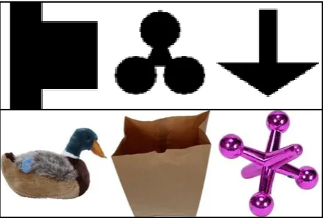
[image:7.595.58.291.420.577.2]In the experiments presented below, we provide a critical test of whether statistical learning in the visual modality leads to the memorization of recurring chunks. Specifically, we extend Endress and Mehler’s (2009b) re-sults to the visual modality using two stimulus sets: the non-sense shapes used by Fiser and Aslin (2002a), and the real-world objects used by Brady, Konkle, Alvarez, and Oliva (2008) (see Figure 2; while our stimuli are visual shapes, we refer to shape triplets as “words” in line with the auditory literature.)
Figure 2. Example objects used in the current experi-ments. Top: objects from Fiser and Aslin (2002a). Bot-tom: objects from Brady et al. (2008)
We explore this issue in the visual modality for two reasons. First, we seek to circumvent the native lan-guage effects that appeared in this literature by using a modality that is plausibly less affected by the partic-ipants’ native language. While visual statistical learn-ing does not seem to correlate with auditory statistical learning (Siegelman & Frost, 2015), the underlying prin-ciples might be similar nonetheless (Frost et al., 2015).
As a result, visual statistical learning is our best guess as to how statistical learning might operate in the auditory domain when people are not affected by prior experience with a language.
Second, given that visual statistical learning does not correlate with auditory statistical learning (Siegelman & Frost, 2015), it is important to find out how statistical learning “works” in the visual modality with respect to memorization.
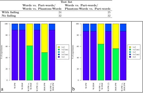
The experiments are summarized in Table 1. To fore-shadow our results, in Experiments 1 and 2, we found that words are preferred to part-words, words are not preferred to phantom-words, and phantom-words are preferred to part-words. However, we also found two results that were unpredicted (albeit with very small effect sizes): phantom-words were preferred to words, and the phantom-word vs. part-words discrimination was easier than the word vs. part-word discrimination.
In Experiment 3 and 4, we asked whether increased exposure would affect the results. However, contrary to expectation, performance did not even improve on the word vs. part-word discrimination, and became numer-ically worse.
In Experiments 5 and 6, participants were familiar-ized with visual streams where “words” were separated by blank screens. In the auditory domain, Endress and Mehler (2009b) showed that additional cues (e.g., from prosody) established a preference for words over phantom-words, and suggested that such cues might help participants memorizing actual items. Here, we found that performance improved, though we also found differences from the equivalent auditory experiments that most likely reflect true modality differences.
T ab le 1 Su m m ary of the c u rr e nt e x p e ri m e nts . In the “ou tc om e ” col um n, W stands for w or ds , PW for p ar t-wor ds (i .e ., low -T P it e ms ), an d PhW fo r phantom -wo rds . T he “g re ate r than ”, “ sma ll e r than ” and “e q u al it y” sig n s st and for the pr e se nc e or ab se nc e of stati sti cal ly si g ni fic an t pr e fe re nc e s or di ffe re nc e s ac cor di ng to the m ai n anal ys e s. F or e x am ple , (W > P W) > (W = Ph W ) m eans that p ar ti c ip ants had a pr e fe re n ce for wor ds ov e r p a rt-w or d s, ha d no si g ni fic ant pr e fe re nc e for w or ds ov e r phant om-w or d s, an d tha t the pr e fe re nc e for w or ds ov e r p ar t-wor ds w as si g ni fic antl y g re ate r than the pr e fe re nc e for wor ds ov e r phantom -wor ds . # Re p et iti on s/ B re ak b et w . E xp . # p art ic ip an ts S ti m ul i a w or d w ord s Ou tcom e b 1a, b 63 F& A, Br ad y 50 n o (W > P W) > (W < P hW ) 2a 20 F & A 50 no (W > P W) = (P hW > P W) 2b ,c 62 F & A, B rad y 50 no (W > P W) = (P hW > P W) 2a, b, c 82 F &A, Br ad y 50 no (W > P W) < (P hW > P W) 3a, b 41 F& A, Br ad y 100 n o (W = PW ) = (W = P hW ) 4 20 F & A 100 no (W = P W) = (P hW = PW ) 5a, b 55 F& A, Br ad y 50 y es (W > P W) > (W > P hW ) 6 13 Br ad y 50 y es (W > P W) < (P hW > P W) aF &A : F iser a n d A sl in (2 0 0 2 a ); B ra d y: B ra d y et a l. (2 0 08 ) bW: W o rd ; P W: P a rt -W o rd ; Ph W : Ph an to m -W o rd
Chunks vs. TPs with visual stimuli
Experiment 1: Are participants sensitive to fre-quency information?
In Experiment 1, participants were familiarized with a sequence of visual stimuli that conformed to the same statistical constraints as in Endress and Mehler’s (2009b) experiments. Following this, they had to choose between words and part-words, and between words and phantom-words.
Materials and methods.
A note on sample sizes and the statistical
ap-proach. As shown in Table 1, the experiments differ
in sample size. These differences arose for “historic” rea-sons. Specifically, in Experiments 1 to 5, we aimed for at least 20 or 30 participants per condition (depending on participant availability), and included the number of participants that could be recruited in a given period of time. Experiments 6 was aborted after a dozen partic-ipants after it became clear that the effects of interest were extremely unlikely to change with larger sample sizes.
For convenience, we will use null-hypothesis signifi-cance testing, despite its well-known drawbacks, includ-ing that some type I and II errors are expected when enough experiments are run. However, data are pre-sented as scatter plots. Readers can thus perform their own intuitive Bayesian analysis by weighing their con-clusion by their prior beliefs in them.
To provide evidencefor null-hypotheses, we will use likelihood ratio analyses inspired by Glover and Dixon (2004). For example, to establish whether a condition differs from the chance level of 50%, we fit two models, assuming that the data is normally distributed. The
alternative model estimates the variance and the mean from the data. In contrast, the null model estimates only the variance from the data, and sets the mean to 50%. As a result, the alternative model has one more parameter than the null model (i.e., the mean). We then use the fitted models to calculate the likelihood of the data, given the model. To account for the different numbers of parameters, we then use the likelihoods to calculate the Akaike Information Criterion (AIC) and the Bayesian Information Criterion (BIC). We use these information criteria as corrected likelihoods to calculate likelihood ratios in favor of or against the null hypothe-sis. Our likelihood ratios are thus really ratios of AIC’s and BIC’s.
Participants. 31 Catalan/Spanish bilinguals (25
partici-pants took part in only one experiment from the current series.
Apparatus. Stimuli were presented on a Philips
109B CRT monitor at a resolution of 1280 ×960 pix-els and a refresh rate of 60 Hz. The experiment was administered in a soundproofed booth and was run us-ing the Matlab psychophysics toolbox (Brainard, 1997; Pelli, 1997).
Materials. The stimuli in Experiment 1a were the
visual shapes used by Fiser and Aslin (2002a); the stim-uli in Experiment 1b were pictures of real-world objects used by Brady et al. (2008). The specific stimuli were randomly selected for each participant.
For the familiarization sequence, visual “words” were constructed such that there would be items that would not appear in the sequences, but that would have ex-actly the same transitional probabilities (TPs) between the first and the second, the second and the third, and the first and the third shape as the words; for mnemonic purposes, we call these items phantom-words.
For constructing the words, we first selected two phantom words, and then chose the actually occurring words accordingly (see Figure 1). For the phantom-word ABC, we included in the stream the three phantom-words ABG, HBC and AJC, where each letter represents a shape. For the phantom-word DEF, the stream con-tained the three words DEG, HEF and DJF. In this way, TPs between adjacent or non-adjacent shapes within words (and phantom-words) were .5, and TPs across word boundaries were .33 on average (range: .28 — .39). The familiarization sequence was created by ran-domly concatenating placeholders for the six words so that the set of images that formed words for an in-dividual participant varied across participants without changing the statistical structure of the familiarization. Each word appeared 50 times in this sequence. This ran-dom sequence was the same for all participants.5 How-ever, the correspondence between placeholders and im-ages was randomized for each participant. Each image was shown for 1 s with no blank between images, lead-ing to a familiarization duration of 15 min. Stimuli were presented on a gray background (RGB code B4B4B4).
The Fiser and Aslin (2002a) stimuli were presented at a size of 136 × 136 pixels (approximately 4.1 cm ×
4.1 cm), subtending a visual angle of 1.96o× 1.96o at a typical viewing distance of 60 cm. The Brady et al. (2008) stimuli were presented at a size of 256×256 pix-els (approximately 7.7 × 7.7 cm), subtending a visual angle of 3.67o×3.67oat a typical viewing distance of 60 cm.
Procedure. Participants were informed that they
would see a sequence of visual shapes. Following this, they saw the stimuli one after the other.
Before the test phase, participants were informed that they would see pairs of sequences of shapes, and that they had to indicate which of these shape sequences was more likely to come from the familiarization sequence. The test triplets were presented one after the other, with a blank screen of 1 s between the triplets.
Pairs of test triplets could be of two types. In the first one, participants had to choose between words and phantom-words. Words and phantom-words could over-lap either in their first and second, their first and third, or their second and their shape; each overlap type was represented equally in the test pairs.
In the remaining trials, participants had to choose between words and part-words. Part-words could be of two types that were equally represented in the test pairs; they could either comprise one shape of the first word and two shapes of the next word (type CAB, if the stream is represented as a shape sequence ABCAB-CABC...), or of two shapes of the first word and one shape of the second word (type BCA). Most part-words shared two shapes with the word they were presented with.
There were 12 Word vs. Phantom-Word test pairs, half with the word presented first, as well as 24 Word vs. Part-Word test pairs, half with the word presented first. In addition to a different random assignment between shapes and placeholders, test pairs were presented in a different random order for each participant, with the constraint of not having more than three trials in a row with the word as the first or the second item, and not having more than three trials in a row with the same type of comparison.
Responses were collected from pre-marked keys on the keyboard.
Results and discussion. As shown in Figure 3,
participants preferred words over part-words signifi-cantly more than expected by chance (M = 58.27%,
SD = 12.75%), t(62) = 5.14, p < .0001, Cohen’s d = .65, CI.95 = 55.05%, 61.48%. A likelihood ratio analy-sis suggested that the alternative hypotheanaly-sis was 70,403 times more likely than the null hypothesis.
As in Endress and Mehler (2009b), participants did not prefer words to phantom-words. Here, however, they preferred words significantlylessthan expected by chance (M = 45.5%,SD = 15.25%),t(62) = 2.34,p = .023, Cohen’s d = .29, CI.95 = 41.66%, 49.34%. How-ever, the likelihood ratio in favor of the alternative hy-pothesis was just 1.95.
This result is unexpected by any account; after all, there is no reason to prefer phantom-words to words.
5The number of repetitions per shape is less than in EM.
0 20 40 60 80 100
Words vs. Phantom−Words and Words vs. Part−Words (Fiser & Aslin and Brady et al. stimuli)
% Choices of w
ords against...
● ● ● ●●●●●●●● ●●●●●● ●●●●● ●●● ●●●●● ●
● ●● ●●●●● ●●●●●●●●●●● ●●●●● ●●●● ●●● ●
● ● ●● ● ●●●●●●● ●●●● ●●●●●● ● ●●●●● ● ●●
● ● ●● ●● ●● ● ●●●●●●● ● ●●●● ●●●● ●● ●●●● ●
...phantom− words
...part− words
Fiser & Aslin Brady et al. Fiser & Aslin Brady et al.
45.2 % 45.8 %
59.4 %
[image:10.595.56.282.91.319.2]57.2 %
Figure 3. Results of Experiment 1. Circles represent individual participants and diamonds sample averages. Participants preferred words to part-words, but failed to prefer words to phantom-words.
Given that the stimuli were randomly selected for each participant, these results cannot be due to a preference for specific phantom-words. As a result, there remain two possibilities. First, these results might reflect a type I error. After all, the effect size of .29 is small, and visual inspection of Figure 3 reveals that the data with just 12 trials is rather discontinuous. In line with this interpre-tation, a multinomial test did not reach significance,p= .0825.6 Alternatively, these results might be due to the single order of placeholders that was used to create the familiarization stream for all participants. Be that as it might, the current results replicate the finding that Italian participants do not prefer words to phantom-words. If the significant preference for phantom-words is due to the specific ordering of the placeholders and not a type I error, they would also show that statistical learning is sensitive to the specific order of items, which might create important problems if it were used in natu-ral language acquisition. We will come back to this issue in the discussion of Experiment 2, where the concern of using only a single randomization of placeholders will be addressed.
To compare the test trial types, we performed an ANOVA with the within-participant predictor Trial Type (word vs. part-word or word vs. phantom-word) and the between-participant predictor Stimulus Set (Fiser and Aslin (2002a) vs. Brady et al. (2008)) as
well as their interaction. The main effect of Trial Type reached significance, F(1,61) = 29.51,p <.0001, η2
p =
.325, suggesting that it was significantly harder to re-ject phantom-words compared to words than part-words compared to words. This result replicates previous find-ings with both Italian and French speakers, and suggests that TP computations do not necessarily lead to the ex-traction of perceptual units. Finally, neither the main effect of Stimulus Set,F(1,61) = .09,p= .77,η2
p= .001, nor the interaction between these factors,F(1,61) = .39,
p = .537,η2
p = .004, reached significance.
7
Experiment 2: Do participants prefer unseen
high-TP items to familiar low-TP items?
Experiment 2 was similar to Experiment 1, except that, during test, participants had to choose between words and part-words, and between phantom-words and part-words.
Materials and methods. As in Experiment 1,
Experiment 2 used the stimuli from Fiser and Aslin (2002a) (Experiment 2b) and Brady et al. (2008) (Ex-periment 2c). In Ex(Ex-periment 2b and 2c, as in Experi-ment 1, the correspondence between image placeholders and images was randomized for each participant.
In Experiment 2a, the stimuli were again those used by Fiser and Aslin (2002a), but they were presented at a faster rate on a smaller screen. (This was not due to a design decision, but rather because Experi-ment 2a was originally a pilot experiExperi-ment.) Crucially, the randomization across participants in Experiment 2a differed from that in Experiments 2b and 2c. Experi-ment 2a comprised two “languages” such that the words and phantom-words in Language 1 were part-words in Language 2 and vice versa. For these reasons, we will analyze Experiment 2a separately. The design of Exper-iment 2a is shown in Table 2.
Participants. 20 Catalan/Spanish bilinguals (17
females, 3 males, mean age 22.4, 19-29) took part in Experiment 2a, 30 Catalan/Spanish bilinguals (19 fe-males, 11 fe-males, mean age 22.5, 19-31) took part in
6In this analysis, we tabulated how many participants
achieved different counts of correct responses, and compared this distribution to a binomial distribution with 12 trials and a success probability of .5, using Pearson’s χ2 to
cal-culate the distance between the expected and actual distri-butions. This difference was estimated in 106 Monte Carlo
trials using the EMTRpackage, version 1.1 (https://cran.r-project.org/web/packages/EMT/).
7We also analyzed word vs. part-word trials in an
Table 2
Design of Experiment 2a
L1 L2
Phantom-words ABC DEF CDE FAB
Words ABG DEG CDJ FAJ
HBC HEF GDE GAB
AJC DJF CHE FHB
Experiment 2b, and 32 Catalan/Spanish bilinguals (21 females, 11 males, mean age 20.8, 18-26) took part in Experiment 2c.
In Experimentr 2b, two additional participants were excluded from analysis. One asked for instructions dur-ing the test phase, and the first few trials were answered by the experimenter, and thus randomly. The second participant was excluded for walking out of the test booth during the experiment or to software crashes, but we did not record which of these two reasons applied to the participant.
Apparatus. Experiment 2a was administered on a
Macbook Pro in a soundproofed booth using Psyscope X (http://psy.ck.sissa.it). The apparatus for Experi-ments 2b and 2c was the same as in Experiment 1.
Materials. In Experiment 2a, each participant
was familiarized with one of two familiarization streams, corresponding to the two languages de-scribed above. Shapes were taken from Fiser and Aslin (2002a). They were concatenated us-ing the catmovie utility from the QTCoffee package (http://www.3am.pair.com/QTCoffee.html). The con-catenation was saved using the H.264 codec and the mov container format with a frame rate of 4 frames/s. Shapes were presented at a rate of 750 ms per shape and had a size of 68×68 pixels. However, using Psyscope, the pre-sentation rate was slowed down to about 1 s per shape (940 ms), and the image size was scaled to 200 × 200 pixels.
The materials for Experiments 2b and 2c were the same as for Experiment 1, except that a different ran-dom ordering of placeholders for words during familiar-ization was used. This ordering was the same for all par-ticipants, but, as in Experiment 1, the correspondence between placeholders and actual images was randomized for each participant.
Procedure. The procedure was identical to that in
Experiment 1, except that participants had to choose between words and part-words (24 trials) and between phantom-words and part-words (8 trials). As in Experi-ment 1, each test item type occurred as the first item on half of the trials. Trials were randomized for each par-ticipant with the same constraint as in Experiment 1.
Results and discussion.
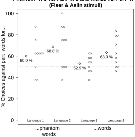
Experiment 2a. As shown in Figure 4,
partici-pants in Experiment 2a preferred words to part-words (M = 58.12%, SD = 12.28%),t(19) = 2.96,p = .008, Cohen’s d = .66, CI.95 = 52.38%, 63.87%. The like-lihood ratio in favor of the alternative hypothesis was 17.9. Participants also preferred phantom-words to part-words (M = 64.38%,SD = 18.26%),t(19) = 3.52,
p = .0023, Cohen’s d = .79, CI.95 = 55.83%, 72.92%. The likelihood ratio in favor of the alternative hypothe-sis was 109.8.
0 20 40 60 80 100
Phantom−W's vs. Part−W's and Words vs. Part−W's (Fiser & Aslin stimuli)
% Choices against par
t−w
ords f
or
...
●● ● ●●●●● ● ●
● ●●● ●●● ●● ●
● ●● ● ●● ●● ●●
● ●● ● ● ● ● ●● ●
...phantom− words
...words
Language 1 Language 2 Language 1 Language 2
60.0 %
68.8 %
52.9 %
63.3 %
Figure 4. Results of Experiment 2a. Circles repre-sent individual participants and diamonds sample av-erages. Participants preferred words to part-words and also phantom-words to part-words.
An ANOVA with Trial Type (word vs. part-word or phantom-word vs. part-word) as within-participant predictor and Language as between-participant predic-tor yielded no main effect of Language,F(1,18) = 2.72,
p = .117,η2
p = .131, nor of Trial Type,F(1,18) = 3.21,
p = .090, η2p = .151, nor an interaction between these factors, F(1,18) = .06, p= .814, η2
p = .003.
Experiments 2b and 2c. As shown in Figure 5,
the performance in word vs. part-word trials was rel-atively poor (M = 53.36%, SD = 11.44%), yet better than expected by chance, t(61) = 2.31, p = .024, Co-hen’s d = .29, CI.95 = 50.46%, 56.26%. However, the likelihood ratio for the non-null hypothesis was just 1.84. In phantom-word vs. part-word trials, participants preferred phantom-words over part-words (M = 57.86%,
[image:11.595.314.539.219.448.2]non-null hypothesis was 8.41.
0 20 40 60 80 100
Phantom−W's vs. Part−W's and Words vs. Part−W's (Fiser & Aslin and Brady et al. stimuli)
% Choices against par
t−w
ords f
or
...
●● ●●● ●●●● ●●●●● ●●●●●●●●● ●● ●●● ●●
● ●●●●●●●● ●●●● ●●●●●●●●● ●●●●● ●●●● ●
● ● ●●● ●● ●●●● ●●●●● ●●●● ●●●●●●●● ● ●
●● ●●●● ●● ●● ●●●● ●●● ●●●●● ●●●●●● ●● ●●
...phantom− words
...words
Fiser & Aslin Brady et al. Fiser & Aslin Brady et al.
55.8 %
59.8 %
54.6 %
[image:12.595.315.538.95.317.2]52.2 %
Figure 5. Results of Experiments 2b and c. Circles represent individual participants and diamonds sample averages. Participants preferred words to part-words and also phantom-words to part-words.
In an ANOVA with the within-participant predic-tor Trial Type (word vs. part-word or phantom-word vs. part-word) and the between-participant predictor Stimulus Set (Fiser and Aslin (2002a) vs. Brady et al. (2008)) as well as their interaction, neither the main ef-fect of Stimulus Set,F(1,60) = .05,p= .824,η2
p <.001, nor the interaction,F(1,60) = 1.45,p= .233,η2
p= .023, reached significance. However, the main effect of Trial Type approached significance,F(1,60) = 2.97,p= .09, η2
p = .046. We will discuss this result below.
Combined analysis. In a combined analysis of
Experiments 2a through 2c, participants preferred words to part-words (M = 54.52%, SD = 11.75%), t(81) = 3.48,p= .0008, Cohen’sd= .38,CI.95= 51.94%, 57.10% (see Figure 6). While the likelihood ratio for the non-null hypothesis was 47.8, performance was still relatively poor.
Participants also preferred phantom-words over part-words (M = 59.45%,SD = 20.75%),t(81) = 4.13,p <
.0001, Cohen’s d = .46, CI.95 = 54.89%, 64.01%. The likelihood ratio in favor of the non-null hypothesis was 547.8
In an ANOVA with the within-participant predictor Trial Type (word vs. part-word or phantom-word vs. part-word) and the between-participant predictor Stim-ulus Set (Experiments 2a and 2b vs. Experiment 2c) as
0 20 40 60 80 100
Phantom−W's vs. Part−W's and Words vs. Part−W's (Combined stimuli)
% Choices against par
t−w
ords f
or
...
●● ●●●● ●●●●●●●●●●●●●●● ●●●●●●●●●●●●● ●●●●●●●●●●●●●●●●●●●●●●● ●●●●●●●●●●●
●●●●●●●●●● ●●●●
●● ● ●●●●●● ●●●●● ●●●●●●● ●●●●●●●●●●● ●●●●●●●●●●● ●●●●●●●●●●●● ●●●●●●●●●●●●●●●●● ●●●
●●● ●●● ●
...phantom− words
...words 59.5 %
54.5 %
Figure 6. Results of Experiment 2a through c. Circles represent individual participants and diamonds sample averages. Participants preferred words to part-words and also phantom-words to part-words.
well as the interaction, neither the main effect of Stim-ulus Set, F(2,79) = 1.30,p = .279, η2
p = .032, nor the interaction, F(2,79) = .9,p = .420,η2
p = .020, reached significance. Surprisingly, however, the main effect of Trial Type reached significance, F(1,79) = 5.28, p = .024,η2
p= .061. According to this result, the preference for phantom-words over part-words was greater than the preference for words over part-words.
To assess the reliability of the surprising effect of Trial Type, we performed a number of follow-up analyses (see Appendix A). These analyses suggest that the effect of Trial Type is small, and carried by a subset of the par-ticipants. However, before dismissing this small effect as a type I error, it should be noted that about a third of participants generally perform around the chance level in typical statistical learning experiments (Frost et al., 2015). The current results thus reveal a small effect that is relatively consistent across experiments, but has no obvious explanation.
Discussion. Experiments 1 and 2 replicate the
crucial results previously obtained with Italian speakers: the word vs. phantom-word discrimination is harder than the word vs. part-word one, phantom-words are
8We did not analyze word vs. part-word trials as a
[image:12.595.56.281.120.342.2]preferred to part-words, and words are not preferred to phantom-words (Endress & Mehler, 2009b).
However, Experiments 1 and 2 also reveal two un-expected results. In Experiment 1, participants signif-icantly prefer phantom-words to words, and in Experi-ment 2, the phantom-word vs. part-word discrimination is easier than the word vs. phantom-word discrimina-tion, although the effect size was rather small in both cases.
There are three possible explanations of these results. First, they might be type I errors. After all, the ef-fect sizes are rather small, and the bootstrap analysis of Experiment 2 (see Appendix A) shows that they are so small that they would probably not be detected in the smaller sample sizes used in typical statistical learn-ing experiments. Further, the effect sizes observed here are somewhat smaller than in comparable earlier exper-iments, perhaps because the differences in TPs between words and part-words were relatively subtle. For ex-ample, Fiser and Aslin (2002a) observed an effect size (Cohen’s d) on the word vs. part-word discrimination with the same material as used here of 1.7 when words were pitted against part-words of typeCAB, and of .4 when words were pitted against part-words of typeBCA (though both effects relied on only 8 participants). How-ever, in the current experiments (that used both CAB andBCApart-words), the effect sizes reached .65 in Ex-periment 1, and .66 in ExEx-periment 2a, and .29 in Experi-ment 2b and c. Performance thus seems to be somewhat worse than in previous studies. However, the fact that the surprising results were relatively systematic across Experiments 1 and 2 makes a type I error somewhat less likely.
Second, in each experiment, only a single random-ization of the sequence of image placeholders was used (while the correspondence between the placeholders and the actual images were randomized for each partici-pant). Possibly, these randomizations made it particu-larly easy to recognize phantom-words even though they never appeared in the familiarization streams, though it is entirely unclear which features of the randomizations might have had such an effect. However, Experiment 1, Experiments 2b and c and Language 1 of Experiment 2a each used different randomizations. As a result, it would be somewhat surprising if each of these randomizations had independently made phantom-words easier to rec-ognize.
Third, the effect might have arisen due the use of test lists with two different trial types (words vs. part-words and part-words vs. phantom-part-words in Experiment 1, and words vs. words and phantom-words vs. part-words in Experiment 2). However, this explanation is rather unlikely as well, and requires additional
as-sumptions.9 Be that is it might, in studies where
French speakers were tested with auditory stimuli, ex-periments with just one test trial type and exex-periments with two test trial types yielded undistinguishable re-sults (Perruchet & Poulin-Charronnat, 2012). Because none of the different possible explanations of these sur-prising results seems particularly convincing, we tenta-tively conclude that they probably represent type I er-rors.
Be that as it might, the crucial results of Experi-ments 1 and 2 are that the word vs. phantom-word discrimination is harder than the word vs. part-word one (with an effect size of η2
p = .325), that phantom-words are preferred to part-phantom-words (with an effect size of Cohen’s d = .46), and that words are not preferred to phantom-words. These results thus support the con-clusions that a sensitivity to TPs does not imply that TPs can be used to store words in memory (Endress & Mehler, 2009b). Further, these results suggest that even relatively weak differences in TPs count more than differences in chunk frequency.
Experiment 3: Are participants sensitive to fre-quency information with twofold exposure?
In Experiments 1 and 2, the participants’ perfor-mance was relatively poor even on word vs. part-words trials. In Experiments 3 and 4, we attempted to improve performance by playing the familiarization streams twice. In Experiment 3, participants were tested on word vs. part-words trials and word vs. phantom-word trials. In Experiment 4, they were tested on word vs. part-words trials and phantom-word vs. part-word trials.
Materials and methods. Experiment 3 was
iden-tical to Experiment 1, except that the familiarization stream was played twice, resulting in 100 repetitions per word. The stimuli in Experiments 3a and 3b were taken
9For example, if we assume that, in Experiment 1, the
from Fiser and Aslin (2002a) and Brady et al. (2008), respectively.
21 Catalan/Spanish bilinguals (14 females, 7 males, mean age 22.0, 17-35) took part in Experiment 3a. 20 Catalan/Spanish bilinguals (14 females, 6 males, mean age 19.9, 18-26) took part in Experiment 3b.
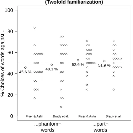
Results and discussion. As shown in Figure 7,
participants showed no preference for words over part-words (M = 52.24%,SD = 11.3%), t(40) = 1.27,p = .213, Cohen’sd = .2,CI.95 = 48.67%, 55.8%. The like-lihood ratio in favor of the null hypothesis was 2.87.
0 20 40 60 80 100
Words vs. Phantom−Words and Words vs. Part−Words (Twofold familiarization)
% Choices of w
ords against...
● ●●● ●● ●●●●● ●●● ●●●●● ● ●
● ●● ● ●● ●● ●● ●●●● ●●●● ●●
● ● ● ● ● ●●●●● ●● ●●● ●●● ●● ●
● ● ● ●●●●● ● ●●●●● ●● ● ●● ●
...phantom− words
...part− words
Fiser & Aslin Brady et al. Fiser & Aslin Brady et al.
45.6 % 48.3 %
[image:14.595.56.281.240.464.2]52.6 % 51.9 %
Figure 7. Results of Experiment 3. Circles represent individual participants and diamonds sample averages. Compared to Experiment 1, the exposure to the famil-iarization stream was doubled.
Participants showed no preference for words over phantom-words either (M = 46.95%, SD = 18.14%),
t(40) = 1.08,p= .288, Cohen’sd= .17,CI.95= 41.23%, 52.68%. The likelihood ratio in favor of the null hypoth-esis was 3.59. An ANOVA with the within-participant predictor Trial Type (word vs. part-word or word vs. phantom-word) and the between-participant predictor Stimulus Set (Fiser and Aslin (2002a) vs. Brady et al. (2008)) as well as their interaction yielded neither a main effect of Trial Type, F(1,39) = 2.61, p = .114, η2
p = .0623, nor of Stimulus Set, F(1,39) = .08, p = .776,η2
p= .002, nor an interaction between these factors,
F(1,39) = .27,p= .606,η2
p = .006.10
Comparing Experiment 1 and 3, an ANOVA with the within-participant predictor Trial Type (word vs. part-word or part-word vs. phantom-word) and the
between-participant predictors Stimulus Set (Fiser and Aslin (2002a) vs. Brady et al. (2008)) and Familiarization Duration (50 vs. 100 repetitions per word) as well as all interactions yielded only a main effect of Trial Type, F(1,100) = 26.15, p < .0001, η2
p = .2, and a marginal Familiarization Duration by Trial Type inter-action,F(1,100) = 3.63,p= .060,η2
p= .028. A two-fold familiarization therefore failed to strengthen statistical computations over visual stimuli.
Experiment 4: Do participants prefer unseen
high-TP items to familiar low-TP items with twofold exposure?
Materials and method. Experiment 4 was
identi-cal to Experiment 2a, with three exceptions. First, and crucially, the familiarization stream was played twice, yielding 100 repetitions per word. Second, shapes were presented at a rate of about 716 ms per shape (as op-posed to 1 s/shape), and had a size of 68×68 pixels (as opposed to 136×136 pixels). This was not a design de-cision based on the results of Experiments 1 and 2 but rather a consequence of the fact that this experiment was an initial pilot experiment.
20 Catalan/Spanish bilinguals (11 females, 9 males, mean age 24.6, 18-44) took part in Experiment 4. Two additional participants were excluded from analysis. One walked out of the test booth to ask for instruc-tions during the familiarization, and missed at least one minute of the familiarization stream. For the other par-ticipant, the computer crashed before reaching the test phase.
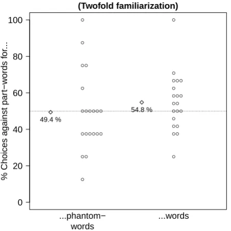
Results. As shown in Figure 8, participants had
no preference for words over part-words (M = 54.79%,
SD = 15.9%),t(19) = 1.35,p = .193, Cohen’sd = .3, CI.95= 47.35%, 62.23%. The likelihood ratio in favor of the null hypothesis was 1.80. Participants had no pref-erence for phantom-words over part-words either (M = 49.38%,SD = 21.64%), t(19) = .13,p= .899, Cohen’s
d = .029, CI.95 = 39.25%, 59.5%. The likelihood ratio in favor of the null hypothesis was 4.43.
An ANOVA with the within-participant factor Trial Type (word vs. part-word or word vs. phantom-word) and the between-participant factor Language yielded no main effect of Trial Type, F(1,18) = 2.24, p = .152, η2
p = .11, nor of Language, F(1,18) = .01, p = .918, η2
p = .0006, nor an interaction,F(1,18) = .01, p= .91,
10We also analyzed word vs. part-word trials in an
0 20 40 60 80 100
Phantom−W's vs. Part−W's and Words vs. Part−W's (Twofold familiarization)
% Choices against par
t−w
ords f
or
...
● ● ● ● ● ● ● ● ● ● ● ● ● ● ● ● ● ● ● ●
● ● ● ● ● ● ● ● ● ● ● ● ● ● ● ● ● ● ● ●
...phantom− words
...words 49.4 %
[image:15.595.56.282.91.317.2]54.8 %
Figure 8. Results of Experiment 4. Circles represent individual participants and diamonds sample averages. Compared to Experiment 2, the exposure to the famil-iarization stream was doubled.
η2
p = .0007.11
Comparing Experiments 2a and 4, an ANOVA with the within-participant factor Trial Type (word vs. part-word or part-word vs. phantom-word) and the between-participant factors Language and Familiarization Dura-tion yielded a significant Test Type by FamiliarizaDura-tion Duration interaction, F(1,36) = 5.38, p = .026, η2
p =
.13, as well as a marginal main effect of Familiarization Duration,F(1,36) = 3.47,p = .071,η2
p = .084.
Discussion. The results of Experiment 4 are
unex-pected. While increasing the exposure improved sensi-tivity to statistical cues in other experiments (e.g., En-dress & Bonatti, 2007; Pe˜na, Bonatti, Nespor, & Mehler, 2002), doubling the familiarization duration in Exper-iment 4 worsened participants’ performance consider-ably. There is no immediate explanation for these re-sults, except that the TP differences between words and part-words were relatively subtle in the current exper-iments. As a result, participants might learn the asso-ciations so well that they can longer discriminate items on the basis of the strength of TPs if they have been fa-miliarized for too long with these items. Alternatively, and as discussed in the General Discussion, statistical computations might not be as robust as they are often believed to be.
Experiment 5: Are participants sensitive to fre-quency information after segmented familiariza-tions?
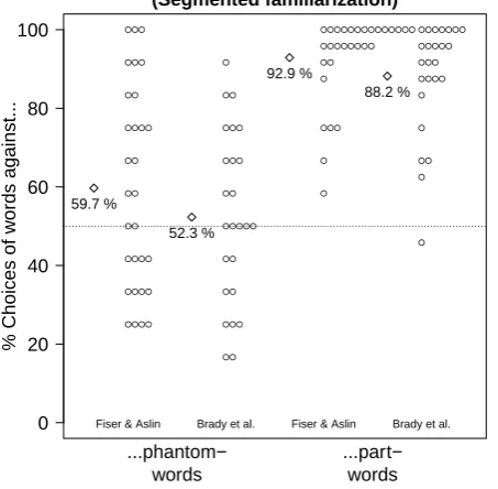
In the auditory modality, (Italian) participants pre-ferred words to phantom-words when the familiarization streams contained explicit segmentation marks, such as short silences between words or lengthened word-final syllables (Endress & Mehler, 2009b). Endress and Mehler (2009b) concluded that such additional cues (that might be provided by prosody in real speech) help learners memorize actual items. In Experiments 5 and 6, we ask whether these results transfer to the visual modality. We thus assess whether the word vs. phantom-word discrimination would improve when words are separated by blank screens during familiariza-tion.
Materials and methods. Experiment 5 was
iden-tical to Experiment 1, except that words in the familiar-ization stream were separated by a blank screen of 1 s. The stimuli in Experiment 5a were taken from Fiser and Aslin (2002a), and those in Experiment 5b from Brady et al. (2008).
30 Catalan/Spanish bilinguals (19 females, 11 males, mean age 20.7, 17-23) took part in Experiment 5a. 25 Catalan/Spanish bilinguals (20 females, 5 males, mean age 20.3, 18-25) took part in Experiment 5b.
Results. As shown in Figure 9, participants
pre-ferred words over part-words (M = 90.76%, SD = 12.8%), t(54) = 23.62, p < .0001, Cohen’s d = 3.2, CI.95 = 87.3%, 94.22%. The likelihood ratio in favor of the alternative hypothesis was 1.88×10120. They also had a marginal preference for words over phantom-words (M = 56.36%,SD = 24.11%),t(54) = 1.96,p = .055, Cohen’s d = .26, CI.95 = 49.85%, 62.88%. How-ever, the likelihood ratio in favor of the null hypothesis was 1.09.
An ANOVA with the within-participant predictor Trial Type (word vs. part-word or word vs. phantom-word) and the between-participant predictor Stimulus Set (Fiser and Aslin (2002a) vs. Brady et al. (2008)) as well as their interaction yielded a main effect of Test Type,F(1,53) = 109.2,p<.0001,η2
p = .673, but not of Stimulus Set, F(1,53) =2.28, p = .137, η2
p = .041, nor an interaction,F(1,53) = .159,p = .691,η2
p = .001.12
11We did not analyze word vs. part-word trials as a
func-tion of the part-word type because we did not record the part-word types.
12We also analyzed word vs. part-word trials in an
0 20 40 60 80 100
Words vs. Phantom−Words and Words vs. Part−Words (Segmented familiarization)
% Choices of w
ords against...
●●●● ●●●● ●●●● ●● ●● ●● ●●●● ●● ●●● ●●●
●● ●●● ●● ●● ●●●●● ●● ●●● ●●● ●● ●
● ● ●●● ● ●● ●●●●●●●● ●●●●●●●●●●●●●●
● ● ●● ● ● ●●●● ●●● ●●●●● ●●●●●●●
...phantom− words
...part− words
Fiser & Aslin Brady et al. Fiser & Aslin Brady et al.
59.7 %
52.3 %
92.9 %
[image:16.595.56.283.97.319.2]88.2 %
Figure 9. Results of Experiment 5. Circles represent individual participants and diamonds sample averages. In contrast to Experiment 1, the familiarization stream contained blank screens of 1 s after each word.
Comparing Experiment 1 and 5, an ANOVA with the within-participant predictor Trial Type (word vs. part-word or part-word vs. phantom-word) and the between-participant predictors Stimulus Set (Fiser and Aslin (2002a) vs. Brady et al. (2008)) and Familiarization Type (continuous vs. segmented) as well as all inter-actions yielded main effects of Test Type, F(1,114) = 133, p < .0001, η2
p = .48, and Familiarization Type,
F(1,114) = 84.56, p <.0001, η2p = .419, as well as an interaction between these factors,F(1,114) = 29.66,p<
.0001, η2
p = .107. Crucially, however, performance im-proved between Experiments 1 and 5 both for word vs. part-word tests,F(1,114) = 191,p <.0001,η2
p= 0.621, and for word vs. phantom-word tests, F(1,114) = 8.8,
p = 0.004,η2
p= 0.07.
Discussion. In the familiarization streams of
Ex-periment 5, words were separated from one another by blank screens of 1 s. Compared to a continuous familiar-ization, these segmentation cues boosted performance in the word vs. part-word trials. In contrast, the prefer-ence for words over phantom-words was significantly im-proved as well, although it remained marginal (though visual inspection of Figure 9 revealed that the poor per-formance was driven by the condition with the Brady et al. (2008) stimuli).
These results are consistent with those of Endress and Mehler’s (2009b) Experiments 3 and 4 in that including
explicit segmentation cues led to a preference for words over phantom-words. However, they differ from these results in that performance on word vs. part-word tri-als improved much more than performance on word vs. phantom-word trials. In Endress and Mehler’s (2009b) experiments, the improvement was similar in both trial types. However, visual inspection of Figure 9 suggests that those participants exposed to the stimulus set taken from Fiser and Aslin (2002a) performed rather similarly to Italian participants in Endress and Mehler (2009b) Experiments 3 and 4.
To the extent that the pattern of results in Exper-iment 5 is different from that in Endress and Mehler’s (2009b) Experiments 3 and 4, the difference probably re-flects a true modality difference. Specifically, in both the auditory and the visual modality in humans (Endress & Bonatti, 2007; Endress & Mehler, 2009a; Endress & Wood, 2011), and in non-human primates (Endress, Carden, Versace, & Hauser, 2010), a familiarization with streams containing explicit segmentation cues can lead participants to accept items that have onsets and offsets that have occurred in these positions during familiar-ization, even if the test item has not been encountered during familiarization. Given that phantom-words have correct onsets and offsets, they might be relatively hard to reject for this reason after a segmented familiariza-tion.
Crucially, at least in the auditory modality, hu-mans readily prefer actual words to items like phantom-words that have only correct edge syllables (see Endress and Bonatti’s (2007) Experiment 8 and Endress and Mehler’s (2009b) Experiments 3 and 4). To the extent that the results of Experiment 5 differ from Endress and Mehler’s (2009b), differentiating actual items from gen-eralizations might be comparatively harder in the visual modality, either due to genuine modality differences, or because the presentation rate is about four times faster in auditory statistical learning experiment. Crucially, however, as in Endress and Mehler’s (2009b) experi-ments, including explicit segmentation cues improved performance on word vs. phantom-word trials as well.
Experiment 6: Do participants prefer unseen
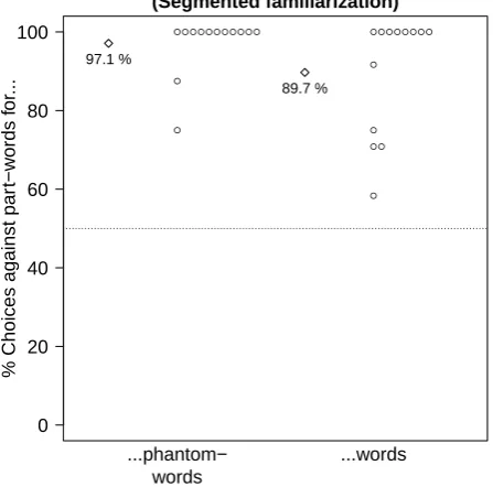
high-TP items to familiar low-TP items with seg-mented familiarizations?
In Experiment 6, the familiarization stream contained blank screens between words, as in Experiment 5. How-ever, in contrast to Experiment 5, participants had to choose between words and part-words, and between phantom-words and part-words.