MATHEMATICIANS
CATHERINE F. HIGHAM∗ AND DESMOND J. HIGHAM†
Abstract. Multilayered artificial neural networks are becoming a pervasive tool in a host of application fields. At the heart of this deep learning revolution are familiar concepts from applied and computational mathematics; notably, in calculus, approximation theory, optimization and linear algebra. This article provides a very brief introduction to the basic ideas that underlie deep learning from an applied mathematics perspective. Our target audience includes postgraduate and final year undergraduate students in mathematics who are keen to learn about the area. The article may also be useful for instructors in mathematics who wish to enliven their classes with references to the application of deep learning techniques. We focus on three fundamental questions: what is a deep neural network? how is a network trained? what is the stochastic gradient method? We illustrate the ideas with a short MATLAB code that sets up and trains a network. We also show the use of state-of-the art software on a large scale image classification problem. We finish with references to the current literature.
Key words. back propagation, chain rule, convolution, image classification, neural network, overfitting, sigmoid, stochastic gradient method, supervised learning
AMS subject classifications. 68T05, 65K10, 65D15
1. Motivation. Most of us have come across the phrase deep learning. It relates to a set of tools that have become extremely popular in a vast range of application fields, from image recognition, speech recognition and natural language processing to targeted advertising and drug discovery. The field has grown to the extent where sophisticated software packages are available in the public domain, many produced by high-profile technology companies. Chip manufacturers are also customizing their graphics processing units (GPUs) for kernels at the heart of deep learning.
Whether or not its current level of attention is fully justified, deep learning is clearly a topic of interest to employers, and therefore to our students. Although there are many useful resources available, we feel that there is a niche for a brief treatment aimed at mathematical scientists. For a mathematics student, gaining some familiarity with deep learning can enhance employment prospects. For mathematics educators, slipping “Applications to Deep Learning” into the syllabus of a class on calculus, approximation theory, optimization, linear algebra, or scientific computing is a great way to attract students and maintain their interest in core topics. The area is also ripe for independent project study.
There is no novel material in this article, and many topics are glossed over or omitted. Our aim is to present some key ideas as clearly as possible while avoiding non-essential detail. The treatment is aimed at readers with a background in math-ematics who have completed a course in linear algebra and are familiar with partial differentiation. Some experience of scientific computing is also desirable.
To keep the material concrete, we list and walk through a short MATLAB code that illustrates the main algorithmic steps in setting up, training and applying an
∗School of Computing Science, University of Glasgow, UK (
[email protected]). This author was supported by the EPSRC UK Quantum Technology Programme under grant EP/M01326X/1.
†Department of Mathematics and Statistics, University of Strathclyde, UK ([email protected]). This author was supported by EPSRC/RCUK Established Ca-reer Fellowship EP/M00158X/1 and by EPSRC Programme Grant EP/P020720/1.
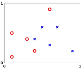
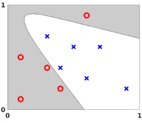
Fig. 2.1.Labeled data points inR2. Circles denote points in category A. Crosses denote points
in category B.
artificial neural network. We also demonstrate the high-level use of state-of-the-art software on a larger scale problem.
Section 2 introduces some key ideas by creating and training an artificial neural network using a simple example. Section 3 sets up some useful notation and defines a general network. Training a network, which involves the solution of an optimization problem, is the main computational challenge in this field. In Section 4 we describe the stochastic gradient method, a variation of a traditional optimization technique that is designed to cope with very large scale sets of training data. Section 5 explains how the partial derivatives needed for the stochastic gradient method can be computed efficiently using back propagation. First-principles MATLAB code that illustrates these ideas is provided in section 6. A larger scale problem is treated in section 7. Here we make use of existing software. Rather than repeatedly acknowledge work throughout the text, we have chosen to place the bulk of our citations in Section 8, where pointers to the large and growing literature are given. In that section we also raise issues that were not mentioned elsewhere, and highlight some current hot topics.
2. Example of an Artificial Neural Network. This article takes a data fitting view of artificial neural networks. To be concrete, consider the set of points shown in Figure 2.1. This showslabeled data—some points are in category A, indicated by circles, and the rest are in category B, indicated by crosses. For example, the data may show oil drilling sites on a map, where category A denotes a successful outcome. Can we use this data to categorize a newly proposed drilling site? Our job is to construct a mapping that takes any point inR2 and returns either a circle or a cross.
Of course, there are many reasonable ways to construct such a mapping. The artificial neural network approach uses repeated application of a simple, nonlinear function.
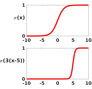
We will base our network on the sigmoid function
σ(x) = 1
1 +e−x, (2.1)
which is illustrated in the upper half of Figure 2.2 over the interval−10≤x≤10. We may regardσ(x) as a smoothed version of a step function, which itself mimics the behavior of a neuron in the brain—firing (giving output equal to one) if the input is large enough, and remaining inactive (giving output equal to zero) otherwise. The sigmoid also has the convenient property that its derivative takes the simple form
Fig. 2.2.Upper: sigmoid function (2.1). Lower: sigmoid with shifted and scaled input.
which is straightforward to verify. Other types of nonlinearity are discussed in Section 8.
The steepness and location of the transition in the sigmoid function may be altered by scaling and shifting the argument or, in the language of neural networks, byweighting andbiasing the input. The lower plot in Figure 2.2 shows σ(3(x−5)). The factor 3 has sharpened the changeover and the shift −5 has altered its location. To keep our notation managable, we need to interpret the sigmoid function in a vectorized sense. For z ∈ Rm, σ :
Rm → Rm is defined by applying the sigmoid
function in the obvious componentwise manner, so that
(σ(z))i=σ(zi).
With this notation, we can set up layers of neurons. In each layer, every neuron outputs a single real number, which is passed to every neuron in the next layer. At the next layer, each neuron forms its own weighted combination of these values, adds its own bias, and applies the sigmoid function. Introducing some mathematics, if the real numbers produced by the neurons in one layer are collected into a vector,a, then the vector of outputs from the next layer has the form
σ(W a+b). (2.3)
Here, W is matrix and b is a vector. We say that W contains the weights and b contains the biases. The number of columns inW matches the number of neurons that produced the vectoraat the previous layer. The number of rows inW matches the number of neurons at the current layer. The number of components in b also matches the number of neurons at the current layer. To emphasize the role of theith neuron in (2.3), we could pick out theith component as
σ
X
j
wijaj+bi
Layer 1 (Input layer)
Layer 2
Layer 3
[image:4.612.175.342.95.198.2]Layer 4 (Output layer)
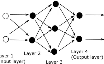
Fig. 2.3.A network with four layers.
where the sum runs over all entries ina. Throughout this article, we will be switching between the vectorized and componentwise viewpoints to strike a balance between clarity and brevity.
In the next section, we introduce a full set of notation that allows us to define a general network. Before reaching that stage, we will give a specific example. Figure 2.3 represents an artificial neural network with four layers. We will apply this form of network to the problem defined by Figure 2.1. For the network in Figure 2.3 the first (input) layer is represented by two circles. This is because our input data points have two components. The second layer has two solid circles, indicating that two neurons are being employed. The arrows from layer one to layer two indicate that both components of the input data are made available to the two neurons in layer two. Since the input data has the formx∈R2, the weights and biases for layer two
may be represented by a matrixW[2]∈
R2×2and a vectorb[2]∈R2, respectively. The
output from layer two then has the form
σ(W[2]x+b[2])∈R2.
Layer three has three neurons, each receiving input inR2. So the weights and biases
for layer three may be represented by a matrix W[3] ∈
R3×2 and a vector b[3] ∈R3,
respectively. The output from layer three then has the form
σW[3]σ(W[2]x+b[2]) +b[3]∈R3.
The fourth (output) layer has two neurons, each receiving input inR3. So the weights
and biases for this layer may be represented by a matrix W[4] ∈R2×3 and a vector
b[4] ∈ R[2], respectively. The output from layer four, and hence from the overall
network, has the form
F(x) =σW[4]σW[3]σ(W[2]x+b[2]) +b[3]+b[4]∈R2. (2.4)
The expression (2.4) defines a functionF:R2→R2in terms of its 23 parameters—
the entries in the weight matrices and bias vectors. Recall that our aim is to produce a classifier based on the data in Figure 2.1. We do this by optimizing over the pa-rameters. We will require F(x) to be close to [1,0]T for data points in category A
and close to [0,1]T for data points in category B. Then, given a new pointx∈ R2, it
would be reasonable to classify it according to the largest component ofF(x); that is, category A ifF1(x)> F2(x) and category B ifF1(x)< F2(x), with some rule to break
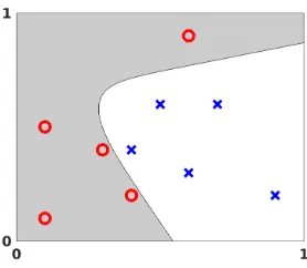
Fig. 2.4. Visualization of output from an artificial neural network applied to the data in Figure 2.1.
ten data points in Figure 2.1 by{x{i}}10
i=1, we usey(x{i}) for the target output; that
is,
y(x{i}) =
1 0
if x{i} is in category A,
0 1
if x{i} is in category B.
(2.5)
Our cost function then takes the form
CostW[2], W[3], W[4], b[2], b[3], b[4]= 1 10
10 X
i=1 1 2ky(x
{i})−F(x{i})k2
2. (2.6)
Here, the factor 1
2 is included for convenience; it simplifies matters when we start
differentiating. We emphasize that Cost is a function of the weights and biases—the data points are fixed. The form in (2.6), where discrepancy is measured by averaging the squared Euclidean norm over the data points, is often refered to as a quadratic cost function. In the language of optimization, Cost is ourobjective function.
Choosing the weights and biases in a way that minimizes the cost function is refered to as training the network. We note that, in principle, rescaling an objective function does not change an optimization problem. We should arrive at the same minimizer if we change Cost to, for example, 100 Cost or Cost/30. So the factors 1/10 and 1/2 in (2.6) should have no effect on the outcome.
For the data in Figure 2.1, we used the MATLAB optimization toolbox to mini-mize the cost function (2.6) over the 23 parameters definingW[2],W[3],W[4],b[2],b[3]
and b[4]. More precisely, we used the nonlinear least-squares solverlsqnonlin. For the trained network, Figure 2.4 shows the boundary where F1(x)> F2(x). So, with
[image:5.612.187.326.100.221.2]this approach, any point in the shaded region would be assigned to category A and any point in the unshaded region to category B.
Figure 2.5 shows how the network responds to additional training data. Here we added one further category B point, indicated by the extra cross at (0.3,0.7), and re-ran the optimization routine.
Fig. 2.5.Repeat of the experiment in Figure 2.4 with an additional data point.
exhaustively search over a 23 dimensional parameter space, and we cannot guarantee to find the global minimum of a non-convex function. Indeed, some experimentation with the location of the data points in Figure 2.4 and with the choice of initial guess for the weights and biases makes it clear that lsqnonlin, with its default settings, cannot always find an acceptable solution. This motivates the material in sections 4 and 5, where we focus on the optimization problem.
3. The General Set-up. The four layer example in section 2 introduced the idea of neurons, represented by the sigmoid function, acting in layers. At a general layer, each neuron receives the same input—one real value from every neuron at the previous layer—and produces one real value, which is passed to every neuron at the next layer. There are two exceptional layers. At the input layer, there is no “previous layer” and each neuron receives the input vector. At the output layer, there is no “next layer” and these neurons provide the overall output. The layers in between these two are called hidden layers. There is no special meaning to this phrase; it simply indicates that these neurons are performing intermediate calculations. Deep learning is a loosely-defined term which implies that many hidden layers are being used.
We now spell out the general form of the notation from section 2. We suppose that the network hasLlayers, with layers 1 andLbeing the input and output layers, respectively. Suppose that layerl, forl= 1,2,3, . . . , L, containsnlneurons. So n1is
the dimension of the input data. Overall, the network maps from Rn1 to
RnL. We
useW[l]∈
Rnl×nl−1 to denote the matrix of weights at layerl. More precisely,w[l]
jkis
the weight that neuronjat layerlapplies to the output from neuronkat layerl−1. Similarly, b[l]∈
Rnl is the vector of biases for layerl, so neuronj at layerl uses the
biasb[jl].
In Fig 3.1 we give an example withL= 5 layers. Here, n1= 4,n2 = 3,n3 = 4,
n4 = 5 and n5 = 2, so W[2] ∈ R3×4, W[3] ∈ R4×3, W[4] ∈ R5×4, W[5] ∈ R2×5,
b[2]∈
R3,b[3]∈R4, b[4]∈R5 andb[5]∈R2.
Given an inputx∈Rn1, we may then neatly summarize the action of the network
by lettinga[jl] denote the output, oractivation, from neuronj at layer l. So, we have
a[1]=x∈Rn1, (3.1)
a[l]=σW[l]a[l−1]+b[l]∈Rnl, forl= 2,3, . . . , L. (3.2)
Layer 1 (Input layer)
Layer 2
Layer 3
Layer 5 (Output layer) W43[3]
[image:7.612.150.367.109.300.2]Layer 4
Fig. 3.1.A network with five layers. The edge corresponding to the weightw[3]43 is highlighted. The output from neuron number 3 at layer 2 is weighted by the factorw43[3]when it is fed into neuron number 4 at layer 3.
forward through the network in order to produce an output a[L] ∈
RnL. At the end
of section 5 this algorithm appears within a pseudocode description of an approach for training a network.
Now suppose we haveN pieces of data, ortraining points, inRn1, {x{i}}N
i=1, for
which there are given target outputs {y(x{i})}N
i=1 in RnL. Generalizing (2.6), the
quadratic cost function that we wish to minimize has the form
Cost = 1 N
N X
i=1 1 2ky(x
{i})−a[L](x{i})k2
2, (3.3)
where, to keep notation under control, we have not explicitly indicated that Cost is a function of all the weights and biases.
4. Stochastic Gradient. We saw in the previous two sections that training a network corresponds to choosing the parameters, that is, the weights and biases, that minimize the cost function. The weights and biases take the form of matrices and vectors, but at this stage it is convenient to imagine them stored as a single vector that we callp. The example in Figure 2.3 has a total of 23 weights and biases. So, in that case,p∈R23. Generally, we will supposep∈Rs, and write the cost function in
(3.3) as Cost(p) to emphasize its dependence on the parameters. So Cost :Rs→R.
We now introduce a classical method in optimization that is often refered to as steepest descent or gradient descent. The method proceeds iteratively, computing a sequence of vectors in Rs with the aim of converging to a vector that minimizes
the cost function. Suppose that our current vector is p. How should we choose a perturbation, ∆p, so that the next vector,p+ ∆p, represents an improvement? If ∆p is small, then ignoring terms of orderk∆pk2, a Taylor series expansion gives
Cost(p+ ∆p)≈Cost(p) +
s X
r=1
∂Cost(p) ∂ pr
Here∂Cost(p)/∂ prdenotes the partial derivative of the cost function with respect to
therth parameter. For convenience, we will let ∇Cost(p)∈Rs denote the vector of
partial derivatives, known as thegradient, so that
(∇Cost(p))r=∂Cost(p) ∂ pr
.
Then (4.1) becomes
Cost(p+ ∆p)≈Cost(p) +∇Cost(p)T∆p. (4.2)
Our aim is to reduce the value of the cost function. The relation (4.2) motivates the idea of choosing ∆pto make∇Cost(p)T∆pas negative as possible. We can address
this problem via the Cauchy–Schwarz inequality, which states that for anyf, g∈Rs,
we have|fTg| ≤ kfk
2kgk2. So the most negative thatfTg can be is−kfk2kgk2,
which happens when f = −g. Hence, based on (4.2), we should choose ∆p to lie in the direction−∇Cost(p). Keeping in mind that (4.2) is an approximation that is relevant only for small ∆p, we will limit ourselves to a small step in that direction. This leads to the update
p→p−η∇Cost(p). (4.3)
Here η is small stepsize that, in this context, is known as the learning rate. This equation defines the steepest descent method. We choose an initial vector and iterate with (4.3) until some stopping criterion has been met, or until the number of iterations has exceeded the computational budget.
Our cost function (3.3) involves a sum of individual terms that runs over the training data. It follows that the partial derivative∇Cost(p) is a sum over the training data of individual partial derivatives. More precisely, let
Cx{i}= 12ky(x{i})−a[L](x{i})k22. (4.4)
Then, from (3.3),
∇Cost(p) = 1 N
N X
i=1
∇Cx{i}(p). (4.5)
When we have a large number of parameters and a large number of training points, computing the gradient vector (4.5) at every iteration of the steepest descent method (4.3) can be prohibitively expensive. A much cheaper alternative is to replace the mean of the individual gradients over all training points by the gradient at a single, randomly chosen, training point. This leads to the simplest form of what is called the stochastic gradient method. A single step may be summarized as
1. Choose an integeriuniformly at random from{1,2,3, . . . , N}. 2. Update
p→p−η∇Cx{i}(p). (4.6)
update (4.6) is not guaranteed to reduce the overall cost function—we have traded the mean for a single sample. Hence, although the phrasestochastic gradient descent is widely used, we prefer to use stochastic gradient.
The version of the stochastic gradient method that we introduced in (4.6) is the simplest from a large range of possibilities. In particular, the index i in (4.6) was chosen by samplingwith replacement—after using a training point, it is returned to the training set and is just as likely as any other point to be chosen at the next step. An alternative is to sample without replacement; that is, to cycle through each of the N training points in a random order. PerformingN steps in this manner, refered to as completing anepoch, may be summarized as follows:
1. Shuffle the integers{1,2,3, . . . , N}into a new order,{k1, k2, k3, . . . , kN}.
2. fori= 1 uptoN, update
p→p−η∇Cx{ki}(p). (4.7)
If we regard the stochastic gradient method as approximating the mean over all training points in (4.5) by a single sample, then it is natural to consider a compromise where we use a small sample average. For some m N we could take steps of the following form.
1. Choosemintegers,k1, k2, . . . , km, uniformly at random from{1,2,3, . . . , N}.
2. Update
p→p−η 1 m
m X
i=1
∇Cx{ki}(p). (4.8)
In this iteration, the set {x{ki}}n
i=1 is known as a mini-batch. There is a without
replacement alternative where, assuming N =Kmfor some K, we split the training set randomly intoKdistinct mini-batches and cycle through them.
Because the stochastic gradient method is usually implemented within the context of a very large scale computation, algorithmic choices such as mini-batch size and the form of randomization are often driven by the requirements of high performance computing architectures. Also, it is, of course, possible to vary these choices, along with others, such as the learning rate, dynamically as the training progresses in an attempt to accelerate convergence. Indeed, an effective algorithm for specifying the learning rate is a key ingredient for practical computations.
Section 6 gives a simple MATLAB code that uses a vanilla stochastic gradient method. In section 7 we describe a state-of-the-art implementation and section 8 has pointers to the current literature.
5. Back Propagation. We are now in a position to apply the stochastic gra-dient method in order to train an artificial neural network. So we switch from the general vector of parameters,p, used in section 4 to the entries in the weight matrices and bias vectors. Our task is to compute partial derivatives of the cost function with respect to each w[jkl] and b[jl]. We saw that the idea behind the stochastic gradient method is to exploit the structure of the cost function: because (3.3) is a linear com-bination of individual terms that runs over the training data the same is true of its partial derivatives. We therefore focus our attention on computing those individual partial derivatives.
Hence, for a fixed training point we regard Cx{i} in (4.4) as a function of the
weights and biases. So we may drop the dependence onx{i} and simply write
C= 12ky−a[L]k2
We recall from (3.2) that a[L] is the output from the artificial neural network. The
dependence ofC on the weights and biases arises only througha[L].
To derive worthwhile expressions for the partial derivatives, it is useful to intro-duce two further sets of variables. First we let
z[l]=W[l]a[l−1]+b[l]∈Rnl, forl= 2,3, . . . , L. (5.2)
We refer toz[jl] as theweighted inputfor neuronjat layerl. The fundamental relation (3.2) that propagates information through the network may then be written
a[l] =σz[l], forl= 2,3, . . . , L. (5.3)
Second, we letδ[l]∈
Rnl be defined by
δ[jl]= ∂ C ∂ z[jl]
, for 1≤j ≤nl and 2≤l≤L. (5.4)
This expression, which is often called the error in the jth neuron at layer l, is an intermediate quantity that is useful both for analysis and computation. However, we point out that this useage of the term error is somewhat ambiguous. At a general, hidden layer, it is not clear how much to “blame” each neuron for discrepancies in the final output. Also, at the output layer,L, the expression (5.4) does not quantify those discrepancies directly. The idea of refering toδ[jl] in (5.4) as an error seems to have arisen because the cost function can only be at a minimum if all partial derivatives are zero, soδj[l] = 0 is a useful goal. As we mention later in this section, it may be more helpful to keep in mind thatδj[l] measures the sensitivity of the cost function to the weighted input for neuronj at layerl.
At this stage we also need to define the Hadamard, or componentwise, product of two vectors. If x, y∈Rn, thenx◦y∈Rn is defined by (x◦y)i =xiyi. In words,
the Hadamard product is formed by pairwise multiplication of the corresponding components.
With this notation, the following results are a consequence of the chain rule.
Lemma 5.1. We have
δ[L] =σ0(z[L])◦(aL−y), (5.5)
δ[l] =σ0(z[l])◦(W[l+1])Tδ[l+1], for 2≤l≤L−1, (5.6) ∂ C
∂ b[jl]
=δj[l], for 2≤l≤L, (5.7)
∂ C ∂ w[jkl]
=δj[l]ak[l−1]. for 2≤l≤L. (5.8)
Proof. We begin by proving (5.5). The relation (5.3) withl=Lshows thatzj[L] anda[jL] are connected bya[L]=σ z[L], and hence
∂ a[jL] ∂ z[jL]
Also, from (5.1),
∂ C ∂ a[jL]
= ∂
∂ a[jL]
1 2
nL X
k=1
(yk−a [L] k )
2=−(y j−a
[L] j ).
So, using the chain rule,
δ[jL]= ∂ C ∂ zj[L]
= ∂ C ∂ a[jL]
∂ a[jL] ∂ z[jL]
= (a[jL]−yj)σ0(z [L] j ),
which is the componentwise form of (5.5).
To show (5.6), we use the chain rule to convert fromzj[l]to{zk[l+1]}nl+1
k=1. Applying
the chain rule, and using the definition (5.4),
δ[jl] = ∂ C ∂zj[l]
=
nl+1
X
k=1
∂ C ∂zk[l+1]
∂ zk[l+1] ∂zj[l]
=
nl+1
X
k=1
δk[l+1]∂ z
[l+1] k
∂zj[l]
. (5.9)
Now, from (5.2) we know thatz[kl+1] andz[jl] are connected via
zk[l+1]=
nl X
s=1
w[ksl+1]σzs[l]
+b[kl+1].
Hence,
∂ zk[l+1] ∂zj[l]
=wkj[l+1]σ0zj[l].
In (5.9) this gives
δj[l]=
nl+1
X
k=1
δ[kl+1]w[kjl+1]σ0zj[l],
which may be rearranged as
δj[l] =σ0zj[l] (W[l+1])Tδ[l+1]
j.
This is the componentwise form of (5.6).
To show (5.7), we note from (5.2) and (5.3) thatzj[l] is connected tob[jl] by
zj[l] =W[l]σz[l−1]
j+b [l] j .
Sincez[l−1] does not depend onb[jl], we find that
∂ zj[l] ∂ b[jl]
= 1.
Then, from the chain rule,
∂ C ∂ b[jl]
= ∂ C ∂ zj[l]
∂ z[jl] ∂ b[jl]
= ∂ C ∂ z[jl]
using the definition (5.4). This gives (5.7).
Finally, to obtain (5.8) we start with the componentwise version of (5.2),
zj[l] =
nl−1
X
k=1
wjk[l]ak[l−1]+b[jl],
which gives
∂ z[jl] ∂w[jkl]
=a[kl−1], independently of j, (5.10)
and
∂ z[sl]
∂w[jkl]
= 0, fors6=j. (5.11)
In words, (5.10) and (5.11) follow because the jth neuron at layerluses the weights from only the jth row of W[l], and applies these weights linearly. Then, from the
chain rule, (5.10) and (5.11) give
∂ C ∂ w[jkl]
=
nl X
s=1
∂ C ∂zs[l]
∂ zs[l]
∂ w[jkl] = ∂ C
∂zj[l] ∂ zj[l] ∂ w[jkl]
= ∂ C ∂z[jl]
ak[l−1]=δj[l]a[kl−1],
where the last step used the definition ofδ[jl] in (5.4). This completes the proof. There are many aspects of Lemma 5.1 that deserve our attention. We recall from (3.1), (5.2) and (5.3) that the outputa[L] can be evaluated from aforward pass
through the network, computing a[1], z[2], a[2], z[3], . . . , a[L] in order. Having done
this, we see from (5.5) that δ[L] is immediately available. Then, from (5.6), δ[L−1],
δ[L−2], . . . , δ[2] may be computed in abackward pass. From (5.7) and (5.8), we then
have access to the partial derivatives. Computing gradients in this way is known as back propagation.
To gain further understanding of the back propagation formulas (5.7) and (5.8) in Lemma 5.1, it is useful to recall the fundamental definition of a partial derivative. The quantity∂ C/∂ wjk[l] measures howC changes when we make a small perturbation to w[jkl]. For illustration, Figure 3.1 highlights the weightw[3]43. It is clear that a change in this weight has no effect on the output of previous layers. So to work out∂ C/∂ w[3]43we do not need to know about partial derivatives at previous layers. It should, however, be possible to express∂ C/∂ w43[3]in terms of partial derivatives at subsequent layers. More precisely, the activation feeding into the 4th neuron on layer 3 is z4[3], and, by definition,δ4[3]measures the sensitivity ofCwith respect to this input. Feeding in to this neuron we havew43[3]a[2]3 + constant, so it makes sense that
∂ C ∂ w[3]43
=δ4[3]a[2]3 .
Similarly, in terms of the bias, b[3]4 + constant is feeding in to the neuron, which explains why
∂ C ∂ b[3]4
We may avoid the Hadamard product notation in (5.5) and (5.6) by introducing diagonal matrices. Let D[l] ∈
Rnl×nl denote the diagonal matrix with (i, i) entry
given byσ0(zi[l]). Then we see thatδ[L]=D[L](a[L]−y) andδ[l]=D[l](W[l+1])Tδ[l+1].
We could expand this out as
δ[l]=D[l](W[l+1])TD[l+1](W[l+2])T· · ·D[L−1](W[L])TD[L](a[L]−y).
We also recall from (2.2) thatσ0(z) is trivial to compute.
The relation (5.7) shows thatδ[l]corresponds precisely to the gradient of the cost function with respect to the biases at layerl. If we regard ∂C/∂w[jkl] as defining the (j, k) component in a matrix of partial derivatives at layer l, then (5.8) shows this matrix to be theouter product δ[l]a[l−1]T ∈
Rnl×nl−1.
Putting this together, we may write the following pseudocode for an algorithm that trains a network using a fixed number, Niter, of stochastic gradient iterations. For simplicity, we consider the basic version (4.6) where single samples are chosen with replacement. For each training point, we perform a forward pass through the network in order to evaluate the activations, weighted inputs and overall outputa[L].
Then we perform a backward pass to compute the errors and updates.
For counter = 1 upto Niter
Choose an integer kuniformly at random from{1,2,3, . . . , N} x{k} is current training data point
a[1]=x{k}
Forl= 2 uptoL
z[l]=W[l]a[l−1]+b[l] a[l] =σ z[l]
D[l] = diag σ0(z[l]) end
δ[L] =D[L] a[L]−y(x{k})
Forl=L−1 downto 2 δ[l]=D[l](W[l+1])Tδ[l+1]
end
Forl=Ldownto 2
W[l]→W[l]−η δ[l]a[l−1]T
b[l]→b[l]−η δ[l]
end end
6. Full MATLAB Example. We now give a concrete illustration involving back propagation and the stochastic gradient method. Listing 6.1 shows how a net-work of the form shown in Figure 2.3 may be used on the data in Figure 2.1. We note that this MATLAB code has been written for clarity and brevity, rather than efficiency or elegance. In particular, we have “hardwired” the number of layers and iterated through the forward and backward passes line by line. (Because the weights and biases do not have the the same dimension in each layer, it is not convenient to store them in a three-dimensional array. We could use a cell array or structure array, [19], and then implement the forward and backward passes infor loops. However, this approach produced a less readable code, and violated our self-imposed one page limit.)
Listing 6.1: M-filenetbp.m.
Listing 6.2: M-fileactivate.m.
to the variables in the main function, notably the training data. We point out that the nested functioncostis not used directly in the forward and backward passes. It is called at each iteration of the stochastic gradient method so that we can monitor the progress of the training.
Listing 6.2 shows the functionactivate, used bynetbp, which applies the sigmoid function in vectorized form.
At the start of netbpwe set up the training data and targety values, as defined in (2.5). We then initialize all weights and biases using the normal pseudorandom number generatorrandn. For simplicity, we set a constant learning rateeta = 0.05
and perform a fixed number of iterationsNiter = 1e6.
We use the basic stochastic gradient iteration summarized at the end of Section 5. Here, the commandrandi(10)returns a uniformly and independently chosen integer between 1 and 10.
Having stored the value of the cost function at each iteration, we use thesemilogy
command to visualize the progress of the iteration.
In this experiment, our initial guess for the weights and biases produced a cost function value of 5.3. After 106stochastic gradient steps this was reduced to 7.3×10⁻⁴.
Figure 6.1 shows thesemilogyplot, and we see that the decay is not consistent—the cost undergoes a flat period towards the start of the process. After this plateau, we found that the cost decayed at a very slow linear rate—the ratio between successive values was typically within around 10−6of unity.
An extended version of netbpcan be found in the supplementary material. This version has the extra graphics commands that make Figure 6.1 more readable. It also takes the trained network and produces Figure 6.2. This plot shows how the trained network carves up the input space. Eagle-eyed readers will spot that the solution in Figure 6.2 differs slightly from the version in Figure 2.4, where the same optimization problem was tackled by the nonlinear least-squares solver lsqnonlin. In Figure 6.3 we show the corresponding result when an extra data point is added; this can be compared with Figure 2.5.
7. Image Classification Example. We now move on to a more realistic task, which allows us to demonstrate the power of the deep learning approach. We make use of theMatConvNet toolbox [34], which is designed to offer key deep learning building blocks as simple MATLAB commands. So MatConvNet is an excellent environment for prototyping and for educational use. Support for GPUs also makes
MatConvNetefficient for large scale computations, and pre-trained networks may
be downloaded for immediate use.
ApplyingMatConvNeton a large scale problem also gives us the opportunity to outline further concepts that are relevant to practical computation. These are in-troduced in the next few subsections, before we apply them to the image classification exercise.
Fig. 6.1. Vertical axis shows a scaled value of the cost function (2.6). Horizontal axis shows the iteration number. Here we used the stochastic gradient method to train a network of the form shown in Figure 2.3 on the data in Figure 2.1. The resulting classification function is illustrated in Figure 6.2.
Fig. 6.2. Visualization of output from an artificial neural network applied to the data in Fig-ure 2.1. Here we trained the network using the stochastic gradient method with back propagation— behaviour of cost function is shown in Figure 6.1. The same optimization problem was solved with thelsqnonlinroutine from MATLAB in order to produce Figure 2.4.
[image:15.612.188.328.513.632.2]we note that the general framework described in section 3 does not scale well in the case of digital image data. Consider a color image made up of 200 by 200 pixels, each with a red, green and blue component. This corresponds to an input vector of dimensionn1= 200×200×3 = 120,000, and hence a weight matrixW[2]at level 2
that has 120,000 columns. If we allow general weights and biases, then this approach is clearly infeasible. CNNs get around this issue by constraining the values that are allowed in the weight matrices and bias vectors. Rather than a single full-sized linear transformation, CNNs repeatedly apply a small-scale linear kernel, or filter, across portions of their input data. In effect, the weight matrices used by CNNs are extremely sparse and highly structured.
To understand why this approach might be useful, consider premultiplying an input vector inR6 by the matrix
1 −1 1 −1 1 −1 1 −1 1 −1
∈R5×6. (7.1)
This produces a vector inR5 made up of differences between neighboring values. In
this case we are using a filter [1,−1] and a stride of length one—the filter advances by one place after each use. Appropriate generalizations of this matrix to the case of input vectors arising from 2D images can be used to detect edges in an image— returning a large absolute value when there is an abrupt change in neighboring pixel values. Moving a filter across an image can also reveal other features, for example, particular types of curves or blotches of the same color. So, having specified a filter size and stride length, we can allow the training process to learn the weights in the filter as a means to extract useful structure.
The word “convolutional” arises because the linear transformations involved may be written in the form of a convolution. In the 1D case, the convolution of the vector x∈Rpwith the filterg1−p, g2−p, . . . , gp−2, gp−1 haskth component given by
yk = p X
n=1
xngk−n.
The example in (7.1) corresponds to a filter with g0 = 1, g−1 = −1 and all other
gk = 0. In the case
y1 y2 y3 y4 =
a b c d a b c d
a b c d a b c d
x1 x2 x3 x4 x5 x6 x7 x8 x9 0 , (7.2)
In practice, image data is typically regarded as a three dimensional tensor: each pixel has two spatial coordinates and a red/green/blue value. With this viewpoint, the filter takes the form of a small tensor that is successively applied to patches of the input tensor and the corresponding convolution operation is multi-dimensional. From a computational perspective, a key benefit of CNNs is that the matrix-vector products involved in the forward and backward passes through the network can be computed extremely efficiently using fast transform techniques.
A convolutional layer is often followed by apoolinglayer, which reduces dimension by mapping small regions of pixels into single numbers. For example, when these small regions are taken to be squares of four neighboring pixels in a 2D image, amax pooling oraverage pooling layer replaces each set of four by their maximum or average value, respectively.
7.2. Avoiding Overfitting. Overfitting occurs when a trained network per-forms very accurately on the given data, but cannot generalize well to new data. Loosely, this means that the fitting process has focussed too heavily on the unimpor-tant and unrepresentative “noise” in the given data. Many ways to combat overfitting have been suggested, some of which can be used together.
One useful technique is to split the given data into two distinct groups.
• Training data is used in the definition of the cost function that defines the optimization problem. Hence this data drives the process that iteratively updates the weights.
• Validation datais not used in the optimization process—it has no effect on the way that the weights are updated from step to step. We use the validation data only to judge the performance of the current network. At each step of the optimization, we can evaluate the cost function corresponding to the validation data. This measures how well the current set of trained weights performs on unseen data.
Intuitively, overfitting corresponds to the situation where the optimization process is driving down its cost function (giving a better fit to the training data), but the cost function for the validation error is no longer decreasing (so the performance on unseen data is not improving). It is therefore reasonable to terminate the training at a stage where no improvement is seen on the validation data.
Another popular approach to tackle overfitting is to randomly and independently remove neurons during the training phase. For example, at each step of the stochastic gradient method, we could delete each neuron with probability p and train on the remaining network. At the end of the process, because the weights and biases were produced on these smaller networks, we could multiply each by a factor of p for use on the full-sized network. This technique, known as dropout, has the intuitive interpretation that we are constructing an average over many trained networks, with such a consensus being more reliable than any individual.
7.3. Activation and Cost Functions. In Sections 2 to 6 we used activation functions of sigmoid form (2.1) and a quadratic cost function (3.3). There are many other widely used choices, and their relative performance is application-specific. In our image classification setting it is common to use arectified linear unit, or ReLU,
σ(x) =
0, forx≤0,
x, forx >0, (7.3)
In the case where our training data{x{i}}N
i=1 comes fromK labeled categories,
letli ∈ {1,2, . . . , K}be the given label for data pointx{i}. As an alternative to the
quadratic cost function (3.3), we could use a softmax log loss approach, as follows. Let the outputa[L](x{i}) =:v{i} from the network take the form of a vector in
RK
such that thejth component is large when the image is believed to be from category j. Thesoftmax operation
(v{i})s7→
ev{si} PK
j=1e v{ji}.
boosts the large components and produces a vector of positive weights summing to unity, which may be interpreted as probabilities. Our aim is now to force the softmax value for training pointx{i}to be as close to unity as possible in componentli, which
corresponds to the correct label. Using a logarithmic rather than quadratic measure of error, we arrive at the cost function
−
N X
i=1
log
ev
{i}
li
PK j=1e
vj{i}
. (7.4)
7.4. Image Classification Experiment. We now show results for a supervised learning task in image classification. To do this, we rely on the codescnn_cifar.mand
cnn_cifar_init.mthat are available via theMatConvNetwebsite. We made only minor edits, including some changes that allowed us to test the use of dropout. Hence, in particular, we are using the network architecture and parameter choices from those codes. We refer to the MatConvNetdocumentation and tutorial material for the fine details, and focus here on some of the bigger picture issues.
We consider a set of images, each of which falls into exactly one of the following ten categories: airplane, automobile, bird, cat, deer, dog, frog, horse, ship, truck. We use labeled data from the freely available CIFAR-10 collection [21]. The images are small, having 32 by 32 pixels, each with a red, green, and blue component. So one piece of training data consists of 32×32×3 = 3,072 values. We use a training set of 50,000 images, and use 10,000 more images as our validation set. Having completed the optimization and trained the network, we then judge its performance on a fresh collection of 10,000 test images, with 1,000 from each category. We note that more sophisticated cross-validation strategies could be used, where the same overall data set is repeatedly divided into distinct training, validation and test sets.
Following the architecture used in the relevantMatConvNet codes, we set up a network whose layers are divided into five blocks as follows. Here we describe the dimensions of the inputs/outputs and weights in compact tensor notation. (Of course, the tensors could be stretched into sparse vectors and matrices in order to fit in with the general framework of sections 2 to 6. But we feel that the tensor notation is natural in this context, and it is consistent with theMatConvNetsyntax.)
Fig. 7.1.Overview of the CNN used for the image classification task.
then applied to each feature map using stride length two. This reduces the dimension of the feature maps to 16×16. A ReLU activation is then used. Block 2 applies convolution followed by activation and then a pooling layer. This
reduces the dimension to 8×8×32. In more detail, we use 32 filters. Each is 5×5 across the dimensions of the feature maps, and also scans across all 32 feature maps. So the weights could be regarded as a 5×5×32×32 tensor. The stride length is one, so the resulting 32 feature maps are still of dimension 16×16. After ReLU activation, an average pooling layer of stride two is then applied, which reduces each of the 32 feature maps to dimension 8×8. Block 3 applies a convolution layer followed by the activation function, and then
performs a pooling operation, in a way that reduces dimension to 4×4×64. In more detail, 64 filters are applied. Each filter is 5×5 across the dimensions of the feature maps, and also scans across all 32 feature maps. So the weights could be regarded as a 5×5×32×64 tensor. The stride has length one, resulting in feature maps of dimension 8×8. After ReLU activation, an average pooling layer of stride two is applied, which reduces each of the 64 feature maps to dimension 4×4.
Block 4 does not use pooling, just convolution followed by activation, leading to dimension 1×1×64. In more detail, 64 filters are used. Each filter is 4×4 across the 64 feature maps, so the weights could be regarded as a 4×4×64×64 tensor, and each filter produces a single number.
Block 5 does not involve convolution. It uses a general (fully connected) weight matrix of the type discussed in sections 2 to 6 to give output of dimension 1×1×10. This corresponds to a weight matrix of dimension 10×64. A final softmax operation transforms each of the ten ouput components to the
range [0,1].
Figure 7.1 gives a visual overview of the network architecture.
Our output is a vector of ten real numbers. The cost function in the optimization problem takes the softmax log loss form (7.4) with K = 10. We specify stochastic gradientwith momentum, which uses a “moving average” of current and past gradient directions. We use mini-batches of size 100 (so m = 100 in (4.8)) and set a fixed number of 45 epochs. We predefine the learning rate for each epoch: η = 0.05, η = 0.005 andη= 0.0005 for the first 30 epochs, next 10 epochs and final 5 epochs, respectively. Running on a Tesla C2075 GPU in single precision, the 45 epochs can be completed in just under 4 hours.
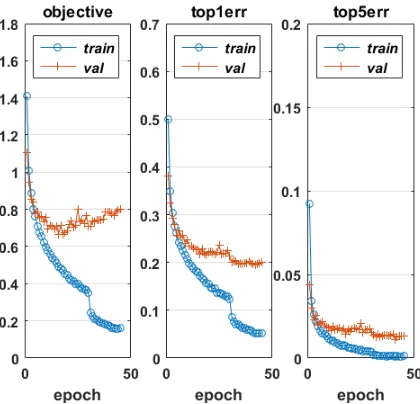
Fig. 7.2. Errors for the trained network. Horizontal axis runs over the 45 epochs of the stochastic gradient method (that is, 45 passes through the training data). Left: Circles show cost function on the training data; crosses show cost function on the validation data. Middle: Circles show the percentage of instances where the most likely classification from the network does not match the correct category, over the training data images; crosses show the same measure computed over the validation data. Right: Circles show the percentage of instances where the five most likely classifications from the network do not include the correct category, over the training data images; crosses show the same measure computed over the validation data.
probability
• 0.15 in block 1, • 0.15 in block 2, • 0.15 in block 3, • 0.35 in block 4,
• 0 in block 5 (no dropout).
We emphasize that in this case all neurons become active when the trained network is applied to the test data.
In Figure 7.2 we illustrate the training process in the case of no dropout. For the plot on the left, circles are used to show how the objective function (7.4) decreases after each of the 45 epochs. We also use crosses to indicate the objective function value on the validation data. (More precisely, these error measures are averaged over the individual batches that form the epoch—note that weights are updated after each batch.) Given that our overall aim is to assign images to one of the ten classes, the middle plot in Figure 7.2 looks at the percentage of errors that take place when we classify with the highest probability choice. Similarly, the plot on the right shows the percentage of cases where the correct category is not among the top five. We see from Figure 7.2 that the validation error starts to plateau at a stage where the stochastic gradient method continues to make significant reductions on the training error. This gives an indication that we are overfitting—learning fine details about the training data that will not help the network generalize to unseen data.
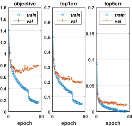
Fig. 7.3.As for Figure 7.2 in the case where dropout was used.
validation errors are of a similar magnitude. However, two key features in the dropout case are that (a) the validation error is below the training error, and (b) the validation error continues to decrease in sync with the training error, both of which indicate that the optimization procedure is extracting useful information over all epochs.
Figure 7.4 gives a summary of the performance of the trained network with no dropout (after 45 epochs) in the form of aconfusion matrix. Here, the integer value in the general i, j entry shows the number of occasions where the network predicted category i for an image from categoryj. Hence, off-diagonal elements indicate mis-classifications. For example, the (1,1) element equal to 814 in Figure 7.4 records the number of airplane images that were correctly classified as airplanes, and the (1,2) element equal to 21 records the number of automobile images that were incorrectly classified as airplanes. Below each integer is the corresponding percentage, rounded to one decimal place, given that the test data has 1,000 images from each category. The extra row, labeled “all”, summarizes the entries in each column. For example, the value 81.4% in the first column of the final row arises because 814 of the 1,000 airplane images were correctly classified. Beneath this, the value 18.6% arises because 186 of these airplane images were incorrectly classified. The final column of the matrix, also labeled “all”, summarizes each row. For example, the value 82.4% in the final column of the first row arises because 988 images were classified by the network as airplanes, with 814 of these classifications being correct. Beneath this, the value 17.6% arises because the remaining 174 out of these 988 airplane classifications were incorrect. Finally, the entries in the lower right corner summarize over all categories. We see that 80.1% of all images were correctly classified (and hence 19.9% were incorrectly classified).
Fig. 7.4. Confusion matrix for the the trained network from Figure 7.2.
sampled from those that were misclassified by the non-dropout network.
8. Of Things Not Treated. This short introductory article is aimed at those who are new to deep learning. In the interests of brevity and accessibility we have ruthlessly omitted many topics. For those wishing to learn more, a good starting point is the free online book [27], which provides a hands-on tutorial style description of deep learning techniques. The survey [23] gives an intuitive and accessible overview of many of the key ideas behind deep learning, and highlights recent success stories. A more detailed overview of the prize-winning performances of deep learning tools can be found in [30], which also traces the development of ideas across more than 800 references. The review [36] discusses the pre-history of deep learning and explains how key ideas evolved. For a comprehensive treatment of the state-of-the-art, we rec-ommend the book [11] which, in particular, does an excellent job of introducing fun-damental ideas from computer science/discrete mathematics, applied/computational mathematics and probability/statistics/inference before pulling them all together in the deep learning setting. Those references, [11, 23, 27, 30, 36], also give a feel for the range of applications that have been tackled. The recent review article [3] focuses on optimization tasks arising in machine learning. It summarizes the current theory underlying the stochastic gradient method, along with many alternative techniques. Those authors also emphasize that optimization tools must be interpreted and judged carefully when operating within this inherently statistical framework. Leaving aside the training issue, a mathematical framework for understanding the cascade of linear and nonlinear transformations used by deep networks is given in [25].
Fig. 7.5.Confusion matrix for the the trained network from Figure 7.3, which used dropout.
[image:23.612.144.384.389.622.2]Why use artificial neural networks? Looking at Figure 2.4, it is clear that there are many ways to come up with a mapping that divides the x-y axis into two regions; a shaded region containing the circles and an unshaded region con-taining the crosses. Artificial neural networks provide one useful approach. In real applications, success corresponds to a small generalization error; the mapping should perform well when presented with new data. In order to make rigorous, general, statements about performance, we need to make some assumptions about the type of data. For example, we could analyze the situ-ation where the data consists of samples drawn independently from a certain probability distribution. If an algorithm is trained on such data, how will it perform when presented withnew data from the same distribution? The au-thors in [16] prove that artificial neural networks trained with the stochastic gradient method can behave well in this sense. Of course, in practice we can-not rely on the existence of such a distribution. Indeed, experiments in [37] indicate that the worst case can be as bad as possible. These authors tested state-of-the-art convolutional networks for image classification. In terms of the heuristic performance indicators used to monitor the progress of the train-ing phase, they found that the stochastic gradient method appears to work just as effectively when the images are randomly re-labelled. This implies that the network is happy to learn noise—if the labels for the unseen data are similarly randomized then the classifications from the trained network are no better than random choice. Other authors have established negative results by showing that small and seemingly unimportant perturbations to an image can change its predicted class, including cases where one pixel is altered [33]. Related work in [4] showed proof-of-principle for anadversarial patch, which alters the classification when added to a wide range of images; for example, such a patch could be printed as a small sticker and used in the physical world. Hence, although artificial neural networks have outperformed rival methods in many application fields, and seem particularly well-suited for computer vision, speech and audio recognition, natural language processing, image segmentation, regression, imputing missing data and playing board games, the reasons behind this success are not fully understood. The sur-vey [35] describes a range of mathematical approaches that are beginning to provide useful insights, whilst the discussion piece [26] includes a list of ten concerns.
Which nonlinearity? The sigmoid function (2.1), illustrated in Figure 2.2, and the rectified linear unit (7.3) are popular choices for the activation function. Alternatives include thestep function,
0, forx≤0, 1, forx >0.
Each of these can undergo saturation: produce very small derivatives that thereby reduce the size of the gradient updates. Indeed, the step function and rectified linear unit have completely flat portions. For this reason, a leaky rectified linear unit, such as,
f(x) =
0.01x, forx≤0, x, forx >0,
inputs. The back propagation algorithm described in section 5 carries through to general activation functions.
How do we decide on the structure of our net? Often, there is a natural choice for the size of the output layer. For example, to classify images of individual handwritten digits, it would make sense to have an output layer consisting of ten neurons, corresponding to 0,1,2, . . . ,9, as used in Chapter 1 of [27]. In some cases, a physical application imposes natural constraints on one or more of the hidden layers [5, 17]. However, in general, choosing the overall number of layers, the number of neurons within each layer, and any con-straints involving inter-neuron connections, is not an exact science. Rules of thumb have been suggested, but there is no widely accepted technique. In the context of image processing, it may be possible to attribute roles to different layers; for example, detecting edges, motifs and larger structures as informa-tion flows forward [23], and our understanding of biological neurons provides further insights [11]. But specific roles cannot be completely hardwired into the network design—the weights and biases, and hence the tasks performed by each layer, emerge from the training procedure. We note that the use of back propagation to compute gradients is not restricted to the types of con-nectivity, activation functions and cost functions discussed here. Indeed, the method fits into a very general framework of techniques known asautomatic differentiation oralgorithmic differentiation [14].
How big do deep learning networks get? The AlexNet architecture [22] achieved groundbreaking image classification results in 2012. This network used 650,000 neurons, with five convolutional layers followed by two fully connected lay-ers and a final softmax. The programmeAlphaGo, developed by the Google DeepMind team to play the board game Go, rose to fame by beating the hu-man European champion by five games to nil in October 2015 [31]. AlphaGo makes use of two artificial neural networks with 13 layers and 15 layers, some convolutional and others fully connected, involving millions of weights. We emphasize that for the large number of parameters used by such deep net-works, over 100 Million in some cases, correspondingly large data sets must be available and the overfitting issue looms large.
Didn’t my numerical analysis teacher tell me never to use steepest descent? It is known that the steepest descent method can perform poorly on exam-ples where other methods, notably those using information about the second derivative of the objective function, are much more efficient. Hence, opti-mization textbooks typically downplay steepest descent [10, 28]. However, it is important to note that training an artificial neural network is a very specific optimization task:
• the problem dimension, and the expense of computing the objective function and its derivatives, can be extremely high,
• the optimization task is set within a framework that is inherently sta-tistical in nature,
• a great deal of research effort has been devoted to the development of practical improvements to the basic stochastic gradient method in the deep learning context.
on information from previous iterates. Competing aims of such adaptive approaches are (i) to learn the overall scale of the problem, (ii) to avoid slow progress, and (iii) to converge to a local minimum of the underlying cost function. In addition, many variations of the stochastic gradient step have been developed that make use of previous information more directly. From a theoretical perspective, results that guarantee convergence of the stochastic gradient method typically assume that the learning rate tends to zero as the iteration progresses. For example, denoting the learning rate on iterationk byηk, a typical convergence proof requires
∞ X
k=1
η2k (8.1)
to be finite. Intuitively, this constraint helps to avoid the circumstance where the method bounces around the minimum as the gradient sample changes from step to step.
A promising line of research is to connect the stochastic gradient method with discretizations of stochastic differential equations, [32], generalizing the idea that many deterministic optimization algorithms can be viewed as timestep-ping methods for computing steady states of gradient ODEs, [18]. This per-spective, whereηk is regarded as a timestep, also helps to motivate a second
requirement that is often imposed alongside finiteness of (8.1) in asymptotic convergence proofs—we need the overall “time interval”
∞ X
k=1
ηk
to be infinite in order for the method to have a chance of picking up the long-time behavior.
We also remark that the introduction of more traditional tools from the field of optimization is leading to new classes of training algorithms. We refer to [3] for the state-of-the art in algorithm development and convergence theory, while noting that a theoretical underpinning for the success of the stochastic gradient method in training networks is far from complete.
Is it possible to regularize? As we discussed in section 7, overfitting occurs when a trained network performs accurately on the given data, but cannot general-izewell to new data. Regularization is a broad term that describes attempts to avoid overfitting by rewarding smoothness. One approach is to alter the cost function in order to encourage small weights. For example, (3.3) could be extended to
Cost = 1 N
N X
i=1 1 2ky(x
{i})−a[L](x{i})k2 2+
λ N
L X
l=2
kW[l]k2
2. (8.2)
What about ethics and accountability? The use of “algorithms” to aid decision-making is not a recent phenomenon. However, the increasing influence of black-box technologies is naturally causing concerns in many quarters. The recent articles [8, 15] raise several relevant issues and illustrate them with concrete examples. They also highlight the particular challenges arising from massively-parameterized artificial neural networks. Professional and govern-mental institutions are, of course, alert to these matters. In 2017, the Asso-ciation for Computing Machinery’s US Public Policy Council released seven Principles for Algorithmic Transparency and Accountability1. Among their recommendations are that
• “Systems and institutions that use algorithmic decision-making are en-couraged to produce explanations regarding both the procedures fol-lowed by the algorithm and the specific decisions that are made”, and • “A description of the way in which the training data was collected should
be maintained by the builders of the algorithms, accompanied by an exploration of the potential biases induced by the human or algorithmic data-gathering process.”
Article 15 of the European Union’s General Data Protection Regulation 2016/6792, which took effect in May 2018, concerns “Right of access by the
data subject,” and includes the requirement that “The data subject shall have the right to obtain from the controller confirmation as to whether or not personal data concerning him or her are being processed, and, where that is the case, access to the personal data and the following information:.”Item (h) on the subsequent list covers
• “the existence of automated decision-making, including profiling, refered to in Article 22(1) and (4) and, at least in those cases, meaningful in-formation about the logic involved, as well as the significance and the envisaged consequences of such processing for the data subject.” What are some current research topics? Deep learning is a fast-moving,
high-bandwidth field, where many new advances are driven by the needs of specific application areas and the features of new high performance computing archi-tectures. Here, we briefly mention three hot-topic areas that have not yet been discussed.
Training a network can be an extremely expensive task. When a trained network is seen to make a mistake on new data, it is therefore tempting to fix this with a local perturbation to the weights and/or network structure, rather than re-training from scratch. Approaches for this type of on the fly tuning can be developed and justified using the theory of measure concentration in high dimensional spaces [13].
Adversarial networks, [12], are based on the concept that an artificial neural network may be viewed as agenerative model: a way to create realistic data. Such a model may be useful, for example, as a means to produce realistic sentences, or very high resolution images. In the adversarial setting, the generative model is pitted against a discriminative model. The role of the discriminative model is to distinguish between real training data and data produced by the generative model. By iteratively improving the performance of these models, the quality of both the generation and discrimination can be
1https://www.acm.org/
increased dramatically.
The idea behind autoencoders [29] is, perhaps surprisingly, to produce an overall network whose output matches its input. More precisely, one network, known as the encoder, corresponds to a map F that takes an input vector, x ∈ Rs, and produces a lower dimensional output vector F(x) ∈ Rt. So
ts. Then a second network, known as thedecoder, corresponds to a map G that takes us back to the same dimension as x; that is, G(F(x)) ∈ Rs.
We could then aim to minimize the sum of the squared errorkx−G(F(x))k2 2
over a set of training data. Note that this technique does not require the use of labelled data—in the case of images we are attempting to reproduce each picture without knowing what it depicts. Intuitively, a good encoder is a tool for dimension reduction. It extracts the key features. Similarly, a good decoder can reconstruct the data from those key features.
Where can I find code and data? There are many publicly available codes that provide access to deep learning algorithms. In addition to MatConvNet [34], we mention Caffe [20], Keras [6], TensorFlow [1], Theano [2] and Torch [7]. These packages differ in their underlying platforms and in the extent of expert knowledge required. Your favorite scientific computing environment may also offer a range of proprietary and user-contributed deep learning tool-boxes. However, it is currently the case that making serious use of modern deep learning technology requires a strong background in numerical comput-ing. Among the standard benchmark data sets are the CIFAR-10 collection [21] that we used in section 7, and its big sibling CIFAR-100, ImageNet [9], and the handwritten digit database MNIST [24].
Acknowledgements. We are grateful to the MatConvNet team for making their package available under a permissive BSD license. The MATLAB code in List-ings 6.1 and 6.2 is available as on-line supplementary material. EPSRC Data State-ment: original MATLAB code associated with this article can be accessed via the Supplementary Materials. Other code and data used in this article is available in the public domain, as indicated in the text.
REFERENCES
[1] M. Abadi, P. Barham, J. Chen, Z. Chen, A. Davis, J. Dean, M. Devin, S. Ghemawat, G. Irving, M. Isard, M. Kudlur, J. Levenberg, R. Monga, S. Moore, D. G. Murray, B. Steiner, P. Tucker, V. Vasudevan, P. Warden, M. Wicke, Y. Yu, and X. Zheng, TensorFlow: A system for large-scale machine learning, in 12th USENIX Symposium on Operating Systems Design and Implementation (OSDI 16), 2016, pp. 265–283.
[2] R. Al-Rfou, G. Alain, A. Almahairi, C. Angermueller, D. Bahdanau, N.