Use of Turbine-level Data for Improved Wind
Power Forecasting
Jethro Browell,
Member, IEEE
, Ciaran Gilbert,
Student Member, IEEE
and David McMillan,
Member, IEEE
University of Strathclyde, Glasgow, UK
{
jethro.browell, ciaran.gilbert, d.mcmillan
}
@strath.ac.uk
c
2017 IEEE. Personal use of this material is permitted. Permission from IEEE must be obtained for all other uses, in any current or future media, including reprinting/republishing this material for advertising or promotional purposes, creating new collective works, for resale or redistribution to servers or lists, or reuse of any copyrighted component of this work in other works. This work has been accepted for publication in the proceedings of the IEEE PowerTech Conference, Manch-ester, UK, 2017.
Abstract—Short-term wind power forecasting is based on mod-elling the complex relationship between the weather forecasts and wind farm power production. To date, efforts to improve wind power forecasts have focused on improving Numerical Weather Prediction and wind farm power curve models. However, utility-scale wind farms cover large areas meaning that a single power curve model may struggle to represent the collective behaviour of large numbers of wind turbines. Contemporary statistical techniques are capable of processing large volumes of data, enabling the assimilation of measurements from individual wind turbines to construct a more detailed representation of wind farm power generation. Here, three state-of-the-art techniques are applied to forecast wind farm power production 1) directly from numerical weather predictions, and 2) by aggregating forecasts for individual wind turbines. Furthermore, it is observed that some wind turbines are better predictors than others and an aggregation process based on conditional weighting is proposed. In case studies of two large wind farms in the UK, it is shown that wind farm power forecasts comprising a conditional weighted sum of turbine-level predictions are superior to a direct wind farm forecast for horizons up to 48 hours ahead. Specifically, performance of the best-performing benchmark, the gradient boosting machine, is improved by 12% at Clyde South wind farm and by 6% at Gordonbush.
Index Terms—Wind Power Forecasting, Big Data, Machine Learning, LASSO, Gradient Boosting
I. INTRODUCTION
Wind power forecasting is an integral component of modern power system operation and electricity market participation in areas with a significant penetration of wind generation. The stochastic nature of the wind resource means that forecasts are required to inform decisions where future generation is a factor. Forecast from days to a week ahead are valuable when scheduling conventional generation and maintenance on wind farms, day-ahead forecasts are required for participants in electricity markets, and intra-day forecasts are used by par-ticipants in short-term markets and to power system operators who must balance supply and demand in real time [1], [2].
Deterministic wind power forecasting, comprising single-valued estimates of future power, is approaching technological maturity following a concerted research effort reviewed com-prehensively in [3], [4]. At present there are many commercial providers offering deterministic wind power forecasts. How-ever, there is a broad consensus in the academic community that wind power should be modelled as a stochastic process and that forecasts should be probabilistic in order to quantify forecast uncertainty [5], [6]. That said, many forecast users still only utilise single-valued forecasts due to the difficulty of incorporating complex probabilistic information into decision-making processes in practice.
There are two sources of error in wind power forecasting: meteorological forecast errors, and errors introduced by the wind-to-power conversion process. In this work we attempt to reduce the later. Typically, wind-to-power conversion is modelled at the farm level; these models may contain tens or hundreds of input features derived from meteorological fore-casts and lagged measurements. Approaches based on boosted regression trees [7], [8], linear regression with sparsity [9] and neural networks [10] are at the forefront of the technology, with gradient boosting methods winning both the 2012 and 2014 Global Energy Forecasting Competitions [11], [12]. However, large wind farms contain many turbines distributed over a wide geographical area with each turbine experiencing different conditions. Here we investigate the utilisation of turbine-level power production an propose a bottom-up hier-archical forecasting methodology, an idea which has proved successful in other applications [13]–[15].
The power generated by wind turbines is routinely measured and transmitted to operators making this data available for use in forecasting systems. Here, we test the hypothesis that power forecasts for large wind farms can be improved by modelling and combining the wind-to-power conversion process for individual spatially distributed turbines. We will draw upon developments in large-scale spatio-temporal forecasting such as [16], [17] and investigate the ability of modern machine learning algorithms to efficiently model these processes and aggregate the resulting forecasts.
II. FORECASTINGMETHODOLOGY
on NWP and lagged power measurements and then aggregated to form a prediction of the total wind farm production. Forecasts are produced from 30 minutes to 48 hours ahead in 30 minute intervals.
Three state-of-the-art forecasting techniques are imple-mented to forecast wind farm and wind turbine power produc-tion. First is linear regression with sparse parameter estimation using the least absolute shrinkage and selection operator (LASSO) [18]. LASSO simultaneously performs parameter estimation and feature selection enabling the user to engineer many features and then rely on the estimator todeselectsome features with parameters estimates equalling exactly zero. Second is the gradient boosting machine (GBM) [19] which is a tree-based method for non-linear function approximation, and third is the extreme gradient boosting machine, which is an extension of the GBM [20]. The LASSO and GBM have pedigree as the basis of winning entries in the wind power forecasting track of the Global Energy Forecasting Competition 2014, and the latter in particular for winning many other machine learning competitions [12].
A. Least Squares LASSO
A linear model for the quantityytwe are attempting to fore-cast is the weighted sum of input features xt= [x1,t, ..., xp,t] plus an error term t,
yt= p
X
i=1
βixi,t+t , (1) where β = [β1, ..., βp]T are unknown parameters to be estimated.
For a set ofT samples,{Y,X}, whereYandXare matri-ces of vertically stacked instanmatri-ces of yt andxt, respectively, the least squares estimate ofβ is the solution to the problem
argmin
β
||Y−Xβ||2
2 . (2)
Large numbers of features, and possible multicollinearity, and can lead to poor parameter estimates and predictive perfor-mance, as well as making model interpretation difficult [18]. There is therefore a need to regularise the estimation process. LASSO achieves this by penalising the `1 norm of β. The lasso estimation problem is given by
argmin
β
1
2T||Y−Xβ||
2
2+λ||β||1
. (3)
The user-defined shrinkage parameterλcontrols sparsity and is typically selected via a cross-validation procedure.
Due to the non-linear nature of the relationship between wind speed and power, and others, it is necessary to construct features which capture these effects. This can be achieved by recasting (1) as an additive model
yt= p
X
i=1
βifi(xi,t) +t , (4) wherefi(·)are smooth functions chosen to capture non-linear effects such as the familiar power curve. The capability of
LASSO to perform feature selection makes this convenient as multiple functionsfi(·)can be included but only those which add the most value are retained in the final model.
B. Tree-based Gradient Boosting Machine
A regression tree with J leaves and weights wj has the additive form
k(x;T ={wj, Rj}J) = J
X
j=1
wjI(x∈Rj) (5)
where Rj are disjoint regions that collectively cover the input space spanned byx, and I(·) is the indicator function. Individual trees can be fit very efficiently using the a process of recursive partitioning but have limited predictive power and for this reason are often called weak learners [21]. Gradient boosting attempts to overcomes this drawback by constructing a ‘stronger’ learner from an ensemble of weak learners.
The gradient boosting machineFn(xt)is the sum ofnweak learners
yt = Fn(xt) +t (6)
=
n
X
i=1
fi(xt) +t (7)
where, in this case, each fi(xt) is a regression tree. The ensemble of regression trees is constructed sequentially by estimating the new regression treefn+1(xt) via
argmin
fn+1
X
t
L(yt, Fn(xt) +fn+1(xt)) (8)
for some loss functionL(·). Where L(·)is differentiable, this optimisation can be solved by steepest descent written
gn(xt) =
∂L(yt, Fn(xt))
∂Fn
(9)
fn+1(xt) = −ρngn(xt) (10) where
ρn= argmin ρ
X
t
L(yt, Fn(xt)−ρgn(xt)) . (11)
For a finite dataset, a regression treek(x;T)is fit to the psudo-residualsgn(xt)by solving
argmin
T,γ
X
t
[−gn(xt) +γk(xt;T)] 2
. (12)
C. Extreme Gradient Boosting Machines
A recent advance gradient boosting has seen the devel-opment of Extreme Gradient Boosting (XGBoost) algorithm, which solves the optimisation problem (8) by performing sec-ond order gradient descent [20]. This approach results in more efficient model fitting making it more scalable than traditional gradient boosting, and is included here for comparison. For details of the fitting algorithm see [20].
III. WINDPOWERFORECASTING
As a benchmark, the methodologies described above are im-plemented to produce power forecasts for wind farms directly, the conventional approach to wind power forecasting, where
yt is the total power produced by the wind farm at time t. Motivated by knowledge that wind conditions can vary sig-nificantly across large wind farms and intuition that different turbines will be better predictors than others at different times, we use the same methodologies to forecast production for individual wind turbines which are then combined to produce a farm-level forecast. In both cases xt contains features from NWP, namely wind speed and direction at 10m, 80m and 100m above ground linearly interpolated to 30-minute resolution, and lagged power measurements for the most recent 48 half-hour periods. Bilinear interpolation is used to obtain single values for each meteorological variable at the location of the target wind farm from the closes four NWP grid points.
In order to capture non-linear features of the wind-power relationship in the linear model (4) a series of threshold functions are also included. Specifically
fmax(c)(xi,t) = max{c, xi,t} , c= 2,4, ...,24 . (13) These additional features are not used in the tree-methods as they would be redundant. In all models time-of-day features included to capture and diurnal bias in the NWP and are modelled by cubic spline kernels, along similar lines to [22].
A. Aggregating Turbine-level Forecasts
Two approaches to forecast aggregation are considered for the novel turbine level methodology. In the first, the forecast for the wind farm as a whole is given by the weighted sum of individual turbine forecasts. The second is also based on a weighted sum of individual turbine forecasts but in this case the weights are conditioned on the forecast wind direction. This approach was driven by the idea that different combinations of turbines will be better predictors of total wind farm generation depending on the incident wind direction due to the array layout and local topographic effects. For the simple weighted sum (WS)
yt= N
X
i=1
βixi,t+t (14)
where herexi,tis the forecasts power a theith turbine at time
t and the parametersβi are estimated by the LASSO (3). In order to condition the weighting on wind direction, separate parameters are estimated for different wind directions
N
NNE
ENE
E
ESE
SSE S
SSW WSW W
WNW NNW
0% 5% 10% 15%
Frequency
Wind Speed (m/s)
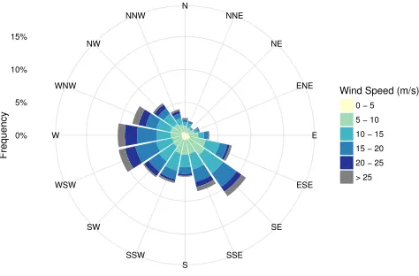
[image:3.612.318.554.60.215.2]0 − 5 5 − 10 10 − 15 15 − 20 20 − 25 > 25
Fig. 1. Wind rose for forecast wind speed and meteorological wind direction at 100m above ground for Clyde South from training dataset.
N NNE
NE
ENE
E
ESE
SE
SSE S SSW SW WSW W
WNW NW
NNW
0% 5% 10% 15%
Frequency
Wind Speed (m/s)
0 − 5 5 − 10 10 − 15 15 − 20 20 − 25 > 25
Fig. 2. Wind rose for forecast wind speed and meteorological wind direction at 100m above ground for Gordonbush from training dataset.
and the weighted sum (14) becomes the conditional weighted sum (CWS)
yt= N
X
i=1
ωi(θ)xi,t+t . (15) For practical reasons, data are grouped into a fixed number of bins (determined byk-fold cross-validation) andωi(θ)are estimated for each bin. Parameters are then estimated by
ω(θ) = argmin
β 1
2T||Yθ−Xθβ||
2
2+λ||β||1
(16)
whereYθ andXθare matrices of vertically stacked instances of yt andxt where the forecast wind direction at time t lies in the same bin asθ.
IV. CASESTUDY
[image:3.612.317.554.277.433.2]system and the wind farm power export meter are used at 30 minute resolution with instances of curtailment flagged and excluded from the forecasting exercise. Numerical Weather Forecasts from the Global Forecasting System [23] are used and comprise wind speed and direction at 80m and 100m above ground. The methodologies described are implemented in Rusing the packages glmnet,gbm, andxgboost[20], [24]–[26].
V. RESULTS
The LASSO, GBM, and XGBoost predictors and set-up to 1) forecast wind farm power production directly, and 2) forecast the power production of individual turbines. In the second case, the forecast for the wind farm as a whole is produced by a simple weighted sum (WS) and alternatively a conditional weighted sum (CWS) of turbine forecasts, with weights estimated using least squares LASSO.
To evaluate forecasts performance two metrics were used: the mean absolute error (MAE) and root mean squared error (RMSE). The RMSE across all forecast horizons was used to inform model selection and performance is evaluated by hori-zon in order to illustrate how forecast performance degrades with lead-time. These metrics are given by
MAE= 1
N
N
X
i=1
|yi−yˆi| (17)
RMSE=
v u u t
1
N
N
X
i=1
(yi−yˆi) 2
(18)
whereyˆi is the forecast ofyi.
The parameters governing the fitting process of each fore-cast method and the number of direction bins were determined by k-fold cross validation with five folds on the training data for each wind farm. The resulting direction bins are illustrated in Figure 1 and Figure 2 for each wind farm.
The computational time for 5-fold cross-validation at Gor-donbush was 6, 880, and 300 seconds for the LASSO, GBM, and XGBoost, respectively. This illustrates the important trade-off between model accuracy and computational time between each of the methodologies. Additionally, the GBM and ex-treme gradient boosting machine methods may controlled by several parameters (including learning rate, interaction depth and number of trees) whereas the only parameter for cross-validation in the LASSO is the shrinkage.
Performance of the LASSO, GBM, and XGBoost methods are plotted in Figure 3 for Clyde South. The performance of all three methods is improved across all horizons when utilising turbine-level information with the conditional weighted-sum method. At this wind farm both variants of boosted machines perform similarly with the turbine level data included up to a horizon of 24h, with the GBM method performing best overall when performance is averaged across all forecast horizons. Full results are listed in Table II. The most improved method with the incorporation of the turbine level data is the LASSO model which shows a 17% reduction in RMSE when averaged
Horizon [hours]
RMSE [% of Nominal]
0 6 12 18 24 30 36 42 48
5
10
15
20
25
[image:4.612.316.552.54.226.2]Lasso − F Lasso − CWS GBM − F GBM − CWS XGBoost − F XGBoost − CWS
Fig. 3. Forecast performance at Clyde South based on wind farm level data only (–F) and wind turbine level data with a conditional weighted sum (– CWS).
Horizon [hours]
RMSE [% of Nominal]
0 6 12 18 24 30 36 42 48
10
15
20
25
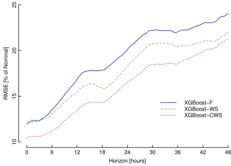
XGBoost−F XGBoost−WS XGBoost−CWS
Fig. 4. Forecast performance at Clyde South for the XGBoost method based on wind farm level data only (–F), turbine level data with a weighted sum (–WS), and wind turbine level data with a conditional weighted sum (–CWS).
across all horizons. Results for all methods are tabulated in Table III.
The value of conditioning the aggregation of individual turbine forecasts on wind direction is illustrated in Figure 4 which examines the XGBoost methodology at Clyde South. Here the simple weighted sum performs well compared to the wind farm level data and gives an appreciable improvement across forecast horizons beyond 3 hours. However, the greater value of the turbine level approach is realised through the con-ditional weighted sum method which demonstrates consistent improvement across all horizons compared to the wind farm level data only. Averaged across all forecast horizons it leads to a 16% reduction in the RMSE and 12% in MAE compared to the standard wind farm level approach.
[image:4.612.313.551.283.454.2]TABLE I
DETAILS OF WIND FARMS USED IN CASE STUDY. TRAINING AND TEST PERIODS DIFFER DUE TO DIFFERENCES IN DATA AVAILABILITY ONLY.
Wind Farm Terrain Area Number of Turbines Turbine Rating Training Period Test Period
Clyde South Complex 20km2 56 2.3MW 22 months 6 months
Gordonbush Complex 15km2 35 2MW 17 months 6 months
Horizon [hours]
RMSE [% of Nominal]
0 6 12 18 24 30 36 42 48
10
15
20
25
Lasso − F Lasso − CWS GBM − F GBM − CWS XGBoost − F XGBoost − CWS
Fig. 5. Forecast performance at Gordonbush based on wind farm level data only (–F) and wind turbine level data with a conditional weighted sum (– CWS).
South, possibly as a result of local effects which are not captured by the relatively low resolution NWP. However, the performance of all methods are improved when utilising turbine-level information, although to a lesser extent. At Clyde South the RMSE reduction was between 12% and 17% where as at Gordonbush it is between 6% and 9%. For both wind farms GBM with CWS had the lowest MAE and RMSE overall.
A summary of the results across both wind farms is shown in Table II where the error metrics have been averaged across all forecast horizons. The simple weighted sum of forecast turbine power generation led to consistent improvements in the averaged RMSE at both wind farms, with the XGBoost method showing the most improvement. However, the weighted sum of turbine forecasts conditional on wind direction improved overall performance to a greater extent across all methods and wind farms.
VI. CONCLUSIONS
The use of turbine level data for improved wind forecasting has been studied and evaluated using a case study of two wind farms with differing characteristics. Three state-of-the-art techniques — linear regression (additive model) estimated via LASSO, gradient boosting machines, and extreme gradient boosting machines — were applied to forecast wind farm power production directly from numerical weather predictions, and by aggregating forecasts made in the same way but for individual wind turbines.
On a case study comprising two large wind farms consider-ing forecast up to 48 hours ahead, it is shown that aggregatconsider-ing
TABLE II
SUMMARY RESULTS FOR DIRECT WIND FARM LEVEL FORECASTS(F), TURBINE LEVEL WITH WEIGHTED SUM(WS),AND TURBINE LEVEL WITH
CONDITIONAL WEIGHTED SUM(CWS). THE BEST PERFORMING AGGREGATION METHOD FOR EACH FORECASTING APPROACH IS ITALICISED,AND BEST OVERALL PERFORMANCES ARE EMBOLDENED.
Model Aggregation Clyde South Gordonbush
RMSE MAE RMSE MAE
LASSO
F 20.69 14.33 20.20 15.21
WS 20.63 14.62 20.16 15.59
CWS 17.16 12.76 18.68 14.76
GBM
F 17.74 12.70 18.57 13.76
WS 17.61 12.44 18.53 13.98
CWS 15.62 11.19 17.40 13.25
XGBoost
F 19.19 13.55 19.88 14.63
WS 17.77 12.97 18.93 14.60
CWS 16.06 11.96 18.02 14.05
Units: Percentage of nominal capacity.
TABLE III
PERCENTAGE REDUCTION INRMSECOMPARED TO DIRECT WIND FARM FORECASTS FOR AGGREGATED TURBINE LEVEL FORECASTS WITH WEIGHTED SUM(WS),AND CONDITIONAL WEIGHTED SUM(CWS)
Model Aggregation Clyde South Gordonbush
LASSO WS 0.29 0.20
CSW 17.05 7.52
GBM WS 0.68 0.20
CWS 11.94 6.30
XGBoost WS 7.37 4.74
CWS 16.33 9.36
turbine-level forecasts gives an improved overall wind farm production forecast. Furthermore, the aggregation process is improved if conditioned on wind direction. It was found that gradient boosting machine produced forecasts with the lowest RMSE and MAE, reducing RMSE over direct wind farm-level forecasting by 12% for the Clyde South wind farm, and 6% for Gordonbush, which has a more complex wind rose.
Future work should consider the utility of this approach in combination with downscaled NWP and if similar improve-ments are possible on very-short time scales where statistical methods typically out perform those based on NWP. Another consideration should be the use of turbine-level forecasting in a probabilistic setting.
ACKNOWLEDGEMENTS
EPSRC Doctoral Prize, grant number EP/M508159/1, and Ciaran Gilbert by the University of Strathclyde’s EPSRC Centre for Doctoral Training in Wind and Marine Energy Systems, grant number EP/L016680/1.
Data Statement: Due to confidentiality agreements with research collaborators, access to wind power data is restricted. Numerical weather predictions are from GFS and are available atwww.ncdc.noaa.gov.
REFERENCES
[1] T. Ackermann, Ed.,Wind power in power systems, 2nd ed. John Wiley & Sons: New York, 2012.
[2] J. Morales, A. Conejo, H. Madsen, P. Pinson, and M. Zugno,Integrating Renewable in Electricity Markets. Springer, 2014.
[3] C. Monteiro, R. Bessa, V. Miranda, A. Botterud, J. Wang, and G. Conzel-mann, “Wind power forecasting: State-of-the-art 2009,” Argonne Na-tional Laboratory ANL/DIS-10-1, Tech. Rep., 2009.
[4] G. Giebel, R. Brownsword, G. Kariniotakis, M. Denhard, and C. Draxl,The State-of-the-Art in Short-Term Prediction of Wind Power. ANEMOS.plus, 2011, project funded by the European Commission under the 6th Framework Program, Priority 6.1: Sustainable Energy Systems.
[5] P. Pinson, “Wind energy: Forecasting challenges for its operational management,”Statistical Science, vol. 28, no. 4, pp. 564–585, 2013. [6] Y. Zhang, J. Wang, and X. Wang, “Review on probabilistic forecasting
of wind power generation,” Renewable and Sustainable Energy Reviews, vol. 32, no. 0, pp. 255–270, 2014. [Online]. Available: http://www.sciencedirect.com/science/article/pii/S1364032114000446 [7] L. Silva, “A feature engineering approach to wind power forecasting:
{GEFCom}2012,”International Journal of Forecasting, vol. 30, no. 2, pp. 395–401, 2014.
[8] M. Landry, T. P. Erlinger, D. Patschke, and C. Varrichio, “Probabilistic gradient boosting machines for GEFCom2014 wind forecasting,” Inter-national Journal of Forecasting, vol. 32, no. 3, pp. 1061–1066, 2016. [9] F. Ziel, C. Croonenbroeck, and D. Ambach, “Forecasting wind power —
modeling periodic and non-linear effects under conditional heteroscedas-ticity,”Applied Energy, vol. 177, pp. 285–297, 2016.
[10] D. Lee and R. Baldick, “Short-term wind power ensemble prediction based on gaussian processes and neural networks,”Smart Grid, IEEE Transactions on, vol. 5, no. 1, pp. 501–510, Jan 2014.
[11] T. Hong, P. Pinson, and S. Fan, “Global energy forecasting competition 2012,”International Journal of Forecasting, vol. 30, pp. 357–363, 2014.
[12] T. Hong, P. Pinson, S. Fan, H. Zareipour, A. Troccoli, and R. J. Hyndman, “Probabilistic energy forecasting: Global energy forecasting competition 2014 and beyond,” International Journal of Forecasting, 2016, in press.
[13] B. J. Dangerfield and J. S. Morris, “Top-down or bottom-up: Aggregate versus disaggregate extrapolations,” International Journal of Forecast-ing, vol. 8, pp. 233–241, 1992.
[14] R. J. Hyndman, R. A. Ahmed, G. Athanasopoulos, and H. L. Shang, “Optimal combination forecasts for hierarchical time series,” Computa-tional Statistics & Data Analysis, vol. 55, no. 9, pp. 2579–2589, 2011. [15] T. Hong, P. Wang, and L. White, “Weather station selection for electric load forecasting,”International Journal of Forecasting, vol. 31, no. 2, pp. 286–295, 2015.
[16] J. Dowell and P. Pinson, “Very-short-term probabilistic wind power forecasts by sparse vector autoregression,”IEEE Transactions on Smart Grid, vol. 7, no. 2, pp. 763–770, March 2016.
[17] R. Bessa, A. Trindade, A. Monteiro, V. Miranda, and C. S. P. Silva, “Solar power forecasting in smart grid using distributed information,” in18th Power Systems Computation Conference, 2014.
[18] T. Hastie, R. Tibshirani, and M. Wainwright,Statistical Learning with Sparsity: the Lasso and Generalizations, ser. Monographs on Statistics & Applied Probability. Chapman and Hall/CRC, 2015.
[19] J. Friedman, “Greedy function approximation: a gradient boosting ma-chine,”Annals of Statistics, vol. 29, no. 5, pp. 1189–1232, 2001. [20] T. Chen and C. Guestrin, “XGBoost: A Scalable Tree Boosting System,”
ArXiv e-prints, June 2016.
[21] L. Breiman, J. Friedman, C. J. Stone, and R. Olshen,Classification and Regression Trees. Chapman & Hall/CRC, 1984.
[22] F. Ziel, R. Steinert, and S. Husmann, “Efficient modeling and forecasting of the electricity spot price,” Energy Economics, vol. 47, pp. 98–111, 2015.
[23] NOAA National Centers for Environmental Prediction, “NOAA/NCEP Global Forecast System (GFS) Atmospheric Model,” June 2011, ac-cessed May 2016.
[24] R Core Team, R: A Language and Environment for Statistical Computing, R Foundation for Statistical Computing, Vienna, Austria, 2016. [Online]. Available: https://www.R-project.org/
[25] J. Friedman, T. Hastie, and R. Tibshirani, “Regularization paths for generalized linear models via coordinate descent,”Journal of Statistical Software, vol. 2010, no. 1, pp. 1–22, 33.