RESEARCHARTICLE
Determining the optimal spatial
and temporal thresholds that
maximize the predictive accuracy of
the prospective space-time scan
statistic (PSTSS) hotspot method
Monsuru Adepeju and Andrew Evans
School of Geography, University of Leeds, United Kingdom
Received: June 14, 2017; returned: October 15, 2017; revised: December 14, 2017; accepted: February 22, 2018.
Abstract:The spatial and temporal thresholds (KandT) are two key parameters that con-trol the performance of the prospective space-time scan statistical (PSTSS) hotspot method. This study proposes an objective function approach, in which the optimal values ofKand
T that maximize the mean hit rate (a measure of predictive accuracy), are determined. The proposed approach involves sweeping through a range of values defined for each parame-ter and monitors their impacts on the mean hit rate. A case study of the crime data sets of the South Chicago area is presented in which 100 one-day consecutive predictions are car-ried out. Two aspects of the derived results are significant. First, is that there is a trade-off between the predictive accuracy obtainable from the use of PSTSS and the level of hotspot coverage. Second, is thatKis found to have more influence on the accuracy thanT. AsK
increases in size, the accuracy level decreases, whereas there is no notable impact ofT on the accuracy, particularly whenT ≥30 days. This study also demonstrated the distinctive-ness of PSTSS as a hotspot method as compared to other conventional hotspot methods. Lastly, it is argued that the approach demonstrated in this study is not only applicable to crime hotspot prediction, but could also be used in many other domains where the PSTSS technique is used.
1
Introduction
The space-time scan statistic (STSS) is one of the most commonly used geographical surveil-lance techniques for detecting clusters of geographical phenomenon [15]. It is based on the idea of exhaustive scanning of geographical space using a continuously changing-in-size space-time window (usually represented as a cylinder), which identifies regions of unusual concentration of geographical events relative to an expected background risk for the neighborhood. Depending on the application domain, the identified regions, otherwise referred to as clusters, may be used for decision-making processes. For example, STSS has been used in the public health domain [9, 15] in order to detect the outbreak of diseases so that infected people or locations can be quarantined. A recent application of STSS is in criminology, for example using clusters of crime identified by STSS to model risk hotspots, through which police patrols can be planned. This technique of predictive hotspotting was pioneered in [3], where it was called the prospective space time scan statistic (PSTSS).
A sequel to this study was conducted by Adepeju and Cheng [1], where the spatial threshold (K) which is most appropriate for crime prediction was determined. In the PSTSS method, theKandTrepresent the fixed maximum spatial size and maximum time length, respectively, of the scanning window. Despite the growing use of the PSTSS technique across different application domains and the significant impact on computing time, the best strategy for determining the optimal value ofKand/orThas remained an open question. In epidemiology and public health applications, for which the PSTSS was originally introduced, there is a standard setting for the values ofKandT. ForK, it is set as 50% of either the population at risk or the actual geographical size of the area, where all measure-ments are based on Euclidean distance. This large percentage is generally recommended to allow clusters of both small and large sizes to be detected without any pre-selection bias. Also, forT half the length of the study period is recommended for the same reason that it will allow potential clusters of any temporal durations to be identified [15, 19]. In crime analysis these settings ofK andT have been used for detecting historical hotspots of crime [8, 16], but not for short-term crime hotspot prediction, where a daily predictive hotspot is normally used to inform decision processes like operational briefings and police patrols. A few other studies have also proposed using a rough estimate forKandTbased on the visible spatial aggregation in the data set [3, 18]. While this turned out to be a good idea in terms of faster computation, the predictive accuracy of the PSTSS, in terms of the level of true crimes predicted for a space, was very low as compared to other predictive methods. Moreover, while the major focus in the past has been on determining the best value of K, the temporal counterpart, T, has been completely ignored. Therefore, this study aims to address this research gap.
value ofKandT are carefully selected for the PSTSS technique, not only is the technique capable of capturing the RNRV but also it will result in the improved accuracy of hotspot prediction [1].
For crime, a short-term prediction involves anticipating future crime within a very small time window, such as the next one or two days [5]. These are the most relevant time win-dows for policing operations, such as patrolling and emergency response. Thus, in order to effectively capture the emerging clusters that are indicative of the most imminent future crimes, both theKandT settings have to be chosen very carefully. Yet, there has been no consensus on the best way to undergo this parameter setting. Although, the general belief is that the larger the values ofKandT, the higher the possibility there is of detecting the most relevant clusters; this ignores the fact that too many spurious clusters (false alarms) may also be included in the results. Equally, a too small value ofT may prevent the de-tection of the most relevant spatial and temporally long clusters. Hence, one objective of this study is to investigate all these assumptions and examine how they will impact the performance of the PSTSS for short-term crime hotspot prediction. Overall, the main goal is to determine the most appropriate settings forK andT, which will thus optimize the chosen performance criteria.
Generally, the evaluation of the performance of any predictive hotspot method has been a subject of debate, both within the academic and the law enforcement environment. As a complicated construct of neighborhood and population at risk, predictive hotspots (clus-ters) are almost impossible to investigate through ground-truthing. In this study, it is ar-gued that the performance of a hotspot technique should be based on intuitive meanings linked pragmatically to operational policing. For example, since a predictive hotspot is a representation of locations where imminent crimes are likely, if we overlay such imminent crimes (in retrospect) against the locations already identified as risky, the exercise should tell us how effective the hotspot is as a representation of a vulnerable location. This can therefore be referred to as thepredictive accuracyof the hotspot. This idea was originally proposed as thehit rate [5]. Furthermore, the aggregation or disaggregation of hotspot regions across an area may also be used to evaluate the amount of time required to visit all the hotspots—an idea which may be translated as easiness to patrol. A compilation of similar ideas can be found in some previous studies such as [6] and [3]. These studies mainly focused on the comparative analysis of different hotspot methods based on these performance measures.
It was highlighted in Eck et al. [11] that the choice of some predictive parameters in the presentation of a hotspot map still presents itself as a problem since most analysts fail to question the validity of estimated hotspots in achieving a preferred result. Yet, there have been very few studies on how to choose the best parameter setting to generate the most robust output, based on the performance criteria chosen. Thus, this study aims to address this research gap by focussing on the two most basic parameters of predictive hotspot algorithms—the spatial threshold and the temporal threshold—using the PSTSS as an example.
1.1
The significance of this study
This study proposes an objective function approach to determine the best values of the spatial and temporal thresholds (i.e.,K andT) for the PSTSS for crime prediction. This study is an extension of the Adepeju and Cheng [1] study to include the interplay between
K andT on the hit rate measure as the objective function to be maximized. The aim is to make recommendations on the selection strategy of these two parameters, in relation to crime data sets of different spatial and temporal characteristics during short-term crime hotspot prediction. It is argued that the result of this study will not only be relevant to crime data sets but also to other geographical data domains, where the STSS and PSTSS are being applied.
The remainder of this paper will be organized as follows. Section 2 provides a descrip-tion of the PSTSS technique in reladescrip-tion to the parametersK andT. This also includes an explanation of how the predictive hotspot is generated from the results of the PSTSS tech-nique. In Section 3 the objective function—the hit rate—is described. Section 4 presents the case study data set and the discussion of its spatial characteristics. Furthermore, the param-eter settings forKandT and the prediction and evaluation details are described. Section 5 presents a discussion of the results. Lastly, conclusions and future work are discussed in Section 6.
2
The prospective space-time scan statistic (PSTSS), and its
spatial and temporal thresholds
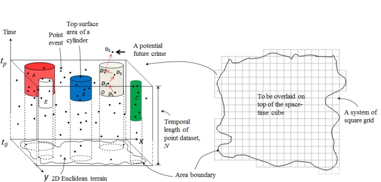
The PSTSS technique attempts to identify regions in space and time, represented by cylin-drical shapes, of elevated risks relating to a geographical point data set,N, relative to a background risk of the area [15]. The technique works by placing, on every unique point location (x,y, t), a cylinder whose width and length are continuously increasing until a maximum value ofKandTare reached along thex,ydimension andtdimension, respec-tively. Both the width and the length of a cylinder are increased systematically in such a way that the next cylinder size contains a total number crimes that is greater than that of the previous cylinder size by just one crime. By so doing, a very exhaustive scanning is en-sured. TheKandT are referred to as the maximum spatial scan extent and the maximum temporal scan extent (T), respectively. These are shortened as spatial threshold and tempo-ral threshold, respectively. A likelihood ratio,S, representing the risk level of each cylinder is calculated by comparing the observed number of events and the expected number of events within the cylinder. Lastly, all the cylinders are filtered such that only high risk, non-overlapping cylinders are reported. The non-overlapping cylinders are considered in order to simplify the results. The PSTSS has been widely applied in several fields including epidemiology [21], public health [15] and criminology [3].
The PSTSS method is distinct from the general STSS approach in that we only consider clusters continuously extending up to the present time, instead of considering all clusters, including those which are strictly separated into the past (see Figure 1a). Clusters existing up to the current time are indicative of locations where repeat victimizations are expected imminently [3].
S=
nw
µw
nw
N−nw
N−µw
N−nw
; If nw> µw, and S= 1; otherwise. (1)
Wherenwandµwrepresent, respectively, the observed and expected number of events
in the space-time regionw. We always consider spatial regions which are centred on an event and are disk shaped, while time regions always consist of intervals of time extend-ing up to the current time. By takextend-ing a Poisson approximation, we estimate the expected number of events by counting all the events in the spatial region (which occur at any time), counting all the events in the time region (which occur anywhere in space) and then mul-tiplying the two, before finally dividing by the total number of eventsN. The PSTSS as implemented in the SaTScanTM software [14] was used in this study.
At present, there is no general consensus on the most appropriate strategy for setting the value ofKandT. In this study, an optimization strategy will be introduced for determining the optimal value ofK andT, which is demonstrated to be effective for short-term crime hotspot predictions. This constitutes the major contribution of this work.
2.1
Generating the predictive hotspot maps
The generation of a predictive hotspot map from the PSTSS for short-term crime hotspot prediction is illustrated with Figure 1a. The utility of PSTSS in this respect is based on the idea that a potential future crime, say D5, will be repeated such that it matches the theory of RNRV of crime within the spatial region occupied by a clusterD. The theory of RNRV states that D5 may emerge as a consequence of the direct impacts of any of the previous crime incidents (i.e., D1, D2, . . . , D4). This idea was employed in two previously published articles [1,3], and was confirmed to possess strong potential for identifying emerging crime hotspots.
Figure 1c illustrates the resulting 2D map which is generated by overlaying a system of square grids (Figure 1b) on top of the space-time cube in Figure 1a. We work in order from the mostextremecluster (the most different to its expected value) to the least extreme cluster. For each cluster, we work outwards from the centre of the cluster, marking each grid cell which intersects the spatial region of the cluster. Once the desiredcoverage level has been reached, we stop, even if this is half-way through processing a cluster (Figure 1c). Coverage is determined by the pragmatics of policing, in the sense that only a specific percentage of an area is likely to be practical to police.
Given that the geographical events in Figure 1 are crime incidents, the shaded grid cells will represent regions at risk of being imminently victimized, according to the theory of RNRV. Starting from the mostriskygrid cell (i.e., the darkest red shade), one can highlight just the required area of interest for hotspot coverage. For example, in Figure 1c, the rank-ing process is top-sliced partway through the fillrank-ing of the brown circle, givrank-ing a hotspot coverage of approximately 20%; calculated as the number of selected grid cells divided by the total number of grid cells covering the entire area (i.e., 59/294). However, this is a rough calculation as some of the grid cells are partly covered by the boundary of the area.
Figure 1: The process of modelling a predictive hotspot map using the PSTSS technique (a) Cylinders, identified by the PSTSS, representing the heightened risk of the events within the spatial regions occupied by the respective cylinders (b) A system of regular grids with an area boundary (c). C1, C2,.., C5 are the centroids of the top circular area of the cylinders. Note: theSvalues shown are assumed (The diagram is adapted from [1]).
2.2
The hit rate measure as an objective function
The performance evaluation of a hotspot method is usually carried out in relation to an op-erational objective of policing. Examples of such opop-erational objectives include maximising the capture rate of future crime [5], and minimising some measures of patrol distances or response times to problematic locations [7]. The predictive accuracy for future crimes is the most commonly used measure of hotspot performance. It denotes the effectiveness of a given hotspot method in identifying the locations that actually end up experiencing crimes. In other words, it is the proportion of future crimes that is accurately captured within the region defined as a hotspot by a method. In essence, the evaluation is usually carried out in retrospect, with the basic assumption that no police activities took place throughout the evaluation period (which may or may not be true, dependent on the study).
Given the predictive accuracy objective, prior researchers have proposed a number of metrics that enable different hotspot methods to be assessed and compared. These include thehit rate,search efficiency ratio(SER), andpredictive accuracy index(PAI). The hit rate is the most commonly used metric due to its simple interpretation and ease of understanding. It is defined as the percentage of future crime accurately enclosed by a defined hotspot, of a given spatial coverage [5].
The traditional use of the hit rate (and any other aforementioned metrics) is limited to simply comparing two or more hotspot methods in order to determine the best amongst them. In this study, the hit rate is employed as an objective function with regards to the impacts of the spatial and temporal thresholds (i.e.,KandT) of the PSTSS during predic-tive crime analysis. The overall goal is to determine the optimal value ofK andT which maximizes the hit rate.
Mathematically, the hit rate measure can be denoted as:
hit ratec=
ac
A ×100% (2)
Whereacis the actual number of future crimes captured by a hotspot at a given coverage
c, andA, the total number of future crimes that can be captured. The future time window can be one-day, two-days, one-week or one-month. In terms of short-term crime policing, one-day or two-days windows are more relevant. By repeating the hit rate measurement over a total number of prediction time steps; j, the average of the hit rates atc can be calculated as:
M ean hit ratec=
Pj i=1(
ac,i
Ai ×100)
j
!
% (3)
3
A case study of Chicago’s crime prediction
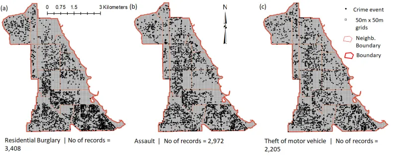
The study area selected for this research is the south side of Chicago, henceforth denoted as South Chicago. South Chicago measures approximately 12 km and 10 km North-South and East-West, respectively. The crime data set can be downloaded from the website www.cityofchicago.org. Three crime types that are potentially different in terms of the spatial and temporal characteristics are selected. They include: residential burglary (with 3,408 records), assault (with 2,972 records) and theft of motor vehicle (with 2,205 records) crimes between the period of1stMarch 2011 and8thJanuary 2011; the same data set used
in [1].
It is noted that the geo-coding of these open datasets have changed recently from snap-ping crime events to individual buildings, to resolving them to the (approximate) centre of each city block. The latter option, as currently available from the website, is used in this study.
Prior to any advanced analysis of a spatiotemporal data set, it is necessary to probe the spatial and/or temporal patterns of the data set, in order to gain a first-hand insight into the spatial and temporal characteristics that can help to explain subsequent results. This is often carried out through visual exploration. Thus, visualizations of the spatial distribution of the three crime types will first be provided in the next subsection. We chose to explore only the spatial patterns of the point datasets as they are more relevant to this work, and can provide rough pictures of the potential areas of hotspots. Following that, the parameter setting forKandT will be discussed and lastly, the details of the analyses.
3.1
Exploration of the spatial patterns of the data sets
The purpose of the exploration here is to gain insight into the spatial patterns of the three crime data sets through visual inspection. Figure 2 is the spatial point distribution of the data sets displayed on a grid system of 50m by 50m created over the study area; to also be used later for modelling the final hotspot map. This grid cell size of 50m x 50m has previously been used in Mohler et al. [17] and was also confirmed by Adepeju and Evans [2] to be very effective in capturing the RNRV of crime data sets of South Chicago area.
Figure 2 demonstrates that each crime type has a varied level of crime concentration across different regions of the South Chicago area. The burglary crime shows the densest concentration, especially within neighborhoods that are highly residential (south-eastern parts). The concentration level is lessened towards the northern part of the area. This is in contrast to both the assault and theft of motor vehicle data sets, which are both fairly dispersed across the entire area. In comparison to the theft of motor vehicle sets, the assault crime set demonstrates some clearly identifiable hotspot regions (Figure 2b), whereas the theft of motor vehicle crimes are spatially more dispersed across the area. For the three crime data sets, the events’ distribution can be said to reflect the land use pattern of the area. As an example, the central part of the area, where the University of Chicago is situated, shows little or no burglary crime; due to a lack of residential buildings. Furthermore, there are a very limited number of assault crimes within this area. On the other hand, there are many instances of theft of motor vehicles in this region.
Figure 2: Spatial patterns of the case data sets.
3.2
The values of the maximum spatial and temporal thresholds
(K and T)
The minimum value ofKto be used in this study is 50m. This is selected for two important reasons: one, to conform to the grid system created (i.e., 50m x 50m, see Section 3). If any two values ofKare smaller than the size of the grid cells, their results are highly likely to be very similar. That is due to the fact that many cylinder surfaces will fall completely inside the cells, and therefore will pick up the same grid cells (see Figure 1). Secondly, it can be observed from the spatial distribution of the data sets, especially the burglary and assault ones, that many events are repeated spatially within very close distances. Hence, a spatial radius distance of 50m will enclose a considerably larger number of events. Finally, the list of values forK created areK= [50m, 150m, 250m, 500m, 1000m, and 12×the size of the
study area].Half of the size of the study areais included as it constitutes the most commonly used value of K. It is calculated as: (North-South extent of the study area + East-West extent of the study area)/4. Based on the size of the South Chicago study area,half of the size of the studyarea is estimated to be 5.5km.
The minimum value ofT to be used is 14 days (2 weeks) in order allow weekly and fortnight cyclic patterns to be captured. It is obvious that different regions across the area may possess different temporal patterns. Therefore, a sufficiently large value ofT may be required in order for each region to be fitted with its appropriate temporal window size. The final list of values created forT isT = [14 days, 30 day, 60 days, 90 days, and 1
2×the
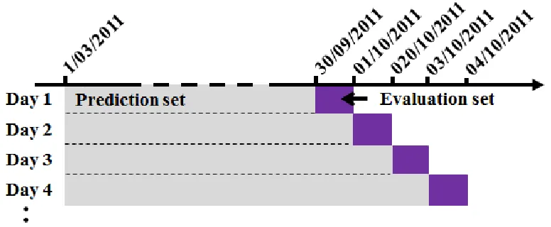
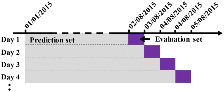
Figure 3: The predict-evaluate routine.
3.3
The training and evaluation process
The temporal range of each crime type is between1st March 2011 and8thJanuary 2012.
In this analysis, the first training set is from the1stMarch 2011 to30thSeptember 2011 (7
months). The training refers to the process of generating predictive hotspots as illustrated in Figure 1 (from the generation of cylinders to the hotspot surface modeling). The first evaluation (i.e., the calculation of the hit rate for the first hotspot surface) will be based on the next one-day dataset (i.e., the dataset of1st October 2011). Next, the second training
data set will combine the immediate previous evaluation dataset with the training data set to form the new training data set. In essence, the start date of all the training data sets will be fixed as1st March 2011, while the end dates will be made to increase by 1 day as the predict-evaluate routine progresses; for a given value of K being examined (see Figure 3). This process is repeated for 100 daily consecutive steps. The evaluation data length of 1-day is chosen to conform to the short-term operational practice for day-to-day crime prediction by many police agencies. For the purpose of this study, we employed thersatscan pack-age inRwhich allows the SaTScanTM software to be called fromRenvironment, thereby
facilitating automation and repeated analysis [13].
4
Results and discussion
The primary objective of this study is the development of an optimization strategy through which the impacts of the spatial and temporal thresholds of the PSTSS technique on the predictive accuracy can be investigated.
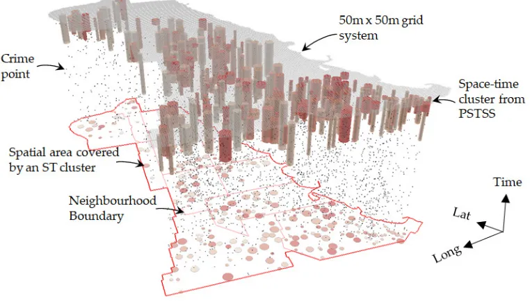
7thJanuary 2012, and the anticipated crimes are the next one-day’s worth of crime events (i.e., for8thJanuary 2012). The figure is for a spatial and temporal threshold of 150m and 60 days, respectively. The intensity of the cylinder, ranging from deep red to grey; repre-sents the riskiest and the least risky clusters, respectively. The concentration of the clusters reflects the spatial distribution of the crime events, as illustrated in Figure 2a. The distribu-tion of the riskiest clusters is irregular across the area.
Figure 4: A 3D visualization of the burglary clusters from the PSTSS for the100thpredictive
step (i.e., date: 7thJanuary, 2012) with the spatial and temporal thresholds of the scanning
window as 150m and 12×the length of the study period, respectively. The intensity of the
cylinders (ranging from grey color to deep red color) represent the risk level within each region. The base map shows the boundaries of the twelve neighborhoods of the South Chicago area.
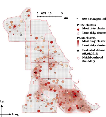
In practice, the use of prediction results is usually based on a 2D map representation. The 3D representation in Figure 4 can be transformed into a 2D map by overlaying the cho-sen grid system (i.e., 50m x 50m) on the generated clusters. Figure 5 is the corresponding 2D map of the 3D representation of Figure 4, based on the description in section 2.1. The 2D representation allows for the easy identification of location and makes the evaluation process much easier to carry out.
Figure 5: The corresponding 2D cluster map of the 3D results shown in Figure 4. The points (stars) are the evaluated data sets at the100thpredictive step. The continuous surface is the
top 20% risk locations generated by the PKDE method using the recent 90 days’ datasets. The clusters by both methods are resolved onto the 50m x 50m grid system in order to generate hotspot maps.
For both methods, the evaluation process is based on the ranking of the intersecting grid cells with the clusters, with clusters selected in the order of their intensity level. In the case of the PSTSS, the value of K andT strongly determines the amount of hotspot coverage that is generated. This is due to the fact that a much larger hotspot coverage is likely to be generated for large values ofKandT (e.g., 1000 m and 90 days, respectively) compared to small values ofKandT (e.g., 50 m and 14 days, respectively). The hotspot coverage is important to patrol teams, especially when there is limited amount of available resources.
In the figure, the overlayed points (i.e., the stars) are the anticipated crime events of the next one day (8thJanuary 2012). It can be seen that, while some events were exclusively
captured by each method (e.g., point 5 and point 4 for the PSTSS and PKDE, respectively), some were jointly captured by both methods (e.g., points 1, 2, 3, 6, and 7). It is also possible for both methods to miss a point entirely, such as point 8. In terms of the accuracy, these indicate a separate 12.5% hit rate by each method and a joint 62.5% hit rate by both meth-ods. The separate hit rates are largely due to the differences in the spatial distribution of the hotspots generated by the two methods.
By examining the accuracy of the hotspots at various coverages, a full understanding of the performance of each method can be gained. In order to simplify the results of different combinations ofKandT, it was decided to examine the accuracies (mean hit rate) at only five hotspot coverages between 0 to 20%, where applicable. The coverages identified were 1%, 5%, 10%, 15%, and 20%. In the additional analysis to demonstrate the distinctiveness of PSTSS as compared to the PKDE, all coverages from 1 to 20% were used.
4.1
Predictive accuracies of PSTSS at different spatial and temporal
thresholds
Based on the values of K and T created in Section 3.2, the mean hit rate of the PSTSS hotspot method is evaluated at different combinations ofKandT. The goal is to answer the question, "at what value ofK and/orT is the accuracy highest (or optimized)?" The mean hit rates at the selected coverages (1%, 5%, 10%, 15%, and 20%, where applicable) are calculated using Equation 3.
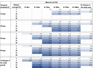
Table 1: The predictive accuracies of the PSTSS at various spatial and temporal thresholds for burglary crime. The gradient shades of blue highlight the relative accuracy of the cells assessed by hit rate.
The overall pattern of the mean hit rate, as shown in Table 1, is thatK impacts the accuracy more strongly thanT. Moreover, the mean hit rate decreases asKincreases from
K= 50 m toK=12×the size of the study area. In other words, the best predictive accuracy
is obtained atK= 50 m and the worst predictive accuracy is obtained atK= 12×the size
of the study area. This implies that the PSTSS is able to capture the RNRV pattern more effectively when scanning windows are more focussed on the small local neighborhood. Aside from the tendency to generate very low hotspot coverage at small values ofK, the accuracy produced is very impressive. For example, an accuracy produced at a hotspot coverage of 5% atK= 50 m (andT = 1
2×the length of study period) is 22.4%; which is a
19%, 76%, and 136% improvement over the corresponding accuracies atK = 150 m,K = 750 m andK= 1
2×the size of the study area, respectively.
to effectively capture all the necessary emerging clusters. However, any other values ofT
[image:15.612.115.514.150.450.2]from 30 days upward, in conjunction with itsKcounterparts, offers improved accuracy.
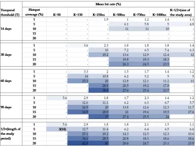
Table 2: The predictive accuracies of the PSTSS at various spatial and temporal thresholds for assault crime. The gradient shades of blue highlight the relative accuracy of the cells, as assessed by hit rate.
In Table 2, the results of the assault crime are shown. Similar patterns, in terms of the coverages and mean hit rates in relation to both spatial and temporal thresholds, can be ob-served. Much like in Table 1, most of the missing results are a result of insufficient clusters being generated due to small values ofKandT. Moreover, the mean hit rate increases as the value ofKdecreases. Across all values ofT, a similar mean hit rate is obtained at the same coverage level. In comparison with the results for burglary, a relatively lower mean hit rate is generated for each corresponding intersection ofKandT. This implies that there is a higher RNRV pattern in burglary crime compared with assault crime. Although, the difference in the levels of RNRV patterns in both crime types is apparent from Figure 2, though burglary crime shows a higher event concentration than assault crime. Burglary crime has 436 more crimes than assault, as well as a lower level of event dispersion.
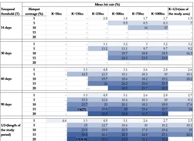
Table 3: The predictive accuracies of the PSTSS at various spatial and temporal thresholds for theft-of-motor vehicle crime. The gradient shades of blue highlight the relative accuracy of the cells as assessed by the hit rate.
KandT, and patterns of the mean hit rate as their values, especially in relation to that of
Kchanges. In comparison with burglary and assault crimes, the general accuracy level of the theft of motor vehicle crimes is lower. This is attributed to the higher level of spatial dispersion of the data set compared to burglary or assault crime.
In summary, these results show that the spatial threshold (K) of the scanning window is a more influential parameter on the accuracy of the PSTSS than the temporal threshold (T). Particularly, whenK= 50 m, which is equivalent to the adopted grid system cell size, the accuracy is highest. At larger values ofK andT, however, a larger hotspot coverage level (up to 20%) is possible, which is sufficient for many practical applications; the main limitation being a relatively lower level of accuracy. In other words, the accuracy may not be optimal when a large hotspot coverage is generated.
4.2
Validation of the results
Therefore, the same analysis was repeated using datasets spanning a different time period, between 1st January 2015 and 10th November 2015. The same crime types were main-tained: residential burglary, assault, and theft of motor vehicle. The datasets here appear to be lower in terms of the number of records by 47%, 24% and 48%, respectively. The same parameter values forKandT; that isK= [50m, 150m, 250m, 500m, 1000m, and1
2×the size
of the study area], andT = [14 days, 30 day, 60 days, 90 days, and 12×length of the study period] are utilized. Moreover, the samepredict-evaluateroutine strategy was employed, as described in Figure 3. In this case, the first prediction set is now the datasets between1st
January 2015 and2ndAugust 2015, while the first evaluation set is the dataset of the next
one day, which is the3rdAugust 2015. Thepredict-evaluateroutine was then continued for
the next 99 days. The full details of the results of this validation exercise can be found in the supplementary document of this article.
In summary, the results of the validation exercise support the patterns of results ob-tained in the Tables 1, 2, and 3. That is, it was found that the three key observations were true: (1) that the hotspot coverage increases as the values ofK and T increase, (2) that
Kshows more influence on the mean hit rate thanT, with mean hit rate decreasing asK
increases, and (3) that a trade-off exists between the hotspot coverage and the mean hit rate; except for the hotspot coverage obtained whenK= 1
2×the size of the study area.
4.3
Distinctiveness of the predictive capabilities of PSTSS method
In Figure 5, the distinction between the spatial distribution of the hotspots generated in the first test by both the PSTSS and the PKDE were visualized. The hotspots by the PSTSS are a set of irregularly distributed circles across the study area, argued to reflect the dynamics of the most recent events across the area. This, therefore, suggests that the PSTSS is likely to capture some crimes that are distinct from the crimes that would be captured by a method such as the PKDE. In order to test this hypothesis, it was decided that a scenario whereby both the PSTSS and the PKDE generate the same mean hit rate needed to be examined to determine how the actual crimes captured by both methods are the same or different.
Following thepredict-evaluate routine illustrated by Figure 3, we then used the PKDE to also predict the three crime types, following the predict-evaluateroutine, as illustrated by Figure 3. However, instead of using a fixed start date for all the predictions, a rolling 90-day time window was employed, which ensures that the start date is moved forward by the predictive step (i.e., one day) as the predictions progress. By using a rolling 90-day window for the training/prediction, it is assumed that the 90 days historical events are a good predictor of the next one-day’s worth of crimes.
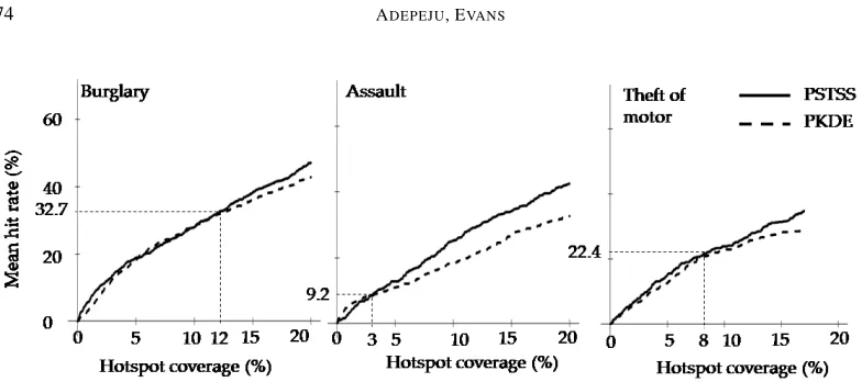
Figure 6 is the hit rate plot comparing the accuracies of the PSTSS and PKDE for all coverages between 0 and 20% for burglary and assault crimes, and between 0 and 17% for theft of motor vehicle crimes. Again, 17% is the maximum hotspot coverage attained by the PSTSS for the theft of motor vehicle data at the chosen spatial and temporal thresholds. The results of the PSTSS shown in the plot is based on the results generated for K=150 m andT =1
2×the length of study period (see Tables 1, 2, and 3).
Figure 6: Comparison of the accuracies of the PSTSS and PKDE methods.
[image:18.612.105.495.381.551.2]spatial distribution of the hotspots. It is argued that the revelation of these differences will not only help to show the distinctiveness of the PSTSS as compared to the PKDE, but may help in understanding the predictive capabilities of the former, and open up opportunities for improvement.
Figure 7: Venn diagram showing the accuracy statistics of the PSTSS and PKDE at the 12% and 8% hotspot coverages for the burglary and theft of motor vehicle crimes, respectively. The percentage values in brackets represent the mean hit rate at the specified coverage over the prediction period. The shaded areas indicate the proportion of crimes captured exclusively by each method.
theft of motor vehicle crimes, respectively. From the Venn diagram, it can be observed that while both methods captured some of the exact same future crimes (represented by the intersection area), each individual method is also able to capture a significant proportion of other future crimes. For example, in Figure 7(b), the proportion of crimes captured by each method (89 crimes≡14.9%) doubles the proportion that is jointly captured by both methods. These results support the observation in Figure 5 which suggests that the PSTSS and KDE may have different capabilities, in terms of the nature of future crimes that they capture.
The above exploration demonstrates that not only is the PSTSS able to produce a relat-able level of accuracy, but is also relat-able to predict some distinct crimes that are not captured by a conventional hotspot method, such as the PKDE. It is argued however, that there is a need for further investigation of these patterns in order to fully understand the underlying variables that influence the performance of the PSTSS, as well as the key characteristics of the crimes captured by the method.
5
Conclusion and future work
The PSTSS, a geographical surveillance technique, was used here as a hotspot method for short-term crime prediction. First, this study aimed to provide more technical informa-tion regarding the implementainforma-tion of the PSTSS hotspot technique, the details of which are missing in previous studies. The purpose of this study was to determine the optimal values of the spatial and temporal thresholds by which the predictive accuracy could be maximized. The significance of this study is that the optimization approach proposed here is not only usable for crime predictions, but is also applicable to other areas, such as pub-lic health and epidemiology, where the PSTSS is already widely used. Since the primary goal of this study was to determine the optimal values of spatial threshold (K) and tem-poral threshold (T) that maximize predictive accuracy, a list of the values ofKandT were created, which included small, medium, and large values. This allowed for the testing of different ideas proposed in previous studies regarding the size ofKandT. The choice of
K andT is relevant in crime data analysis as it allows for different sizes of geographical neighborhood to be properly examined in relation to crime risk.
In order to evaluate the performance of PSTSS as the valuesKandT change, we con-sidered a real-life operational uptake of the method. The patrol officers want to be able to intersect as many crimes as possible with a limited patrol coverage. Therefore, we used the metric called hit rate (equation 2, [5]) which quantifies the proportion of crimes that would potentially be intersected if the officers focus on a specified hotspot coverage. In other words, the use of hit rate as an evaluation criterion provides operational advantage over the derived likelihood ratio in equation 1 which has a limited operational relevance.
For the prediction results across the three crime types, two features were prominent. First, was the pattern of the mean hit rate and second, was the pattern of the hotspot cov-erage. Incidentally, these constitute two important factors when choosing between various existing predictive hotspot methods. They are categorized in terms of predictive accuracy and usability, respectively. In choosing a predictive method, an enforcement agent wants to ensure that the method is as accurate as possible and further, that the method is usable in terms of generating sufficient hotspot coverage at all times. There is a strong relation ob-served between these two factors as the values ofKandT are varied. The general pattern is that where the technique has the tendency to generate highest accuracy, the coverage level is minimal. These are specific to small values ofKandT. For example, atK= 50 m andT= 30 m, no hotspot is reported. Whereas better coverage is gained as these values are increased, but this is also accompanied by a decrease in the level of accuracy. Generally, a sufficient amount of hotspot coverage, such as 15%, is consistent for the crime types at the
KandT values of 150 m and 90 days, respectively.
Interestingly however, theK andT impacts upon the accuracy level very differently. For instance,K is observed to be the major influence on the accuracy obtained while the impact ofT is very negligible. AsK increases, the accuracy level decreases. Therefore, the worst accuracy level is attained atKequals half of the size of the study area—a value which has been widely used in many other studies. The only impact ofT on the accuracy is seen at T = 14 days, where it is worst. The accuracy is generally stable fromT = 30 days upwards. While previous suggestions regarding the choice ofK and T may work adequately for other applications, the results in this study suggest that those suggestions are applicable predictive hotspot of short-term crime hotspot prediction. Furthermore, we included a validation study that showed that we can generalize the results obtained in this study for the selected crime types for the South Chicago area.
In summary, this study has demonstrated an optimization approach through which the best values of spatial and temporal threshold of the PSTSS hotspot technique can be de-termined in order to maximize accuracy of crime prediction. The primary key is to first determine the objective function to be maximized or minimized and systematically select values of the parameters to be optimized. While this approach is demonstrated for crime hotspot prediction, it is argued that it may be applicable to other similar studies in the pub-lic health and epidemiological domains. Furthermore, while the absolute figures derived in this study relate to the variations in space and time of Chicago and its crimes, the overall trends are likely, if not absolutely likely, to be similar across other cities.
It is important to mention that the grid-based version of the PSTSS that uses the Eu-clidean distances is employed in our study. A network-based variant that is based on street network distances has been implemented in [20] and used for crime prediction. The im-plementation of network-based PSTSS is beyond the scope of this study. However, we also intend to implement the network-based method in the future and compare their perfor-mances.
datasets. Thus, the examination of such responses in relation to the PSTSS will be the subject of future investigation.
Acknowledgments
This work was funded by the UK Home Office Police Innovation Fund, through the project “More with Less: Authentic Implementation of Evidence-Based Predictive Patrol Plans.”
The authors would like to acknowledge the contribution of the UCL Crime, Policing and Citizenship project supported by UK EPSRC (EP/J004197/1), as well as the principal inspector of the project, Prof. Tao Cheng.
The authors also want to acknowledge the contribution of Dr. Matthew Daws for pro-viding insightful comments on the original version of this paper.
References
[1] ADEPEJU, M., ANDCHENG, T. Determining the optimal spatial scan of prospective space-time scan statistics (PSTSS) for crime hotspot prediction. In25th GIS Research UK Conference(2017).
[2] ADEPEJU, M.,AND EVANS, A. Investigating the impacts of training data set length (t) and the aggregation unit size (m) on the accuracy of the self-exciting point process (SEPP) hotspot method. In2017 International Conference on GeoComputation.(2017).
[3] ADEPEJU, M., ROSSER, G., AND CHENG, T. Novel evaluation metrics for sparse spatio – temporal point process hotspot predictions – a crime case study. International Journal of Geographical Information Science 30, 11 (2016), 2133–2154. doi:10.1080/13658816.2016.1159684.
[4] BOWERS, K., AND JOHNSON, S. Domestic burglary repeats and space-time clus-ters: The dimensions of risk. European Journal of Criminology 2, 1 (2005), 67–92. doi:10.1177/1477370805048631.
[5] BOWERS, K., JOHNSON, S., AND PEASE, K. Prospective hot-spotting: The fu-ture of crime mapping? British Journal of Criminology 44, 5 (2004), 641–658. doi:10.1093/bjc/azh036.
[6] CHAINEY, S., TOMPSON, L., AND UHLIG, S. The utility of hotspot mapping for predicting spatial patterns of crime. Security journal 21, 1–2 (2008), 4–28. doi:10.1057/palgrave.sj.8350066.
[7] CHEN, H., CHENG, T., AND WISE, S. Developing an online cooperative police pa-trol routing strategy. Computers, Environment and Urban Systems 62 (2017), 19–29. doi:10.1016/j.compenvurbsys.2016.10.013.
[9] COSTA, M., KULLDORFF, M., AND ASSUNÇÃO, R. M. A space time permutation scan statistic with irregular shape for disease outbreak detection. Advances in Disease Surveillance 4(2007), 243.
[10] DUONG, T.,ANDHAZELTON, M. Cross-validation bandwidth matrices for multivari-ate kernel density estimation. Scandinavian Journal of Statistics 32, 3 (2005), 485–506. doi:10.1111/j.1467-9469.2005.00445.x.
[11] ECK, J., CHAINEY, S., CAMERON, J., LEITNER, M.,ANDWILSON, R. Mapping crime: Understanding hot spots. Tech. rep., National Institute of Justice, Washington, DC, 2005.
[12] FARREL, G.,ANDPEASE, K. Once bitten, twice bitten: Repeat victimisation and its impli-cations for crime prevention. Crown Copyright, 1993.
[13] KLEINMAN, K. rsatscan: Tools, classes, and methods for interfacing with SaTScan stand-alone software. R package, version 0.3, 9200. Tech. rep., 2015.
[14] KULLDORFF, M. Software for the spatial and space-time scan statistics. SaTScanTM
version 7.0. Tech. rep., Information Management Services, Inc., 2006.
[15] KULLDORFF, M., HEFFERNAN, R., HARTMAN, J., ASSUNÇÃO, RENATO, M., AND MOSTASHARI, F. A space time permutation scan statistic for disease outbreak detec-tion.PLoS Medicine 2, 3 (2005), e59. doi:10.1371/journal.pmed.0020059.
[16] LEITNER, M., AND HELBICH, M. The impact of hurricanes on crime: a spatio-temporal analysis in the city of houston, texas. Cartography and Geographic Information Science 38, 2 (2011), 213–221. doi:10.1559/15230406382213.
[17] MOHLER, G., SHORT, M., BRANTINGHAM, J., SCHOENBERG, F. P.,AND TITA, G. E. Self-exciting point process modelling of crime. Journal of the American Statistical Asso-ciation 106, 493 (2011), 100–108. doi:10.1198/jasa.2011.ap09546.
[18] NAKAYA, T., AND YANO, K. Visualising crime clusters in a space-time cube: An exploratory data-analysis approach using space-time kernel density estimation and scan statistics. Transactions in GIS 14, 3 (2010), 223–239. doi:10.1111/j.1467-9671.2010.01194.x.
[19] NEILL, D. Detection of spatial and spatio-temporal clusters. PhD thesis, Carnegie Mellon University, 2006.
[20] SHIODE, S., ANDSHIODE, N. Network-based space-time search-window technique for hotspot detection of street-level crime incidents.International Journal of Geographical Information Science 27, 5 (2013), 866–882. doi:10.1080/13658816.2012.724175.
A
Appendix: Validation study
A.1
Aim
To examine whether the PSTSS (parameter sweep) results shown in the Tables 1, 2, and 3 of the main manuscript can be generalised for the South Chicago. The following are the three key patterns observed when the values of the parameters K (the spatial threshold) and T (the temporal threshold) are varied:
1. The hotspot coverage increases as the values of K and T increase.
2. K shows more influence on the mean hit rate than T. As K increases, the mean hit rate decreases.
3. A trade-off exists between the hotspot coverage and the mean hit rate; except for the hotspot coverage obtained when K =12 of the size of the study area.
Goal of the validation study:
To test whether the above three patterns will be observed for another dataset (of the South Chicago area) covering a different period.
A.2
Data sets, parameter settings, and procedures
Datasets:
In order to carry out this validation study, the South Chicago crime datasets (from www.data.cityofchicago.org) were downloaded for a different time period. That is, from 1st January 2015 to 10th November 2015, as opposed to the period 1st March 2011 to 8th January 2012, which was used in the main analysis. It was ensured that both datasets were of the same length in terms of the number of days. The same crime types were also maintained, namely: residential burglary, assault, and theft of motor vehicles. The datasets have 1,821 records, 2,253 records and 1,146 records, respectively. Compared to the ones used in the main manuscript, the number of records in these datasets are lower by the percentages of 47%, 24% and 48%, respectively. As a result, the spatial point distributions appear relatively sparser, as shown in Figure A1 when compared with Figure 2 of the main manuscript.
Parameter settings:
The same parameter settings used in the main manuscript for both K and T were main-tained. They are:
• K = [50m, 150m, 250m, 500m, 1000m, and12 of the size of the study area] • T = [14 days, 30 days, 60 days, 90 days, and12of length of the study period]
Procedure:
Figure A1: Spatial point distribution of the validation datasets.
August 2015, which is evaluated against the next one-day dataset (i.e. 3rd August 2015). The predict-evaluate process is continued by incrementing the prediction set by one day and evaluating against the next one-day dataset until the 10th November 2015. This makes a total of 100 “predict-evaluate” steps.
Figure A2: Predict-evaluate routine for the validation study.
A.3
Results
Predictive accuracies of PSTSS at different spatial and temporal thresholds:
[image:24.612.107.490.397.554.2]5%, 10%, 15%, and 20% (where applicable). These are shown in Tables A1, A2, and A3. The gradient shades of blue colour are also applied to the cell values in order to highlight their relative magnitude.
[image:25.612.113.512.198.495.2]Tables A1, A2, and A3 represent the results for burglary crime, assault and theft of motor vehicle crimes, respectively. These tables will now be discussed in terms of the patterns of their coverages (missing values) and the predictive accuracies.
Table A1: The predictive accuracies of the PSTSS (for the validation dataset) at various spatial and temporal thresholds for burglary crime.
Hotspot coverages (and missing values):
Table A2: The predictive accuracies of the PSTSS (for the validation dataset) at various spatial and temporal thresholds for assault crime.
slightly more cells with missing values in the validation results as compared to the main results. This can be attributed to the relative sparsity of the validation datasets as compared to that of the main dataset. In conclusion, the patterns of the hotspot coverages or missing values in this validation exercise correspond with those in the main manuscript.
Patterns of the mean hit rates:
Similar to the pattern of the mean hit rates obtained in Tables 1, 2, and 3 of the main manuscript, K appears to impact upon the accuracy more strongly than T. The mean hit rate decreases as K increases from K = 50 m to K =1
2of the size of the study area, for almost
all values of T. Thus, the best predictive accuracy is obtained at K=50 m and the worst predictive accuracy is obtained at K =1
2 the size of the study area. The lack of many values
Table A3: The predictive accuracies of the PSTSS (for the validation dataset) at various spatial and temporal thresholds for theft-of-motor vehicle crime.
dataset for the prediction may help to improve the number of entries in the K=50m column, thereby allowing the best values of the mean hit rate to be obtained at K=50m.
Demonstrating similar patterns as in the main manuscript, the temporal threshold, T, showed little or no impacts on the mean hit rate. There are no significant increases or decreases in the mean hit rate across all values of T at each corresponding coverage level.
A.4
Conclusion
The goal of this validation study is to examine whether the pattern of the accuracies and the coverages generated when the parameters K and T of the PSTSS hotspot method are var-ied during the prediction of South Chicago’s crime datasets can be generalised. A similar analysis was then performed on datasets of a different study period (between 1st January 2015 and 10th November 2015), experimenting with the same parameter settings for the K and T.
(3) that a trade-off exists between the hotspot coverage and the mean hit rate except for the hotspot coverage obtained when K =1
2 of the size of the study area.