Surface wave studies of the Australian upper mantle

AUSTRALIAN UPPER MANTLE

A thesis submitted for the

degree of

DOCTOR OF PHILOSOPHY

in the

Australian National University

by

JOHN HENRY GONCZ

Frontispiece

F

r

e

q

u

e

n

c

y

-t

i

m

e

a

n

a

l

y

s

i

s

o

f

summed

c

r

o

s

s

-c

o

r

r

e

l

a

t

i

o

n

s

—

grou

p

ve

loc

STATEMENT

The studies described in this thesis were carried out while I was a full-time research scholar at the Australian National University, Canberra, A.C.T.

Except where mentioned in the text or in the preface, the research described in this thesis is my own.

This thesis has never been submitted to another university or similar institution.

ABSTRACT

The analysis and inversion of Australian surface wave data

indicates the presence of a well-defined low shear velocity channel in the upper mantle under eastern Australia between depths of 90 and 200 km, and the absence of a similar structure beneath the shield area of central and western Australia.

Frequency-time analysis of the sum of cross-correlations of many surface wave records made possible the determination of Rayleigh wave group velocities over the extremely wide period range 10 to 180 s.

Smooth Rayleigh wave phase velocity curves have been obtained by

integrating the group velocity curves. Since no other filtering is used in processing the data, these results constitute unbiased dispersion observations. Monte Carlo inversion of these data shows that accurate group velocity measurements are needed to reduce the non-uniqueness

bounds of Earth models. There is an anomalous, and perhaps questionable, dip in the group velocity curve at around 110 s for some of the eastern paths. It is not apparent in western Australia. Love wave group

velocity measurements are perturbed by interference between the fundamental mode and higher modes. Nevertheless, Love wave phase velocities have been measured with sufficient accuracy by averaging an ensemble of events with varying epicentral distances. Low contrast models of the crust and upper mantle which fit the Rayleigh wave

observations do not fit the Love wave data. The fitting problem is more pronounced in eastern Australia. Inclusion of a thin almost-liquid layer into the models enables a better fit to both Rayleigh and Love wave

PREFACE

The Earth’s upper mantle has become an increasingly active area of geophysical research, largely because more precise information about the characteristics of the low velocity zone which it contains is vital to the understanding of the mechanics of plate movements. The theory is widely accepted that material within the low velocity zone is partially melted and acts as a lubricant upon which the plates can slide, as well as providing the return path in the advective/convective cycle.

Information about the low velocity zone can be obtained from body wave observations and also from geochemical information derived from

laboratory experiments, but analysis of surface wave dispersion provides the most definitive information about shear wave velocities in the region, and these in turn can supply the most direct evidence of partial melting.

The presence of noise complicates the analysis and interpretation of surface wave data, by reducing the precision of

velocity measurements and by restricting the range of periods that can be analysed. On the other hand, theory and experience both show that high- precision dispersion information over an extended period range is needed to delineate the structure of the upper mantle. Diverse methods for overcoming these problems have been proposed. The method of summing cross-correlations of signals from events at varying epicentral distances, which forms the basis of the present study, is in many respects analogous to techniques in seismic array processing which have resulted in an order of magnitude enhancement of body wave signals.

The project of studying the upper mantle under the Australian continent was initiated in April 1972 by Dr John Cleary's suggestion that the results of a Rayleigh wave study of this region by Thomas [1968] might be extended by the use of now available, more powerful methods of surface wave analysis.

used in the course of his investigations. The major ones are:

Dr A. Dziewonski GROUVE (multiple filter analysis)

Dr R. Masse TEQUILA (surface wave computation)

Mr J.A.B. Palmer LIN36 (contouring program).

GROUVE had to be completely rewritten in order to fit on a mini-computer, and this exercise afforded a thorough understanding of its capabilities. Several other programs, such as distance and azimuth computation, have been used. Originating from various sources, these programs are now part of the library of any geophysical research establishment.

The major geophysical contributions arriving from this study are listed below. Contributions to information science are also included in the list.

1. The existence of a well-defined low shear velocity channel in the upper mantle under eastern Australia, in the depth range 90 to 200 km, has been established.

2. The upper mantle under central and western Australia does not contain a similarly well-defined low velocity channel. In this respect it is similar to shield areas found in other parts of the world. The difficulty which this observation presents to the theory of plate tectonics does not appear to be generally recognized.

3. Group velocity measurements of surface waves with periods from 10 s to 180 s have been obtained for well-defined geological regions by the combined use of sums of cross-correlations and addition of their frequency-time analysis matrices. This is a major extension of the period range usually encompassed by group velocity studies, and has made possible the advances in surface wave observation and analysis indicated below.

4. Smooth phase velocity curves have been obtained by integration of the group velocity curves. Since this process incorporates

information into the phase velocity curve additional to that obtained by harmonic analysis alone, it is superior to conventional smoothing

techniques.

of the Earth and found to be concordant. This has not been accomplished prior to this study.

6. The Australian surface wave observations confirm the difficulty of fitting Rayleigh and Love wave data simultaneously to isotropic Earth models, especially for continental-tectonic paths. Although this problem is not solved, application of the work of others shows that special

models which include anisotropic conditions or thin high-contrast layers can satisfy the data.

7. The upper mantle models derived by the present study are in harmony with other geophysical observations in Australia. They are, however, in apparent conflict with observations of P and S station

anomalies from which the presence of partial melting in the upper mantle was originally inferred. This may indicate the need for more

sophisticated modelling techniques in which, perhaps, the effects of lateral heterogeneity need to be explored.

8. Mode interference of Love waves has been demonstrated with real data, showing that group velocity measurements are perturbed, and

consequently that the determination of phase velocities obtained by integration of group velocities is unreliable for Love waves.

Nevertheless, sufficiently accurate measurements of Love wave phase velocities have been obtained by Fourier analysis of sums of cross­ correlations of ensembles of signals from events at varying epicentral distances.

9. A novel, efficient, accurate computer-assisted digitizing system has been devised.

10. A major surface wave study has been implemented on a mini­ computer.

11. Automated methods of handling seismic information have been

developed using state-of-the-art computer programs and peripheral devices. Contour plots of frequency-time analyses of signals were found to be a form of graphic output capable of presenting large amounts of information in a manner suitable for human assimilation and evaluation. It is

ACKNOWLEDGEMENTS

Dr R.S. Anderssen helped formulate the approach used in the Monte Carlo inversion of the data. The ANU Computer Centre*s UNIVAC 1108 computer was used to perform the inversion, and it is a pleasure to

acknowledge the support of the staff of the Centre.

Professor Anton L. Hales, Director of the newly-established Research School of Earth Sciences,gave the author considerable guidance and stimulation stemming from his extensive experience in geophysics.

Members of the Department of Engineering Physics, Messrs J.W. Blarney and C.W. Vance afforded many worthwhile discussions. Dr I.D.G. McLeod is especially thanked for his computing advice. He was also responsible for the superlative PDP-15 computing installation used for the major part of this study. The use of the facilities of the

department, headed by Professor S. Kaneff, is gratefully acknowledged.

The friendship and interest of fellow research scholars,

Dr D.W. King and Dr M.H. Worthington, was apparent in their participation in many fruitful discussions.

Dr Cleary's long association with Australian geophysics was of great assistance in the interpretation of the inversion results within that framework, and his contribution is gratefully acknowledged.

I am sincerely grateful to my supervisors, Dr K.J. Muirhead and Dr Cleary, for encouragement and guidance throughout the study.

PUBLICATIONS

The papers listed below have resulted from the work described herein. A list of the author's previous publications, not related to the present study, is included in Appendix C.

J.H. Goncz (1972). - 'Computer aided digitization of seismic traces', Proceedings of the Decus-Australia August 1972 Symposium, pp.45-46. (abstract)

J.H. Goncz (1973). - 'Digital analysis of dispersed seismic signals', presented at first seminar on Digital Signal

J.H. Goncz (1974). - 'Computer aided digitization of chart records', J. Phys. E: Sei. Instrum. 7_, 20-22.

J.H. Goncz and A.L. Hales. - 'Analysis to extended periods of Rayleigh and Love wave dispersion across Australia'

(forthcoming).

J.H. Goncz, J.R. Cleary and K.J. Muirhead. - 'Variations in upper mantle structure beneath Australia from surface wave

C O N T E N T S

PREFACE v

CHAPTER 1. A REVIEW 1

1.1 Surface wave observations 1

1.2 Analytical methods for obtaining phase and

group velocity 4

1.3 Inversion 8

1.4 The present study 10

CHAPTER 2. DATA ACQUISITION AND DIGITIZATION 14

2.1 Data selection and acquisition 14

2.2 Digitization and management of data 21

2.3 Digitizing instruments 22

2.4 Digitizing system 24

CHAPTER 3. NUMERICAL ANALYSIS OF DISPERSED SEISMIC SIGNALS 28

3.1 Introduction 28

3.2 Phase velocity and group velocity 29

3.3 The two-station method 33

3.4 Time-varying filtration (TVF) 36

3.5 Cross-correlation 40

3.6 Frequency-time analysis (FTAN) 42

CHAPTER 4. ANALYSIS OF OBSERVED DISPERSION 47

4.1 Introduction 47

4.2 The path CTA-ADE: Rayleigh waves 48

4.3 Other Australian paths: Rayleigh waves 63

4.4 Further signal averaging 73

4.5 Derivation of phase velocity curves by integrating

group velocity 83

4.6 Discussion: Results at long periods 86

CHAPTER 5. INVERSION 111

5.1 The working model 111

5.2 Testing procedure 114

5.3 High contrast models 122

5.4 Higher Love modes 123

5.5 Conclusions 124

CHAPTER 6. DISCUSSION OF RESULTS 127

6.1 Comparison with other surface wave studies 128

6.2 Comparison with Australian body wave studies 132

6.3 Relation to other Australian geophysical data 137

6.4 Discussion: Anisotropy 138

6.5 A suggestion for further work 140

APPENDIX A. OBSERVED DISPERSION DATA 142

APPENDIX B. MONTE CARLO MODELS 144

APPENDIX C. PRIOR PUBLICATIONS BY AUTHOR 147

APPENDIX D. EXAMPLES OF SEISMIC DATA PRESENTATION 149

I L L U S T R A T I O N S

1.1 Knopoff’s phase velocity groups 5

2.1 Two-station sketch 15

2.2 Errors caused by great circle deviation 16

2.3 World map showing epicenters 17

2.4 Axes of some recording instruments 23

2.5 Computing loop used in digitizing seismograms 25

2.6 Digitizing with a Calcomp plotter (photo) 26

3.1 Phase velocity curves ADE-MUN 35

3.2 Group arrival event 3 at ADE:- (FTAN, TVF) 37

3.3 Group arrival event 3 at MUN:- (FTAN, TVF) 38

3.4 Group velocity FTAN plot of event 3 45

3.5 Flow chart of group velocity-FTAN-procedure 46

4.1 Group arrival event 7 49

4.2 Group arrival event 9 50

4.3 Group arrival event 12 51

4.4 Group arrival event 19 52

4.5 Group arrival event 21 53

4.6 Group arrival event 136 54

4.7 Phase velocity CTA-ADE (TVF) 55

4.8 Group velocity events 7, 9 57

4.9 Group velocity events 12, 19 58

4.10 Group velocity events 21, 136 59

4.11 Group velocity, sum of cross-correlations, CTA-ADE 60

4.12 Phase velocity CTA-ADE, comparison 61

Vector addition of signals and noise 63

4.13 Group velocity ADE-MUN, CTA-MUN:- (FTAN plot) 64

4.14 Group velocity CTA-TAU, ADE-TAU:- (FTAN plot) 65

4.15 Group velocity ADE-RIV, CTA-RIV:- (FTAN plot) 66

4.16 Group velocity RIV-MUN, RIV-TAU:- (FTAN plot) 67

4.17 Phase velocity for 9 paths, common scale 68

4.18 Phase velocity for 9 paths, displaced scale 69

4.20 Thomas's results for CTA-MUN, CTA-ADK /?

4.21 Knopoff, shield phase velocity curves 74

4.22 Knopoff, 'aseismic platform' phase velocity curves 75

4.23 FTAN plot ridge crests, all nine paths 76

4.24 'WA2' sum of FTAN matrices, Rayleigh wave 77

4.25a 'EA1' sum of FTAN matrices, Rayleigh wave 78

4.25b 'EA2' sum of FTAN matrices, Rayleigh wave 79

4.26 'Total' Australia sum of all FTAN matrices, Rayleigh wave 80

4.27 Rayleigh wave group velocity on linear period axis 81

4.28a 'WA2' family of phase velocity curves 85

4.28b 'EA2' family of phase velocity curves 86

4.29 Rayleigh wave phase velocity curves for Australia 87

4.30 Love wave group arrival, event 9 92

4.31 Love wave group arrival, event 21 93

4.32 Love wave group arrival, event 136 94

4.33 Love wave group velocity, events 9, 21 95

4.34 Love wave group velocity, event 136 96

4.35 Love wave group velocity, path RIV-MUN 97

4.36 Love wave group velocity, paths CTA-MUN, ADE-MUN 98

4.37 Love wave group velocity, paths RIV-ADE, RIV-TAU 99

4.38 Love wave group velocity, paths CTA-TAU, CTA-ADE 100

4.39 Love wave group velocity, paths CTA-RIV, ADE-TAÜ 101

4.40 'West' Australia Love wave group velocity:- (FTAN plot) 102

4.41 'East' Australia Love wave group velocity:- (FTAN plot) 103

4.42 'Total' Australia Love wave group velocity:- (FTAN plot) 104

4.43 Love wave group velocity in Australia 105

4.44a Love wave phase velocities for 9 paths, common scale 106

4.44b Love wave phase velocities for 9 paths, displaces axes 107

4.45 Love wave phase velocities, integrated group velocity

curves 108

4.46 'East' family of Love wave phase velocity curves 109

4.47 Partial derivatives from Bloch's model 110

5.1 'East' Monte Carlo models 116

5.2 Observed and calculated dispersion (Rayleigh, 'East') 117

5.3 Observed and calculated dispersion (Love, 'East') 118

5.4 'West' Monte Carlo models 119

5.5 Observed and calculated dispersion (Rayleigh, 'West') 120

6.1 Models from Knopoff [1972] 128

6.2 Comparison with shield models 130

6.3 Comparison with tectonic models 131

6.4 More 'East' Monte Carlo models 136

T A B L E S

2.1 Earthquakes used in this study 18

2.2 Characteristics of recording instruments 23

4.1 Event data for CTA-ADE path 48

A REVIEW

Lateral variation in the upper mantle beneath Australia has been suggested by heat flow studies and body wave information (discussed in detail in Chapter 6). The velocity and density structure of the Earth's upper mantle can be investigated by analysing the dispersion of surface waves that traverse a region and by inverting this information to find possible Earth models, the calculated dispersion of which matches the observed dispersion. Much progress has been made during the past decade in reducing the effect of noise always present in the observed data and in understanding what kind of information is needed to constrain possible Earth models in the inverse problem.

This dissertation studies the surface wave dispersion across the Australian continent and presents Earth models derived by inverting the information so obtained.

It will be shown that prior to this study the knowledge of surface wave dispersion across Australia was quite limited, and thus the first part of the study is acquisition of data. Secondly, the analysis

of dispersion is complicated by noise which limits the accuracy obtain­

able and the period range over which measurements can be made. Thirdly, the ultimate goal of inversion is to be able to make definitive

statements consistent with the observed data about the structure of the Earth in the regions concerned. This first chapter presents a review of major developments according to these three topics, and discusses their relevance to the thesis.

1.1 SURFACE WAVE OBSERVATIONS

as d i s t a n c e f r o m the s ource increases.

It is c o nvenient to c o n s i d e r s u r f a c e w a v e o b s e r v a t i o n s in three

c a t e g o r i e s :

(1) single o b s e r v a t i o n s f r o m a so u r c e d i r e c t to r e c o r d i n g

station, w h i c h can be called 'direct o b s e r v a t i o n s ' ,

(2) o b s e r v a t i o n s of the s ame w a v e t r a i n at two s t a t i o n s lying

on a great c ircle w i t h the l o c a t i o n of the e p i c e n t e r — the 'two-

s t a t i o n m e t h o d ' — and

(3) m u l t i p l e o b s e r v a t i o n s at the same s t a t i o n of a wave train

w h o s e a m p l i t u d e is large e n o u g h for it to b e d e t e c t e d a fter s everal

w o r l d - c i r c l i n g traverses.

D i r e c t o b s e r v a t i o n s and t w o - s t a t i o n o b s e r v a t i o n s a re u s e f u l in

s t u d y i n g the d i s p e r s i o n of limited, w e l l - d e f i n e d p o r t i o n s of the Earth.

M u l t i p l e o b s e r v a t i o n s of w o r l d - c i r c l i n g w a v e s c o n t a i n i n f o r m a t i o n o n l y

about the a v e r a g e p r o p e r t i e s of the E a r t h o v e r the great c i r c l e p ath

d e f i n e d by the loca t i o n s of the e p i c e n t e r and the r e c o r d i n g station. The

p r e v a l e n t m e t h o d of r e c o r d i n g a full d a y ' s d a t a as a h e l i c a l trace on a

r e v o l v i n g d r u m tends to m a k e di r e c t o b s e r v a t i o n of la r g e e a r t h q u a k e s

impossible. W h e n a la r g e amount of e n e r g y is r e l e a s e d at the s ource the

g a l v a n o m e t e r t race is either d r i v e n o f f - s c a l e or so s e r i o u s l y o v e r w r i t t e n

that the s e i s m o g r a m is indecipherable.

L o w a t t e n u a t i o n of the longer p e r i o d m a n t l e - s e n s i n g w a v e s

per m i t s o b s e r v a t i o n of m u l t i p l e c i r c u m f e r e n t i a l t r a v e r s e s a l ong time

after the earthquake, in some cases for days after. In o t h e r words,

direct o b s e r v a t i o n s are c h a r a c t e r i z e d b y r e l a t i v e l y h i g h g e o g r a p h i c a l

r e s o l u t i o n and l o w long p e riod e n e r g y content; m u l t i p l e o b s e r v a t i o n s are

c h a r a c t e r i z e d by h i g h long p e r i o d energy, l i t t l e short p e r i o d en e r g y and

poor g e o g r a p h i c a l resolution.

F r e e o s c i l l a t i o n s of the E a r t h can be i n t e r p r e t e d as s t a n d i n g

w a v e s cre a t e d by i n t e r f e r e n c e of t r a v e l l i n g w a v e s p r o p a g a t i n g in o p p o s i t e

directions. D u a l i t y b e t w e e n w a v e l e n g t h s and the e i g e n m o d e s of v i b r a t i o n

of the E a r t h is c o n c i s e l y e x p r e s s e d by the r e l a t i o n

2ira

[Brune, Nafe and Alsop, 1961] where N, an integer, is the order number of the eigenmode, A is the wave length and a is the radius of the Earth. The factor % is a consequence of the tt/4 phase shift undergone by the wave at each antipodal passage. Studies of circumferential traverses and free oscillations by Toksöz and Ben-Menahem [1963], and more recently by Gupta and Santö [1973], Dziewonski [1970b] and Kanamori [1970], have provided accurate measurements of phase velocities for both Love and Rayleigh waves at very long periods. With improvements in data acquisition and

analytical methods, regional differences in the path comprising a circumferential traverse are discernible. Toksöz and Anderson [1966] first divided the Earth into oceanic, mountain-tectonic, and shield areas on the basis of regional differences detected by surface wave observations.

Studies of free oscillations and circumferential traverses of waves from great earthquakes yield averaged surface wave information in

the period range from the gravest mode of vibration (3227 s) to periods as short as 150 s. On the other hand, direct surface wave observations cover the period range from less than 10 s to somewhat over 100 s, depending on the instrumentation and the method of analysis used. They provide a means of studying lateral inhomogeneity in the upper mantle over a

geographically well-defined sector of the Earth. The period range from 100 to 200 s, in which group velocity is inversely dispersed, is poorly covered by either method. One of the aims of this thesis has been to develop methods of analysis that would extend the period range of phase velocities derived from direct observations in order to overlap with the phase velocity information obtained from multiple traverse observations.

The results of many surface wave studies of direct observations carried out since 1963 (when the world-wide seismic network became

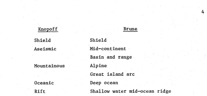
operational), are summarized by Knopoff [1972], who groups the data into five geophysical regions, and also by Brune [1969], who uses seven

Knopoff Brune Shield

Aseismic

Mountainous

Oceanic Rift

Shield

Mid-continent Basin and range Alpine

Great island arc Deep ocean

Shallow water mid-ocean ridge

Knopoff cites over 50 studies of direct observations that yield phase velocities to periods longer than 60 s; he does not summarize the more numerous studies of dispersion at shorter periods. Fig. 1.1, reproduced from Knopoff, shows the Rayleigh wave spans for his five groupings. Inversion of typical phase velocity curves from each of the five groups established markedly different shear velocity profiles in the upper mantle. The low velocity channel is absent, or nearly so, under shield areas. In the other regions,its depth and velocity contrast with layers above and below it are not known in detail. Completely unknown is the distance over which the change in structure takes place.

1.2 ANALYTICAL METHODS FOR OBTAINING PHASE AND GROUP VELOCITY

There have been a number of recent significant advances in digital methods of obtaining surface wave dispersion information from seismograms. The treatise by Dziewonski and Hales [1972] gives a

comprehensive discussion of all the methods of numerical analysis used to obtain phase and group velocities from observed seismic signals.

In a series of papers Satö [1955, 1956, 1956] introduced Fourier analysis to surface wave studies and demonstrated that phase velocity could be measured in non-dispersive propagation, where the peak and trough method fails completely. Using a tripartite net to determine the direction of propagation of surface waves, Evernden [1953, 1954] showed that interference by waves refracted at oceanic-continental

boundaries was responsible for the pulse-like departures from the smooth wave-trains predicted by theory. Variations in the Moho depth in

Southern California were obtained by Press [1956], who developed the tripartite array technique, in which three stations are used to obtain phase velocity. This eliminated the necessity for the epicenter to be on some particular great circle path, and consequently more earthquakes could be used for analysis. The method, however, ignores azimuthal variations in the source function, which may introduce error.

Time-variant filters were introduced by Pilant and Knopoff [1964] to separate interfering dispersed wave trains. The interference can result from spatial or temporal separation at the source or from multipath propagation from a single source. The study of the Alpine region by Knopoff, Mueller and Pilant [1966] emphasized the difficulty involved in obtaining smooth phase velocity curves even when a high quality seismic net was used to gather data. Multipath propagation has been studied by Capon [1970, 1971], and Capon and Evernden [1971], using high resolution wave number analysis techniques on data supplied by LASA (the Large Aperture Seismic Array in Montana) to determine the direction of approach of propagating long period waves.

The combined use of time-variant filtering and Fourier analysis has been applied to many of the latest surface wave studies; the results of these studies are summarized by Knopoff [1972], who also gives an extensive source list.

analysis' by Landisman, Dziewonski and Satd [1969], who developed computer programs that convert a time series into a two-dimensional display of filtered signal amplitude (using either a linear or decibel scale) with group velocity or group arrival time plotted against the logarithm of period. The amplitude values are contoured by hand, and modes of propagation and group velocity can be inferred from the resulting contour diagram. This paper also introduced the concept of using cross-correlation of seismograms observed at two stations colinear

(in the great circle sense) with the earthquake epicenter to determine phase velocity and group velocity.

The next advance in computer-based analysis was 'multiple filter analysis' [Dziewonski, Bloch and Landisman, 1969] which exploited the Fast Fourier Transform [Cooley and Tukey, 1965] and eliminated a phase shift problem intrinsic in moving window analysis, whilst retaining the same form for presentation of results. Filtering is performed in the frequency domain instead of the time domain. These methods are

mathematically equivalent, and give essentially identical results. Recently, several papers have extended 'multiple filter analysis'. Levshin's [1972] critique of the process gives an

illustration of its noise-penetrating power, and also gives algorithms for speeding up the computations. Inston, Marshall and Blarney [1971] and Cara [1973] use the dispersion of the medium to obtain filter bandwidth variation with frequency for the purpose of maximizing the temporal resolution, although the 'residual dispersion' method [Dziewonski, Mills and Bloch, 1972] accomplishes the same end.

Bloch and Hales [1968] introduced some new techniques for the direct determination of phase velocity from seismograms recorded at a pair of stations, using a two-dimensional display similar to the multiple filter analysis of Dziewonski

et al.

concise acronym will be used throughout this dissertation. FTAN has been used extensively in this study to obtain group velocity from cross-

1.3 INVERSION

The ultimate goal of surface wave studies is to interpret the observed dispersion information in terms of possible structures and compositional properties of the Earth which have the same wave

propagation characteristics as the observed data. It is recognized that there is a high degree of non-uniqueness associated with the inversion problem; i.e., there exist a multiplicity of different structures possessing dispersion characteristics which satisfy the data. An

objective of inversion is to establish the possible existence of globally distinct (G-far) solutions, as opposed to solutions that differ only in their fine structure. An Earth model containing two low velocity

channels would be globally distinct from a model with only one low velocity channel.

The longer the period of Love or Rayleigh waves, the more deeply they penetrate into the Earth. Anderson’s [1964] Universal Love wave dispersion tables, computed via a variational approach combined with Haskell's [1953] matrix formulation, show that layers down to a depth of 1/2 to 1/6 of the surface wavelength have the most powerful influence on the phase velocity of the fundamental mode of Love waves. Similar

studies give a corresponding factor of about 0.4 times surface wavelength of Rayleigh waves [Knopoff, 1972].

Early inversion attempts used a trial and error method of adjusting a starting Earth model to fit the observed data within some level of tolerance. A systematic procedural basis for the trial and error method is described by Haddon and Bullen [1969]. Worthington

[1973] invokes 'the Principle of Maximum Simplicity' (which could also be termed 'the Principle of Least Astonishment') to describe the guiding rationale that leads to the least complicated model. The result of the trial and error method is a single model whose usefulness depends on the perseverance, intuition and judgement of the investigator.

With a single 'best' model as the defined objective of inversion, Dorman and Ewing [1962] used a least-squares curve-fitting technique and computed shear velocity partial derivatives at each step of the iterative procedure. Brune and Dorman [1963] employed the same

period and higher mode Rayleigh wave data, as well as fundamental mode Love wave data. However, subsequent studies showed that their least-squares curve-fitting could create numerical instabilities [Takeuchi and Sudo, 1968; and Takeuchi, Dorman, and Saito, 1964].

Backus and Gilbert [1967, 1968, 1970] have formally examined the non-uniqueness of the general inverse problem of determining the structure of the Earth from free oscillation data. Since their mathematics is formidable, Parker [1970] may be read for a clear

exposition of their work in relation to electrical conductivity in the mantle.

The Monte Carlo method, as first presented by Keilis-Borok and Yanovskaya [1967], puts the trial and error method of inversion on a firm statistical basis. Although demanding large amounts of computing time, Monte Carlo inversion gives a family of models that satisfy the observed data to some given level of accuracy; see for example, studies by Press

[1968], Wiggins [1969], Anderssen, Worthington and Cleary [1972].

The envelope of all acceptable models produced by a Monte Carlo run can be achieved with significantly less computing expenditure by linear-programming techniques, as first applied to the geophysical

problem by Johnson [1972] and later used by Worthington [1973]. However, LP inversion has been criticised for two reasons: (1) its complete

reliance on the assumption of validity of linearization of the problem and (2) the extremal character of the derived models.

The poristic nature of the inverse problem in geophysics makes it difficult to see direct relations between the observed data (e.g., standard deviations, phase or group velocity, amplitude information) and the non-uniqueness bounds of possible solutions. Wiggins [1972] has studied this problem and uses the eigenvectors of the coefficient matrix to establish the resolving power and information distribution of free oscillation data. A pragmatic approach used by Dziewonski [1971] attempts to match 'pure path' dispersion information for Love and

Rayleigh waves in the period range 150 to 325 s with models characterized by the smallest possible number of parameters. He showed that the

distribution of shear velocity and density in the first 400 km may be adequately described by a set of four values corresponding to: (1) crust,

to the 400 km discontinuity. In an earlier paper Dziewonski [1970a] showed that a high (negative) correlation exists between shear velocity partial derivatives and density partial derivatives in the upper mantle; non-uniqueness stems partly from this correlation since the computed functionals can be fitted to observed data by changing either density or shear velocity in the appropriate manner.

It may be noted here that difficulties have occurred in attempts to fit both Love and Rayleigh wave data simultaneously to a model. This problem was first encountered by McEvilly [1964] who

proposed: (1) erroneous Love wave data, or (2) anisotropy (differences between horizontal and vertical shear velocity) as possible explanations for the problem.

Der

et al.

observations yield much less information than Rayleigh waves about the shear velocity distribution, and that higher mode observations increase the accuracy and resolution that may be attained. Furthermore,

'the most difficult part of conducting such a study is the estimation of errors. The propagation of errors in complicated digital processing and filtering operations, inability to

estimate the effects of lateral refraction and lateral changes in the structure, and errors caused by instrumental phase shift all contribute to the overall measurement error in varying and often unknown amounts'.

1.4 THE PRESENT STUDY

In 1963 there were five WWSSN stations operating in Australia: TAU-Hobart, MUN-Mundaring, CTA-Charters Towers, RIV-Riverview and

ADE-Adelaide, making nine station pairs available for surface wave

studies in this continent. (Permutation of five stations taken two at a time actually gives ten paths, but one of them, Hobart to Mundaring, is oceanic and will not be considered further.)

There have been few surface wave studies of the Australian continent. The author is aware of only two works that have looked for regional differences in Australia by this method, those of Bolt and Niazi

seismograms recorded at Perth, Brisbane and Charters Towers from earth­ quakes in the seismic belt from Banda Sea to Noumea. They used the peak and trough method to cover the period range 14 to 25 s for group

velocities and 14 to 45 s for phase velocities of Rayleigh waves. They concluded that the crust of the path from Charters Towers to Perth closely resembles the structure of the Canadian Shield as determined by Brune and Dorman [1963]. But they noted the presence of regional

differences in the Australian crust and a systematic decrease in group velocity between 15 and 25 s as the path from the selected earthquakes to Perth became more northerly. On the basis of Rayleigh wave dispersion, they concluded that the overall crustal thickness of Australia was probably between 30 and 35 km. The relatively short span of periods of their dispersion information does not permit investigation of the

structure of the upper mantle.

Thomas selected a set of 35 earthquakes and attempted to

ascertain if two-station analyses of Rayleigh waves over these nine paths would reveal any regional differences in surface wave dispersion. He

used a variation of the peak and trough method to obtain phase velocities and this limited the maximum period to 50 s, at best. Although a

large number of events were successfully analysed, the scatter of the data prevented any definite conclusion about regional differences. Using Dorman and Ewingfs [1962] inversion methods on polynomial smoothed data, Thomas concluded that: (1) if the crust were considered to be a uniform single layer the data indicated a Moho depth that was constant within 5% over the whole continent; and (2) if two layers were used in the

starting model, the data would indicate considerable variation within the crust, although the depth of the Moho would be within 1 km of 40 km over the continent. It was obvious that inversion of fundamental

Rayleigh wave phase velocities alone did not allow the crust-mantle structure to be uniquely determined.

Thus, in 1969, little was known about surface wave propagation across Australia. Love wave studies had never been attempted, and

Rayleigh wave information was sparse and scattered, no information other than that for the path CTA-ADE was available for periods longer than 50 s

objectives of: (1) extending the period range of Rayleigh wave

information by using the recently developed numerical methods discussed in Section 1.2; (2) obtaining Love wave dispersion data; and

(3) inverting this new information to establish possible crust-mantle structures. A concomitant more general objective was to attempt to extend the analysis range of direct surface wave observations to longer periods so that they would overlap with the average regional data

obtained from studies of circumferential traverses and free oscillations.

The original set of earthquakes used by Thomas was re-examined. Early results obtained by summing cross-correlations looked promising, but indicated that more events with differing epicentral distances would have to be included in the summation of cross-correlograms in order to realize the full noise-reducing capability of this technique. The study was therefore expanded and seismograms from an additional 100 events were obtained from the Seismological Data Center, Washington, D.C. Particular attention was paid to the inclusion of earthquakes on both sides of a two-station pair. Group velocity was obtained over the period range 10 to 183 s, and phase velocities were derived both by integrating the group velocity and by Fourier analysis. Very smooth phase velocity curves are obtained by integrating group velocity. To the author’s knowledge the method of obtaining phase velocity by integrating group velocity (see Chapter 3) has not been used in published surface wave studies. An explanation for its absence probably stems from the fact that group velocity is generally more susceptible to noise than is phase velocity. The discussion in Chapter 4 shows that further signal averaging can be obtained by combining the Frequency-Time-Analysis results for different paths belonging to the same regions, but this averaging does not permit the direct extraction of phase velocity by Fourier analysis. It does however yield an unbiased average of group velocity, which can then be integrated to obtain phase velocity.

The following chapter describes the methods used for data

surface wave dispersion across Australia and clearly shows differences between dispersion across western and eastern Australia. The problem of interference between the fundamental Love mode and higher Love modes is examined, and it appears that the method of summing cross-correlations gives a reasonably accurate measurement of Love wave phase velocities. Chapter 5 describes the Monte Carlo inversion of the dispersion results and presents feasible Earth models for western and eastern Australia.

CHAPTER 2

DATA ACQUISITION AND DIGITIZATION

Dziewonski and Landisman [1970] applied cross-correlation

concepts, originally proposed by Landisman

et al,

(the two-station method) first appears in Dziewonski and Hales [1972]. The advantage of this method is that it affords a means of enhancing the phase information contained in seismograms before performing the non­ linear operation of computing $(a)) = arctangent [ ImF(o))/Rc.F(w) ], where F(co) is the complex Fourier spectrum of either: (1) a station seismogram, or (2) a cross-correlogram of two seismograms. Apparently this method of summing cross-correlograms has not yet been used in published two-station studies of surface waves. To the author's knowledge, all surface wave studies appearing in the literature compute the phase curve for each event separately before averaging the results.

A deteriorating signal/noise ratio at longer periods causes the computational efficiency of $(u)) to deteriorate. By summing cross-

correlograms, the signal/noise ratio is enhanced, particularly at longer periods. Destructive interference of signal-organized noise is achieved by including events with differing epicentral distances in the sum of

cross-correlograms.

2.1 DATA SELECTION AND ACQUISITION

Phase and group velocity are obtained from surface waves

epicenter

great c i r c l e pathgrea

i

station

1

st at i on

2

Figure 2.1: Sketch of two-station method.

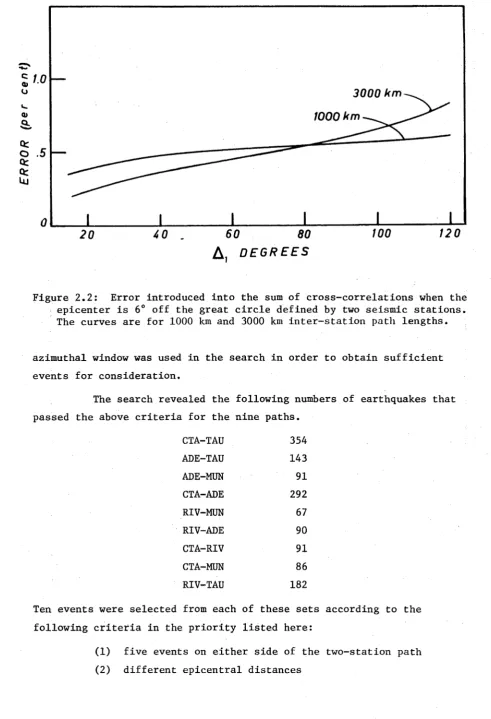
at station 1, and with magnitudes greater than 5.5 (see Fig. 2.1). Knopoff and Schwab [1968] show that source phase shift is frequency-dependent and is also a function of the inclination of the source from the vertical. Thus, it is important to minimize the displacement of the epicenter from the great circle colinear with the two observing stations. The method of summing cross-correlations assumes that the event lies exactly on the great circle path defined by the locations of the two seismic observatories. If this assumption is not strictly true, an error related to the difference between the differential path length and the distance between the two stations is introduced. The error increases as the epicenter is located further off the great circle, and a similar error can be introduced in the case of very deep earthquakes. Fig. 2.2 shows the magnitude of the error. Events with locations that would have caused a gross error by being too far off the great circle were not

included in the sum of cross-correlograms. This criterion prevented some of the events in Thomas's list from being included in the sum of cross­ correlations. For example, his event number 31 lies 16° off the great circle connecting CTA-MUN. Correct phase velocities for these events can be obtained by using the proper differential path length in the

computation of velocity [see Thomas, 1969], although source phase shift might introduce an error if the deviation is excessive.

3000 km

WOO km

40

A,

D E G R E E S

Figure 2.2: Error introduced into the sum of cross-correlations when the epicenter is 6° off the great circle defined by two seismic stations. The curves are for 1000 km and 3000 km inter-station path lengths.

azimuthal window was used in the search in order to obtain sufficient events for consideration.

The search revealed the following numbers of earthquakes that passed the above criteria for the nine paths.

CTA-TAU 354

ADE-TAU 143

ADE-MUN 91

CTA-ADE 292

RIV-MUN 67

RIV-ADE 90

CTA-RIV 91

CTA-MUN 86

RIV-TAU 182

Ten events were selected from each of these sets according to the following criteria in the priority listed here:

(3) large magnitude

(4) small great-circle azimuthal deviation.

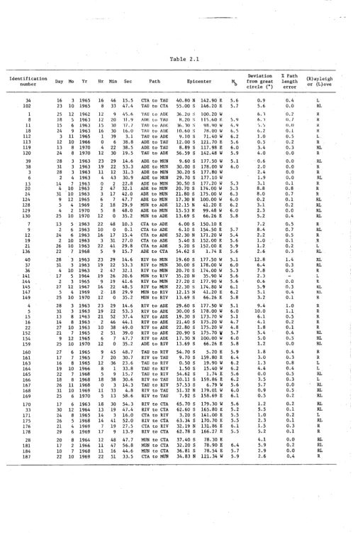
Copies of the vertical and horizontal component seismograms on 70 mm film chips were ordered from the Seismological Data Center, Washington, D.C. The full list of the earthquakes used in this study appears in Table 2.1. Event identification numbers from 1 to 40 correspond to the same

numbering scheme used by Thomas. The numbers above 100 represent additional events. Fig. 2.3 shows the locations of these events on a stereographic projection of the Earth centered at Alice Springs (which is nearly the geographical center of Australia). The nature of the highly

15,1 6,

22,152 2 0,24,36,145

•124,129

130,149,159

3.6.13.38,39.4.5,4 0.37

S O U T H

POLEt

1,11,18,112 ■160, 165,167

163,164

Table 2.1

Identification

number Day Mo Yr Hr Min Sec Path Epicenter “ b

Deviation % Path from great length circle (°) error

(R)ayleigh or (L)ove

34 16 3 1965 16 46 15.5 CTA to TAU 40.80 N 142.90 E 5.6 0.9 0.4 L

102 23 10 1965 8 33 47.4 TAU to CTA 55.00 S 146.20 E 5.7 5.6 0.0 RL

1 25 12 1962 12 9 45.6 T A D t o ADE 36.20 s 100.20 W 6.3 0.2 R

8 18 5 1963 12 20 31.9 A DE l oT A D 8.20 s 115.60 K 5.9 6. 1 (I. ! K

11 15 6 1963 15 30 37. / T A D to ADE 16. 30 s 98.90 W 4.9 5.5 0.0 l<

18 24 9 1963 16 30 16.0 T A D to ADE 10.60 s 78.00 w 6. 6 6.2 0.1 K

112 3 11 1965 1 39 3.1 TAU to ADE 9.10 s 71.40 w 6.2 I .0 0.5 L

113 12 10 1966 0 6 38.8 ADE to TAU 12.00 s 121.70 E 5.6 0.5 0.2 R

119 13 8 1970 4 22 38.5 ADE to TAU 8.89 s 117.98 E 6.0 3.4 0.3 RL

120 24 8 1970 12 30 19.5 TAU to ADE 56.59 s 142.48 W 5.9 4.0 0.0 R

39 28 3 1963 23 29 14.6 ADE to MUN 9.60 s 177.50 W 5.1 0.6 0.0 RL

38 31 3 1963 19 22 53.3 ADE to MUN 30.00 s 178.00 W 6.0 2.0 0.0 R

3 28 3 1963 11 12 31.3 ADE to MUN 30.20 s 177.80 W 2.4 0.0 R

6 2 4 1963 4 43 30.9 ADE to MUN 29.70 s 177.10 W 1.9 0.0 RL

13 14 7 1963 0 2 22.8 ADE to MUN 30.50 s 177.20 w 5.3 3.1 0.1 R

20 4 10 1963 2 47 32.1 ADE to MUN 20.70 s 174.00 w 5.3 8.8 0.8 R

24 31 10 1963 3 17 42.0 ADE to MUN 21.80 s 175.00 w 6.3 8.0 0.7 R

124 9 12 1965 6 7 47.7 ADE to MUN 17.30 N 100.00 w 6.0 0.2 0.1 RL

128 5 4 1969 2 18 29.9 MUN to ADE 12.15 N 41.20 E 6.2 3.1 0.2 RL

129 4 2 1970 5 8 48.0 ADE to MUN 15.53 N 99.48 W 6.0 2.3 0.0 RL

130 25 10 1970 12 0 35.2 MUN to ADE 13.69 s 66.26 E 5.8 5.2 0.4 RL

7 13 5 1963 22 48 10.3 CTA to ADE 6.00 s 150.10 E 7.2 0.5 R

9 2 6 1963 10 0 0.1 CTA to ADE 6.10 s 154.50 E 5.7 8.4 0.7 RL

12 24 6 1963 16 17 15.4 CTA to ADE 52.30 N 171.20 W 5.4 2.2 0.5 R

19 2 10 1963 3 31 27.0 CTA to ADE 5.40 s 152.00 E 5.6 1.0 0.1 R

21 26 10 1963 22 41 29.8 CTA to ADE 5.20 s 152.00 E 5.9 1.2 0.2 L

136 22 7 1968 5 9 15.7 ADE to CTA 54.62 s 1.74 E 5.6 2.6 0.3 RL

40 28 3 1963 23 29 14.6 RIV to MUN 19.60 s 177.50 W 5.1 12.8 1.4 RL

37 31 3 1963 19 22 53.3 RIV to MUN 30.00 s 178.00 W 6.0 6.4 0.3 RL

36 4 10 1963 2 47 32.1 RIV to MUN 20.70 s 174.00 W 5.3 7.8 0.5 R

141 17 5 1964 19 26 20.6 MUN to RIV 35.20 N 35.90 W 5.6 2.3 - L

144 2 3 1965 9 19 41.6 RIV to MUN 27.20 s 177.90 W 5.6 0.6 0.0 R

145 27 12 1967 16 22 48. 5 RIV to MUN 22.30 s 174.80 w 6.1 5.9 0.3 RL

147 5 4 1969 2 18 29.9 MUN to RIV 12.15 N 41.20 E 6.2 5.1 0.4 HI.

149 25 10 1970 12 0 35.2 MUN to RIV 13.69 s 66.26 E 5.8 3.2 0.1 R

4 28 3 1963 23 29 14.6 RIV to ADE 29.60 s 177.50 W 5.1 9.4 1.0 R

5 31 3 1963 19 22 53.3 RIV to ADE 30.00 s 178.00 W 6.0 10.0 1.1 R

15 13 8 1463 21 52 37.4 RIV to ADE 19.30 s 173.70 w 5.1 6.1 0.5 R

16 14 8 1963 2 46 44.1 RIV to ADE 21.40 s 175.20 w 4.7 4.1 0.2 R

2 2 27 10 1963 10 38 49.0 RIV to ADE 22.80 s 175.20 w 4.8 1.8 0.1 R

152 21 7 1965 2 51 39.0 RIV to ADE 20.90 s 175.70 w 5.7 5.4 0.4 RL

154 9 12 1965 6 7 47.7 RIV to ADE 17.30 N 100.00 w 6.0 5.0 0.5 RL

159 25 10 1970 12 0 35.2 ADE to RIV 13.69 s 66.26 E 5.8 1.2 0.0 RL

160 27 6 1965 9 45 48.7 TAU to RIV 54.70 s 5.20 E 5.9 1.8 0.4 R

161 17 7 1965 7 20 30.7 RIV to TAU 9.70 s 159.80 E 6.4 3.0 0.3 R

163 16 8 1965 12 36 23.6 TAU to RIV 0.50 s 19.90 W 6.2 1.3 0.8 L

164 19 10 1966 8 1 33.8 TAU to RIV 1.50 s 15.40 W 6.2 4.4 0.4 L

165 22 7 1968 5 9 15.7 TAU to RIV 54.62 s 1.74 E 5.6 0.0 0.5 RL

166 18 8 1968 18 38 30.6 RIV to TAU 10.11 s 159.86 E 6.2 3.5 0.3 L

167 26 11 1968 0 3 14.3 TAU to RIV 57.53 s 6.79 W 5.6 5.7 0.0 RL

168 31 10 1969 11 33 4.8 RIV to TAU 51.32 N 179.01 W 6.0 0.9 0.5 RL

169 25 6 1970 5 13 58.6 RIV to TAU 7.92 s 158.69 E 6.1 0.5 0.2 RL

170 17 6 1963 18 30 54.3 RIV to CTA 65.70 s 179.30 U 5.6 1.2 0.2 RL

33 30 12 1964 13 19 47.4 RIV to CTA 62.60 s 165.80 E 5.2 5.5 0.1 RL

171 24 8 1965 14 3 16.0 CTA to RIV 3.20 s 141.00 E 5.5 1.0 0.2 L

175 26 5 1968 14 41 52.0 RIV to CTA 63.34 s 170.70 E 5.5 2.3 0.1 RL

176 21 4 1969 7 19 27.5 CTA to RIV 32.19 N 131.86 E 6.1 1.5 0.3 R

178 29 6 1969 17 9 13.9 RIV to CTA 62. 78 s 166.27 E 5.5 5.2 0.1 R

28 20 8 1964 12 48 47.7 MUN to CTA 37.40 s 78.30 E 4.1 0.0 RL

181 17 2 1966 11 47 56.8 MUN to CTA 32.20 s 78.90 E 6.4 5.9 0.2 RL

184 10 7 1968 11 16 44.6 MUN to CTA 36.81 s 78.54 E 5.7 2.9 0.0 RL

structured seismic activity of the Earth is apparent. Most earthquakes occur in small belts of activity, and thus a restriction is imposed on fulfilment of the condition that surface waves from a full range of epicentral distances be cross-correlated and summed for each two-station path.

It is worthwhile to point out the necessity for continual scrutiny in the data-preparation stage. For example, Thomas’s events 34 and 35 produced virtually identical seismograms at both CTA and TAU even though the second event occurred 13 days after the first. There would be no signal/signal-generated-noise enhancement derived from analysing both events. The possibility of analysing replicate seismograms is reduced if, within an active seismic zone, events are chosen for maximal separation and this precaution was observed throughout the data-selection stage.

The above selection criteria provided 90 events suitable for further processing. Since a two-station analysis of both Love and Rayleigh waves requires digitization of six seismograms for each event, there were potentially 540 more seismograms to be digitized. Clearly, some thought had to be given to methods of digitization and management of this large amount of data, or the capabilities of a single investigator would have been inadequate. The next section in this chapter describes how an efficient digitizing method was developed for this project.

It is perhaps first necessary to discuss the reasons for

analysing so much data when, in principle, 'a single seismogram contains all the information needed for a fairly detailed structural

interpretation' [Anderson, 1967, p.360]. The primary reason is, of course, the objective of extending the range of reliable phase velocity measurement, hopefully to a period as long as 200 s. Great earthquakes, particularly deep ones, are efficient generators of mantle (i.e. mantle­ sensing) waves; the problem is that the trace of the direct observation of the waves from great earthquakes is almost always driven off-scale by the magnitude of ground motion, so that the earlier signals of world-circling waves usually cannot be read. Therefore we are forced to use seismograms from smaller earthquakes, in which mantle-wave amplitudes may be so small as to be imperceptible by visual examination. Only by

At shorter periods, although the signal strength is high, the seismogram may be contaminated by signal-organized noise. Thomas's phase measurements became rather scattered and unreliable above 40 s for some paths. In gathering dispersion information, the common practice has been to examine a number of records to obtain for analysis those that contain clear dispersed wave trains with minimal evidence of beats indicating refraction. But what if no such clear records are ever observed?

An example is the CTA-TAU path. No clear vertical component records from events located north of CTA were observed, but the events located south of TAU generated relatively clear signals at both TAU and CTA. There are probably other station locations on the Earth where, for similar reasons, clear uncontaminated wave trains are not observed, and in these cases signal enhancement processing methods by summing many records would be of great use.

Some of the sources of noise contamination of long period records are:

(1) refraction at continental boundaries causing later arrival of energy at either or both stations.

(2) multi-path propagation or reflection from continental boundaries [see Capon, 1970, 1971].

(3) multiple or extended source functions in time and space that generate overlapping wave trains.

(4) higher mode propagation.

(5) contamination by body waves; for example, core

reflections can arrive in the midst of a dispersed surface wave train.

(6) seismic and instrumental background noise, significant in the low-amplitude portions of the signal spectrum.

analysis of this cross-correlogram in Fig. 3.4 shows anomalously high group velocity at 21 s. Furthermore, the ridge crest that defines group velocity is disturbed between 20 and 30 s. The processing used to

generate these FTAN diagrams is described in Chapter 3.

2.2 DIGITIZING AND MANAGEMENT OF DATA

In view of the lack of digitizing facilities in Canberra

suitable for processing the large number of records required in the study, a digitizing program was developed about a PDP-15 computer and its

peripheral devices, primarily a 12-bit A/D converter and a Calcomp Model 565 Incremental Plotter. Initially, this computer had 16 K words of memory (later upgraded to 32 K ) ; its use was restricted to staff and students of the Department of Engineering Physics. Any limitations imposed by its relatively small size were found to be compensated by its availability and by the close supervision of the processing stream

afforded by the single-user concept. This computing installation provided on-line graphical interaction with the data processing, with both hard and soft copy available as output. The need for quick graphical output in seismic data processing work can hardly be over­ stressed. This kind of ’hands on' service is seldom available at large multi-user computing centers.

Digital Equipment computers use file-oriented Dectape for semi­ permanent storage of programs and data. A standard format was used that denoted the number of the event, the name of the recording station and the seismograph component in the title of the file. The file contained a 1024-point digitized seismogram, the start time of digitizing and

information about the sampling rate. This data-management system avoided the bulk associated with cards and paper tape, and there was less chance of mistaken identification of data files than in storage on magnetic tape.

The following sections (extracted from the author’s paper 'Computer-Aided Digitization of Chart Records’, published in Journal of

Physics E , Jan, 1974) describe the PDP-15 digitizing system and also

2.3 DIGITIZING INSTRUMENTS

Commercial XY-digitizing instruments increment along one axis, and when a predetermined sampling point is reached, record signal

displacement perpendicular to that axis. They are suited to the

digitization of chart records with rectilinear, orthogonal axes. However many recording instruments do not operate in this orthogonal, rectilinear mode: for example, more data can be recorded on the same area of paper by writing the trace on a recording medium that has been wrapped around a rotating drum, which is being continuously advanced by a lead screw.

This helical recording mode is used by many observatories to record continuously the variation of some quantity (such as ground motion) and in particular is used by the World-Wide Standard Seismic Network to obtain a complete day's earthquake activity on a single manageable record

Two points arise when these signals are to be digitized: (1) the time axis is not parallel to the edge of the paper; (2) the signal axis is not perpendicular to the time axis. The angle between the signal axis and the time axis differs from 90° by the pitch of the lead screw that advances the drum; let this angle be 0 . Although 0o is usually rather small, typically only 0.3° in WWSSN recordings, James and

A

Linde [1971] showed that significant errors can be introduced into any subsequent Fourier analysis if it is ignored during digitizing.

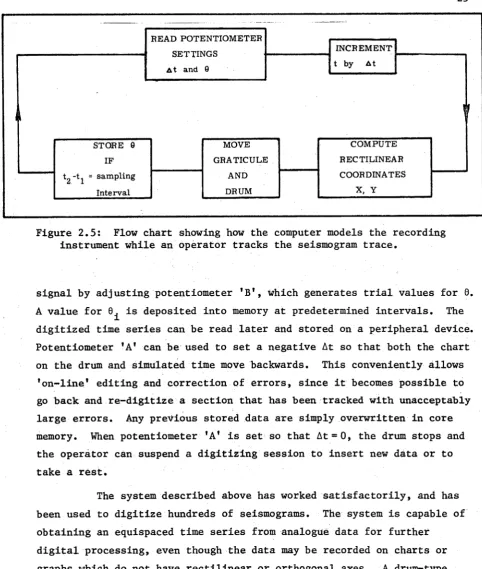
A serious digitizing problem occurs when chart records are made on instruments in which the pen is directly attached to a moving-coil galvanometer. The signal axis is curvilinear instead of rectilinear, because the pen is constrained to move in a circle with radius equal to the length of the galvanometer arm. When this type of chart record is digitized with a rectilinear-digitizing instrument, the signal can sometimes erroneously appear to be multiple-valued. The proper digitization of this type of chart record is a time series of the galvanometer deflection angle 0^ at discrete time intervals t^.

Table 2.2 lists the characteristics of four common types of recording instruments and Fig. 2.4 shows how their axes are arranged.

Type Galvanometer arm length

Usual offset angle (°)

Type of trace (see Fig. 2.4)

XY recorder effectively

infinite 0 Straight (a)

Drum 1 m 0.3 Straight (c)

Drum (heated stylus) 7 in 1.7 Curved (d)

Portable strip chart 2 in 0 Curved (b)

Figure 2.4: The appearance of the axes of some types of recording

instruments. (a) XY recorder, (b) strip chart recorder, (c) drum in helical recording mode with light beam, (d) drum and heated stylus, s is signal axis, t is time axis.

signal with a microscope. They found that variable drum speed and

sampling interval, and optical magnification, were features that improved accuracy as well as reduced the associated tedium. Goodspeed and Savage

[1968] describe an electromechanical digitizer designed to process large amounts of meteorological data.

Experience has shown that certain human engineering factors should be considered when designing a digitizing system. It is