Theses
Thesis/Dissertation Collections
5-1-1999
Paramaterized beams as effective human lip models
Ron Dufort
Follow this and additional works at:
http://scholarworks.rit.edu/theses
This Thesis is brought to you for free and open access by the Thesis/Dissertation Collections at RIT Scholar Works. It has been accepted for inclusion
in Theses by an authorized administrator of RIT Scholar Works. For more information, please contact
Recommended Citation
EFFECTIVE HUMAN LIP MODELS
by
Ron Edward Dufort
A Thesis Submitted
III
Partial Fulfillment
of the
Requirement for the
MASTER OF SCIENCE
IN
MECHANICAL ENGINEERING
Approved by:
Professor Mark H. Kempski
Department of Mechanical Engineering
Professor Richard G. Budynas
Department of Mechanical Engineering
Dr. Risa 1. Robinson
Department of Mechanical Engineering
Professor Charles W. Haines
Deparment of Mechanical Engineering
(Thesis Advisor)
(Committee Member)
(Committee Member)
(Department Head)
DEPARTMENT OF MECHANICAL ENGINEERING
ROCHESTER INSTITUTE OF TECHNOLOGY
Abstract
There
are numerous mathematical equations used
by
animators and modelers
to
describe
the
curves of
the
human face
and, specifically, the
human
Up.
Physically-based
polynomial
models,
b-splines,
and other
arbitrarily
parameterized equations are used
to
describe facial
and
Up
contours,
though
with varied
degrees
of
complexity
and resolution.
This study
examined
the
constraints and conditions
necessary
to
utilize a standard
Euler-BernoulU beam
as
an effective model
for
the
human Up. Through
this
analysis
it
was
determined
that
general
beam
theories
are
flexible
enough
to
create models
that
can generate curves comparable
to
actual
lip
shapes,
though
no single model studied was
appreciably
better
suited
for
aU
possible
Up
shapes.
Such
models could
stiU,
however,
be
utilized
in
the
development
of
computer-based animation as
weU
as motion
tracking
systems,
computer user
interfaces,
and
teleoperational
devices. Beam
characteristics such as cross sectional
shape,
length,
and
elasticity
were
investigated in
order
to
define deflection
models
for four
different
beam
configurations: a
clamped prismatic
beam,
a
simply
supported prismatic
beam,
a clamped
tapered
beam,
and a
simply
supported
tapered
beam.
Multiple beam
loading
scenarios
were
simulated
to
determine
the
optimal number and arrangement of
loads
to
reproduce
the
desired deflection
curves.
Deflection
curves
defined
by
each of
the
four beam
models
were
compared
to
actual
deflection
curves
digitized from
photographs of
the
human
Up
and
have
been
presented
here.
Permission
I, Ron Edward Dufort, hereby grant permission to the Wallace Memorial Library of the
Rochester Institute of Technology to reproduce my thesis entitled Parameterized Beams as
Effective Human Lip Models
in
whole or
in
part. Any reproduction will not be for
commercial use or profit.
Ron Edward Dufort
Acknowledgements
Through
the
many hours
spent
devising, developing,
and
polishing
this
thesis,
my
family
at
home
stood always
by,
patient,
encouraging,
and at
exactly
the
right
times
demanding.
My
friends in
Rochester, NY,
who
are also
my
family,
did
the
same.
To
aU of
them
I
owe a great
debt
of gratitude.
I
would not
have had
the
determination
to
finish
this
alone.
To
the
many
teachers
I have
come
to
know both professionally
and
privately,
who
have
taught
me about
engineering
and about
life,
I
also extend
my deepest
thanks.
You have
continued
to
inspire
me,
encourage
me,
and
demand
of me a
level
of
dedication I didn't know
I
could give.
Table
of
Contents
Abstract
Release
Acknowledgements
Table
of
Contents
Table
of
Symbols
List
of
Figures
List
of
Tables
List
of
Photographs
n
iii
iv
v
vu
ix
x
x
Literature Search/Background
1
1.1
Origins
of
Facial Animation
1
1.2
Lip
Models
4
1.3
The Beam
Theory
Connection
5
1.4
Goals
of
This Thesis
7
Formulation
of
the
Beam Model
8
2. 1
Identification
of
Possible Relevant
Conditions
8
2. 1
.1
Geometric/Material Properties
8
2.1.2
Constraining
Properties
8
2.2
Adaptation
of
Basic Beam
Bending
Equations
8
2.2.1
SimpUfication
of
Possible
Loading
9
2.2.2
SimpUfication
of
Possible
Constraints
10
2.2.3
SimpUfication
of
Possible Beam
Shapes
10
2.2.4
Other Assumptions
12
2.2.5
Summary
of
Beam
Cases
14
2.3
Calculation
of
Deflections
14
2.3.1
Case 1
15
6.
7.
2.3.3
Case 3
2.3.4
Case 4
2.4
Verifying
Type 2 Beam Models
Testing
Approach
3.1
Beam
Shape
3.2
Loading
Scenarios
3.3
Comparison
Criteria
Analyses
4. 1
Lip-Curve Data
CoUection
4.2
Model
Comparisons
4.2.1
One-Load Trials
4.2.2
Two-Lo
ad
Trials
4.2.3
Three-Load Trials
4.2.4
Four-Load Trials
4.3
Summary
Discussion
5. 1
Type 1
vs.
Type 2
-Prismatic Beams
vs.
5.2
Cases
1
and
3
vs.
Cases
2
and
4
-Clamped
5.3
Lip
Shapes
5.4
What Model When
Recommendations
Bibliography
17
20
22
23
23
23
23
25
25
27
29
32
35
38
41
42
43
43
44
44
45
47
Appendices
A
-Integrating Singularity
Functions
B
-Solving
a
System
of
Equations
C
-Determination
of
Iavg
D
-Lip
Measurements
E
-Microsoft
Excel'
s
Solver
Parameters
49
51
53
54
62
Symbols
Symbol
Name
Description
Units
Ci
Constant 1
c2
Constant 2
c3
Constant 3
E
Modulus
of
Elasticity
I
h
h
L
LP
M
Force
Moment
of
Inertia
Moment
of
Inertia
parameter
A
Moment
of
Inertia
parameter
B
Length
Length
in Photo
Moment
radius
x-axis
distance from
origin
to
location
of
load
x-axis
distance from
the
load
to
the
right edge of
the
beam
Constant
of
integration
Constant
of
integration
Reaction
moment at
point
A
on
the
beam
Ratio
of
Stress
to
Strain
within
Elastic limit
of
material
The
magnitude of
the
point
load
appUed at
a
Second
area moment
Scaling
parameter
for
I(x)
Shape
parameter
for
I(x)
Length
of
beam
model
Length
on photo of a
10mm
segment of
the
ruler
in
the
photo
Moment
Radius
of cylindrical
beam
mm
mm
10"3
rad
(im
N-mm
Gpa
N
mm4
6
mm
mm
mm
mm
N-m
mm
Ra
S
V
CCi
a?
Reaction Force A
Scale
Shear Force
y
alpha
1
alpha
2
Pi
beta 1
h
beta 2
Yi
gamma
1
Y2
gamma
2
Reaction
force
at point
A
on
the
beam
Scale
of photo
Shear force
at a given
point
along
the
beam
distance along
the
beam
(in
the
x-axis)
deflection
of
the
beam
(in
the
y-axis)
Coefficient
of
C3
in
Equation
(2.21)
Coefficient
of
C3
in
Equation
(2.22)
Coefficient
of
RA
in
Equation
(2.21)
Coefficient
of
Ra
in
Equation
(2.22)
Coefficient
of
P
in
Equation
(2.21)
Coefficient
of
P in
Equation
(2.22)
N
mm
N
mm
Hm*
mm
mm
mm
mm
mm
mm
*
y dimensions
appear as mm
in
simulations
-the
modulus of
elasticity
for
simulations was
taken
as
10"3GPa
so
deflections
would
be
on
the
mm
order of
magnitude.
List
of
Figures
Figure #
Figure Title
Page*
2.1
Three Transverse Point Loads
...2.2
Cylindrical Beam
with
Varied Radius
2.3
Beam
Case 1
2.4
2.5
Beam
Case 2
Beam
Case 3
2.6
Free
Body
Diagram
of
Beam
Case 3
2.7
Beam
Case 4
4.1(a)
Top
Lip,
Photo
#24,
Case 1
Model,
1 Load
4.1(b)
Top
Lip,
Photo
#24,
Case 2
Model,
1 Load
4.
1(c)
Top
Lip,
Photo
#24,
Case 3
Model,
1 Load
4.
1(d)
Top
Lip,
Photo
#24,
Case 4
Model,
1 Load
4.2(a)
Top
Lip,
Photo
#24,
Case 1
Model,
2 Loads
4.2(b)
Top
Lip,
Photo
#24,
Case 2
Model,
2 Loads
4.2(c)
Top
Lip,
Photo
#24,
Case
3
Model,
2 Loads
4.2(d)
Top
Lip,
Photo
#24,
Case 4
Model,
2 Loads
4.3(a)
Top
Lip,
Photo
#24,
Case
1
Model,
3 Loads
4.3(b)
Top
Lip,
Photo
#24,
Case 2
Model,
3 Loads
4.3(c)
Top
Lip,
Photo
#24,
Case 3
Model,
3
Loads
4.3(d)
Top
Lip,
Photo
#24,
Case
4
Model,
3 Loads
9
12
15
16
17
18
20
29
29
30
30
32
32
33
33
35
35
36
36
4.4(a)
Top
Lip,
Photo
#24,
Case 1
Model,
4 Loads
38
4.4(b)
Top
Lip,
Photo
#24,
Case 2
Model,
4 Loads
38
4.4(c)
Top
Lip,
Photo
#24,
Case 3
Model,
4 Loads
39
4.4(d)
Top
Lip,
Photo
#24,
Case 4
Model,
4 Loads
39
[image:11.566.63.470.59.634.2]List
of
Tables
Table #
Table Title
Page #
2.1
Beam
Configurations
14
4.1
One-Load
Summary
28
4.2
Two-Load
Summary
31
4.3
Three-Load
Summary
34
4.4
Four-Load
Summary
37
4.5
Summary
of
Optimized Sum
of
Squares
40
List
of
Photographs
Photo #
Photo Title
Page#
4.1
Scanned
Image,
Photo 24
25
4.2
Photo 24
with
Lip
Centerline
(dashed)
and
Actual
Lip
26
Curves
(dotted)
Shown
1.
Literature Search/Background
1.1
Facial
Animation
and
Modeling
Models
of
human physiology have
existed
for
centuries,
from
primitive
drawings
painted
onto cave walls
thousands
of years ago
to
DaVinci's
sketches of
the
human form drawn in
medical
reference
books in
the
1490's
to
three-dimensional
MRI
scans
displayed
on
digital
computers
in
the
1990's.
These
graphic
images
resemble aU or part of
the
human
body
and
aUow people
to
visuaUy
communicate
the
shape and
behavior
of
the
body.
The
creation and
control of
these
images
are
basic
goals of animation and modeling.
The Face
and
Communication
Since
the
face is important
to
basic
person-to-person
communication,
it has
always
been
of
special
interest
to those
who create graphic
models of
human beings [Magnenat Thalmann
1991]. A
stiU
image
of a
face
provides clues
to
personal characteristics such as
age, gender,
and current emotional state
[Whiteside 1974]. A moving
image
shows
those
characteristics
as
they
change over
time.
In
addition,
both
stiU
and
moving
images
can assist
in
language
comprehension
-the
interpretation
of vocal
language is
affected
greatly
by
visual
cues
including
mouth shape.
In
fact,
much
meaning
can
be inferred
solely from
mouth and
jaw
position,
without
any
sound at alL
It
is
the
chaUenge of
the
animator/modeler
to
develop
a
The
Face Image
The
specific appUcation of
the
model
determines
the
level
of
detail
required.
Cartoons
use
very
minimal
details
-features
are generalized
to the
point where
only basic
emotions such
as
happiness,
sadness,
and
frustration
can
be inferred. Visual
speech
recognition
is
not
possible
on
these models,
though
an animator
may
open and close
the
image
of
the
mouth
when
the
character
is
to
be
speaking;
this
cues
the
viewer
that
the
sounds are supposed
to
be
coming from
that
character.
For
some other
appUcations,
more
complex models are
desired
-models
that
possess
both
shape
characteristics and motion capabiUties of real
human
faces. These
require a clear
understanding
of
the
actual motions present
in
the
face
as weU as an accurate representation
of
the
geometry
of
the
face
and a control mechanism
that
manipulates
that
geometry in
ways
that
resemble
the
actual motions.
Because every
sighted person
is
accustomed
to
seeing
and
interpreting
faces
everyday,
even
the
smaUest
flaw in
the
animation or model can make
it
seem
wrong
to
a
viewer,
even
if
the
viewer cannot
identify
the
flaw. It is
therefore
important
to
have
the
most accurate models possible.
The Birth
and
Growth
of
Facial
Animation
In
1965,
Frederick
Parke
created
the
first
computer graphic models of
faces
[Parke
1996].
They
were
rudimentary
polygonal surfaces
that
resembled
faces opening
and
closing
their
eyes.
Through
the
late 1960's
and
early
1970's,
Parke
expanded
his
work
by
taking
polygon
data
of
actual
facial
expressions
to
create more
detailed
images
and
interpolating
between
those
images
to
create
the
illusion
of motion
-animation.
Other
researchers such as
Chernoff
and
GiUenson
worked on
two-dimensional
facial
models
during
this
time
[Parke
1996].
Another
researcher,
Henri
Gouraud,
developed
a smooth polygon
shading
technique
which
Parke
incorporated into
his
work and made
his
polygon
face
model more reaUstic.
By
1974,
Parke
had
taken
his
work
further
and
developed
a parameterized
facial
model
and
by
1980,
Piatt
at
the
University
of
Pennsylvania
succeeded
in creating
a
physically based
muscle-controUed
facial
expression model
[Parke 1996].
By
the
late 1980's
and
the
1990's,
parameterized
and muscle
based
models were
becoming
more
detaUed
and
more prevalent.
Aside from
the
basic
concerns
surrounding generating
images
on
computers,
much
of
the
research on computer
facial
animation
has focused
on
identifying
and
classifying
the
mechanisms
that
control
facial
motions.
Facial
motions are
generaUy
the
result of
expressions or speech.
The
activation of certain muscle groups
has been
related
to
specific
recognizable expressions
[Erkman
and
Rosenberg
1997]. Audio
cues
have
also
been
associated with
the
work of
specific muscle groups
-phonemes,
or
distinct
sound patterns
usually
related
to speech,
are coupled with specific mouth/Up/face shapes and orientations
known
as visemes.
Databases
such as
the
Facial Action
Coding
System
(FACS)
have been
created
that
relate
these
elements.
The FACS
has
been
an
invaluable
source of expression
information for
animators and
modelers since
its
creation
by
Paul Ekman
and
Wallace
Friesen in 1977 [Parke
1996,
Ekman
and
Rosenberg
1997].
Image
Creation
and
Control
According
to
Parke,
there
are at
least five
distinct
approaches
to
facial
animation:
interpolation [Parke 1996]. Performance
driven
and
interpolation
techniques
begin
with
digitized
images
of real
faces
and manipulate
them
according
to
either pre-designed
algorithms or control
inputs.
Pseudomucle- and muscle-based
techniques
use control
parameters
that
are related
to
simplifications of
the
actual
anatomy
of
the
face. Direct
parameterization
models
may be based
loosely
on actual muscle positions or
facial
configurations,
but rely mostly
on unrelated optimal parameters
for
controL
1.2
Lip
Models
The
Ups
are a smaU part of
the
overaU network of
muscles,
connective
tissue,
and skin
that
make
up
the
face. Most facial
models used
today
are at
least partiaUy based
on
the
physical
structure of
the
muscles and
bones
and
tissues
of
the
face [Parke 1996]. Since Ups
are
simply
the
fleshy
borders
to
a
flexible hole in
the
topology
of
the
face
they
could
be
overlooked
in
the
facial modeling
process;
they
could
be
accounted
for
as
the
edge
to the
skin model
that
surrounds
them.
This
is especially
true
when
considering
the
face
as a continuous surface as
is done
during
b-spline,
polygonal,
or other geometric-mesh models
[Magnenat Thalmann
1991].
In
these
types
of
models, the
curves and/or nodes
that
define
the
surface of
the
face
are moved
based
on
their
interactions
with
surrounding
elements
-various
muscles,
tendons,
and skeletal components.
This
provides
Up
motion and control without
directly defining
the
Ups
themselves.
A
more abstract
look
at
the
face
results
in very different
types
of models.
Each
component
such
as
the eye, the nose,
the
mouth,
or
the
ear can
be focused
on
individuaUy.
Often
a
basic
been
independently
modeled are added
[Parke 1996]. A
model can
then
be developed based
solely
on each component's
behavior,
not
necessarily
on
the
behavior
of
the
entire
face. The
upper
Up,
for
example,
can
be
modeled as
if it
existed alone
in
space.
The
completed
components
are
then
combined,
or
layered,
into
a single
face. A
cohesive model
is
achieved
by
coupling
the
motions of one component with
the
inputs
to
the
others,
so
lowering
the
jaw
would encourage
the
Ups
to
lower
as welL
Because
of
the
complexities
in
shape and motion of
the
Ups,
it is difficult
to
realisticaUy
model
them
no matter what approach
is
taken.
Lips
pose significant chaUenges
to
animators
kinematicaUy
as
weU
as
graphicaUy [Parke 1996]. Each distinct
mouth position
is defined in
part
by
a unique orientation and shape of
the
Ups;
during
speech
there
are
different
Up
shapes
related
to
certain
sounds.
However,
since sound
generation
is
only
partiaUy
affected
by Up
position,
different
sounds
may be
associated with
the
same
Up
configuration,
and
different
Up
configurations
may be
related
to
simUar sounds.
In
addition,
it is difficult
to
synchronize
Up
motions with speech and
facial
expressions
[Parke
1996].
It
is
therefore
desirable
to
derive
the
simplest model possible
that
allows quick
and
easy
calculation, control,
and
rendering
while
stiU
producing
reaUstic results.
1.3
The Beam
Theory
Connection
Considering
the
Ups
independently
from
the
rest of
the
face,
a
flexible
and
easily
manipulable set of shape equations
is
required
to
represent
the
many
possible shapes
the
Ups
facial
animations and models
is
beam-bending
equations.
Other
Up
models
have
utilized
the
flesh
and musculature of
the
face
to
determine
Up
movements and
contours,
but
they
have
not
related
the
Up
deflections
to
beam
bending
theories.
It
is
postulated
here
that
each
Up
is
essentiaUy
an elongated elastic
structure,
or
beam,
that
is
acted upon
by
various
loads
-forces from
muscles
and other
tissues to
which
the
Ups
are attached.
These
connections
form
a complex combination of
distributed
loads,
point
loads,
as weU as possible
torsion
and
bending
moments.
Attacked
directly,
this
would
be
a complex
loading
scenario
to
examine.
However,
the
goal
here,
as
KeUy
mentioned
[KeUy
1998]
while
describing
facial
animation
in
general,
"is
not
to
realisticaUy
simulate
every
one of
these muscles,
but
to
mimic
the
surface appearance produced
by
their
combined actions well
enough
to teU the
story."
Mathematician
Leonhard Euler developed
column
buckling
and
beam
bending
equations as
early
as
the
mid
1700's [Beer
and
Johnston
1992]. Since
such
theories
and equations used
to
define beam deflections have been
established and used
for
years,
it
might
be
possible
to
utilize
basic beam
theories
to
develop
sufficient
models
for
Up
deflections.
The
Up
is
thus
considered
a simple
beam
constrained
and
loaded
by
various
anchors and
forces.
The
type
and number of constraints and
loads define
the
flexibiUty
of
the
model
though
they
also affect
its
complexity.
Without
simplification, the
model would account
for
every
muscle
directly
attached
to
the
flesh
of
the
Ups
and
indirectly
attached via
surrounding
tissues.
This
would require a
very
complex
model.
By beginning
with
the
simplest
beams
and
loading
scenarios,
and
working
toward
more complex
models, the
desired
Up
motions
1.4
Goals
of
This Thesis
It
is
the
objective of
this
thesis to
determine
the
viabiUty
of
modeling
the
human
Up
as a
beam using basic Euler-BernouUi beam
bending
theories.
Further,
specific
beam
characteristics,
boundary
conditions,
and
loading
scenarios are examined
to
determine
and
demonstrate
the
level
of
complexity
needed
for
such models
to
approach
the
desired
Up
2.
Formulation
of
the
Beam Model
In
order
to
develop
a
beam
bending
model
for
Up
deflection,
it
was
first necessary
to
choose
appropriate
conditions and parameters
to
consider
including
in
the
modeL
Many
possible
conditions were reviewed and
relevant ones were
included in
the
modeL
Some
possible
conditions
were excluded
in
order
to
simpUfy
the
model as noted
below:
2.1
Identification
of
Possible Relevant
Conditions
The
properties
that
effect
beam deflections
can aU
be lumped into
two
simple categories:
geometric/material
properties and
constraining
properties.
2.1.1
Geometric/Material
Properties
Geometric
and material properties
include:
material
density,
elasticity,
ductility,
beam
length,
cross sectional
shape,
and
the
ratio of each
dimension
to the
others
(Le. length
to
radius).
Scaling
of
the
results can
be
considered part of
this
classification,
assuming
that the
beams
are not on a microscopic scale.
2.1.2
Constraining
Properties
Beam constraining
properties
include basic
boundary
conditions such as clamped or
simply
supported
ends,
as weU as
any
point
loads,
distributed
loads,
and moments
that
are appUed
to
the
beam.
2.2
Adaptation
of
Basic Beam
Bending
Equations
A
general
deflection
model
for
a
beam
aUows
for
various possible
loads,
constraints,
and
shape-generator
function based
on
beam
bending
equations,
not
to
model
actual
beam
deflections,
certain
variations were neglected
to
reduce
the
overaU
complexity
of
the
modeling
problem.
Through
the
foUowing
approximations and assumptions
the
number of possible
loading
scenarios, constraints,
and material properties was
significantly
reduced, thus
simplifying
the
deflection
equations.
2.2.1
Simplification
of
Possible
Loading
Beams
can
be axially
or
transversely
loaded
with
distributed
loads,
point
loads,
bending
moments,
or appUed
torque;
however,
only
transverse
point
loads
were utiUzed
in
this
study
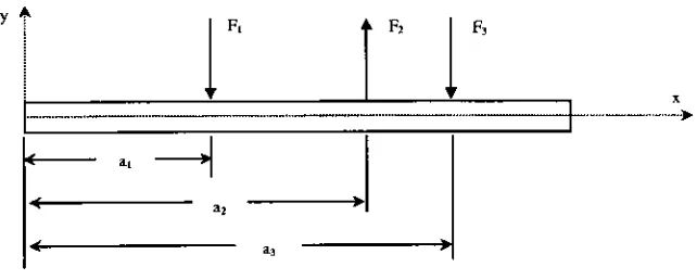
(see Fig. 2.1).
A
i
F,
iiF2
i
F3
r
ai
a2
a3
-Figure 2.1 Three Transverse Point Loads
(at
distances
a1? a2
and
a3
respectively)
While
three-dimensional
modeling
would
more
accurately
represent
true
labial
configurations,
loads
and
deflections
were considered
only in
two
dimensions
to
further
simplify
the
problem.
The 2D
approach
used
here
can
be
expanded
into
three
dimensions
[image:20.566.120.441.349.478.2]Axial
loading
is
not considered
here,
though
further study
with
combined
loading
scenarios
is
warranted.
2.2.2
Simplification
of
Possible
Constraints
Standard beam
theories
exist
for beams
that
are
rigidly
clamped,
simply
supported,
cantilevered,
or
bound
by
some combination of
those
constraints.
Because
of
the
bUateral
symmetry
of
the
mouth about
its
mid-span, the
same constraints were chosen
for
the
left
end
of
the
beam
model
that
were
chosen
for
the
right
end;
no actual mouth
has lips
that
are
perfectly
symmetric
in
shape or
flexibility,
but for
the
purposes of
this
study
they
are
assumed so.
The
cantilevered condition was not considered
because
of
the
non-symmetric
nature of
the
deflection
curve which
did
not
have
an anatomic
justification. For
this study,
symmetric models of
rigidly
clamped and
simply
supported
beams
were
considered.
2.2.3
Simplification
of
Possible Beam
Shapes
Modifying
a
beam's
cross sectional shape affects
its
moment of
inertia,
/. This in
turn
affects
the
deflection
calculations.
Beams
of
circular cross-section were weU suited
for
this
study
since
radius,
r,
is
the
only
variable
needed
to
calculate
/ (see Eq. 2.1). The
moment of
inertia
for
square and semi-circular cross-sectioned
beams
also
rely only
on
a single
variable, though
it is
easier
to
define
the
centerUne and outside edges of a circular cross-section
beam
than
for
one
that
is
not
axisymmetric.
Further,
beams
with
straight centroidal axes were used
in
this
study.
Under
these constraints,
two types
of
beams
were
considered: cylindrical
beams
of constant
radius
(prismatic)
and cylindrical
beams
whose radU varied
along
the
length
of
the
beams
(tapered).
Prismatic beams have
constant radU and
thus
constant moments of
inertia;
they
were
defined
as
Type 1 beams. Tapered beams have
varied
radU and
thus
varied
/
and were
defined
as
Type
2. The
moment of
inertia
of a cylinder
is
directly
related
to
its
radius.
The
relation
between
the
moment of
inertia
of a cylinder and
its
radius provided
the
first
geometric parameter
for
consideration
(see
Sec.
3.2.3).
A
prismatic
beam
of circular
cross-section
(Type
1)
and
radius,
r,
has
a constant area
moment of
inertia, /,
given
by
Eq. 2.1 [Beer
and
Johnston 1992]:
I
=L=Iy=7rcr4
(2.1)
4
For
a
tapered
beam,
the
radius and
the
area moment of
inertia
are
both
functions
of
length,
r(x)
and
I(x). Since
the
derivations
of
the
deflection
equations require several
integrations,
a
varied
area moment of
inertia,
I(x),
with
a profile
tapered
at
both
ends
that
was
relatively
easy
to
integrate
was
devised (Eq.
2.2).
Ia
and
Ib
are parameters
that
can
be
adjusted
to
control
the
profile of
the
area moment of
inertia.
Assuming
that
each circular cross-section of
the tapered
beam
has
the
same
local relationship
between
the
radius and
the
area moment of
inertia,
the radius,
r(x),
was
defined
as a
function
ofl(x)
(Eq. 2.3).
r(x)
v
K
J
(2.3)
The
parameters
that
aUow modification of
the
way
radius changes
along
the
length
of
the
beam
are
Ia
and
h. This
results
in
a
beam
as shown
in Fig. 2.2.
Figure 2.2
Cylindrical Beam
with
Varied Radius
2.2.4
Other
Assumptions
Standard Euler-BernoulU beam
theory
assumes
that
plane sections remain plane
during
bending
[Fenner
1989]. In
addition
to this
and other standard assumptions
for
these
beam
deflection
theories
[Fenner
1989,
p.
253],
the
foUowing
assumptions
have been
made
for
this
study:
Effects
of
the
teeth
and
tongue
are not
to
be
considered
in
the
geometric constraints of
the
problem.
The
teeth
and
tongue
are
part of
the
general
make-up
of
the
mouth and account
for
a great
deal
of
its
appearance.
The
Ups
can act
independently
from
the teeth
and
tongue,
so
to
achieve
the
largest
possible range of motions
for
the
face
as a
whole,
models
for
each
component can
be developed
independently
and
brought
together
assuming
appropriate
superposition
relations could
be
established a priori.
Since
the
actions of
the teeth
and
tongue
effect
the
behavior
and motion of
the
Ups,
there
is
a
danger
of
deriving
impossible
facial
configurations.
This
can
be
avoided
by linking
the
models
-letting
them
share certain
common
parameters.
This
would
then
cause
the
Ups
to
move a certain
way if
the teeth
are
moving
a certain way.
SmaU deflections
and smaU angular
displacements
are assumed
for
the
beam
to
faciUtate
calculation
of
the
displacement
equations.
While
actual
Up
deflections
and angular
displacements
are
large
and would
seem
to
invalidate
these
two assumptions,
the
basic
curve
shapes can stiU
be found. Once
the
shape profile
is
defined,
a
scaling
parameter
could
be
used
to
adjust
the
magnitude of
the
deflections.
The
principal
of
superposition
is
used
in
this
study
to
add
the
effects of more
than
one
load
to
the
beam. In
order
for
this
technique
to
be
vaUd,
each
deflection
must
be
linearly
related
to
the
load
that
causes
it
and
the
deformation resulting from any
given
load
must
be
small
and
not affect
the
conditions of appUcation of
the
other
loads. Due
to
the
relative
simpUcity
of
the
deflection
equations
for
materials
in
their
elastic ranges
(as
opposed
to
deflections in
the
plastic
range),
aU
beams
studied are assumed
to
be
flexing
elasticaUy.
The
elastic
assumption
and
the
small
deflection
assumption
cover
both
criteria of
the
principal of
superposition.
2.2.5
Summary
of
Beam
Cases
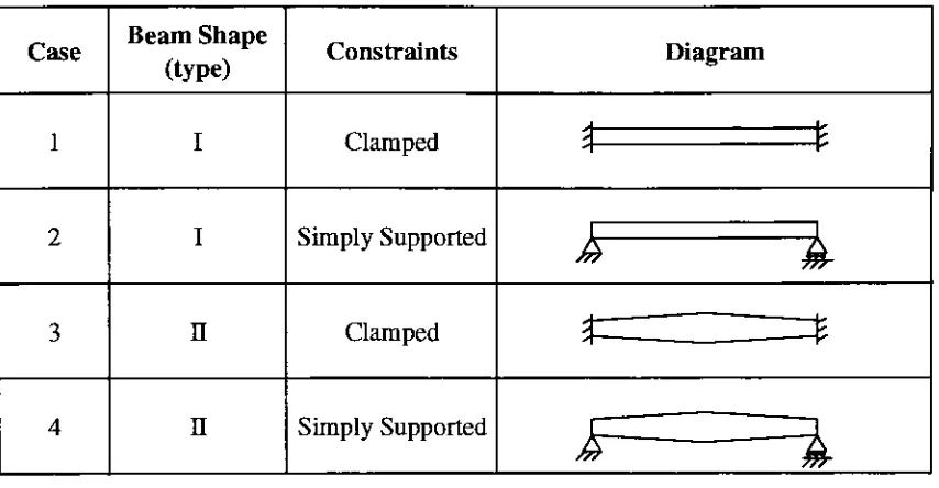
The four beam
types
are
summarized
in Table 2.1.
Case
Beam
Shape
(type)
Constraints
Diagram
1
I
Clamped
* ^2
I
Simply
Supported
1
1
i
A
3
n
Clamped
3=
=*
4
n
Simply
Supported
s=%
Table
2.1 Beam
Configurations
2.3
Calculation
of
Deflections
With
the
beam
geometries and constraints
defined,
deflection
equations were
determined for
each of
four beam/constraint
cases.
Due
to the
bUateral symmetry
of
Ups,
beams
with
different
end constraints were not
investigated. The
ends of
the
beam
were
thus
both simply
supported or
both
clamped.
The four beam
cases are
described
in
sections
2.3.1
through
2.3.4.
AU
cases possess similar
coordinate axes and a single point
load,
F,
acting
on
the
beam in
the
-y
direction
at a
distance
x
=a
from
the
origin.
The
effects of multiple
loads
were examined
using
superposition
-where
the
deflections
of
the
system
caused
by
each
individual load
were calculated and
then
summed
to
yield
the total
deflection
solution.
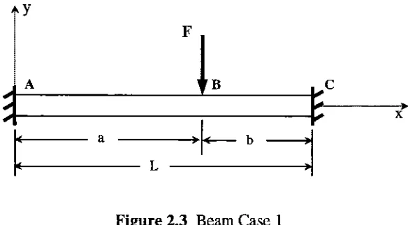
[image:25.566.61.488.131.353.2]2.3.1
Case 1
Beam
Case
1 is depicted in Figure 2.3.
*y
l
B
Figure
2.3 Beam Case 1
Shigley
and
Mischke
[1989]
provides
the
deflection
equations,
included here
as
Eq. 2.4
and
Eq.
2.5,
for
a point-loaded
beam
with
clamped
boundaries (Case 1). Eq. 2.4 describes
the
deflection
curve
for
the
beam from
the
origin
(jc
=0)
to the
point of
loading
(jc
=a).
Eq. 2.5
describes
the
deflection
curve
from
the
point of
loading
to the
end at
x
=L.
FOX
r i 72 r2i6EIL
^ni^2-2-2^
(2.4)
(2.5)
In
order
to
faciUtate
the
use of
these equations,
singularity
functions
were used
to
combine
them
both into
a single
deflection
equation,
Eq.
2.6.
y(x)
=+
(2.6)
where
the
singularity function
is
defined in Fenner
[1989]
as
foUows:
f(x)
=(x-aY
=\
J
N
'
\{x-a)n
x<a
x>a
(2.7)
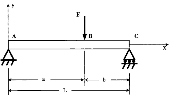
[image:26.566.141.433.163.324.2]2.3.2
Case 2
Beam Case 2 is depicted in Fig. 2.4.
*y
&
y*
L
[image:27.566.142.439.153.338.2]%
Figure 2.4 Beam Case 2
Shigley
and
Mischke
[1989]
again
provide
two
deflection
equations:
one
for
x
<a
and
another
for
x
>a.
These
equations used
as-is,
however,
are valid
only for
a
>
b
(unless
discontinuity
functions
are
appropriately
used).
GeneraUy,
for
a
<
b
one must
take
advantage of
symmetry
and examine
the
beam from
the
other
end.
Both
equations converge
to the
same solution
for
a
=b. In
this case,
however,
it is
more advantageous
to
use an
alternate
formulation
that
provides a single equation.
Fenner
[1989]
begins
with
the
bending
moment
distribution,
M(x),
and
incorporates it into
the
moment-curvature
relationship
shown
inEq.
2.8.
d2y
M(x)
dx1
/(jc)
(2.8)
Simplified for
the
constant
area moment of
inertia
(/)
case, this
equation can
be
written:
EIdjL=
M(x)
(2.9)
dx
Integrating
Eq. 2.9
twice
with respect
to
jc,
yields y(x).
Using
this technique
for
a
simply
supported
beam
simUar
to
that
of
Case
2,
Fenner
[1989]
derives
the
foUowing
deflection
equation:
y(x)
=EI
Fbx3F,
X3Fb.Tl
,2x(x-a)
+
(Zf-Zr);
6L
6X'
6L
(2.10)
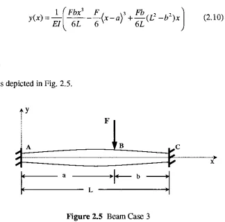
2.3.3
Case 3
Beam
Case 3 is depicted in Fig. 2.5.
Figure
2.5 Beam
Case
3
The
technique
used
to
derive
the
deflection
equation
for
this
beam
is
simUar
to the
one used
by
Fenner
[1989]
as noted
in Case 2. The difference Ues in
boundary
conditions and
that the
beam has
an area
moment of
inertia, /,
which
is
no
longer
constant
but
a
function
of
jc
(Eq.
2.3). This
compUcates
the
integration
needed
to
determine
the
deflection
equation,
but
not
prohibitively
so.
Substituting
the
bending
moment
distribution
and
the
expression
for
I(x)
into
the
moment-curvature
relation
in Eq. 2.8
results
in
the
deflection
equation.
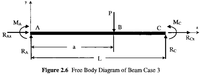
[image:28.566.128.452.182.502.2]A free
body
diagram
(FBD)
of
this
beam is
shown
in Fig.2.6:
y
a
R
MA
Ax
\^
Ra
P
A
uBC
<
a
?i
<
L
>.5
Mc
X
>
Rex
Re
Figure
2.6 Free
Body
Diagram
of
Beam
Case 3
Expressed using
a
singularity
function,
the
shear
force distribution in
the
beam
is:
V(x)
=RA-P(x-a)
(2.11)
Given
that
the
shear
force
at
any
position
along
a
beam is
equal
to
the
slope of
the
bending
moment
distribution [Fenner
1989],
M(x)
can
be
expressed as
in Eq. 2.9 (also
see
Appendix
A
on
integrating
singularity
functions)
such
that:
M(x)
=RAx-P(x-a)1
+
C3
(2.12)
From
this
equation
and
the
FBD
in Fig.
2.6,
it is
noted
that
MA
=M(0)
=C3.
So Eq. 2.8 becomes:
d2y
=1
(RAx-P{x-a)1+C3)
dx2
E
IA
(2.13)
(x-L/J
+
l.
or,
simplified:
IAE^
=(RAx-P(x-a)l+C3)
x-L/2)+Ib
(2.14)
Integrating
once
with
respect
to
jc
over
the
interval
x
=0
to
x
=L
gives an expression
for
the
slope of
the
beam along
its
length:
[image:29.566.86.478.114.261.2](2.15)
"A
IAE^-=(IAE)C1
dx
+
(L(x-jty
+
iBx+^y)c3
+
(-
t(*-f
)2<*
-+
i(*
-tXx
-4
-M*
-aY
-t'*<*
-a)2)p
Integrating
again with respect
to
jc
over
the
interval
jc
=0
to
x
=L
gives an expression
for
the
deflection
of
the
beam along its length (appendix A
provides a
detaded
example of
this
type
of
integration):
IAEy(x)
=(lAEx)C1
+
(IAE)C2
+
fe-(*
-i)4
-(*
)4
+
IV2+
i(i)3^3
^{-^-^{x-aY+^x-Wx-aY-^x-af-^I^x-aYy
By
applying
the
boundary
conditions
for
clamped-clamped
beam,
values
for
the
constants
Q,
C2, C3,
and
RA
are
determined. At both
the
left-
and right-hand
supports,
the
slope
and
the
deflection
of
the
beam
are
zero, thus:
y(0)
=y(L)
=0
(2.17)
and:
^
=0
atx
=0,L
(2.18)
dx
Evaluating
Eq. 2.16 using
the
boundary
conditions at x
=0
directly
results
in
the
determination
of
Ci
=C2
=0.
Applying
the
boundary
conditions at
x
=L
creates
two
equations of
the
form
ocC3
+
PRa
=yP,
where
the
coefficients
a,
p\
and
y
are
defined
as
foUows:
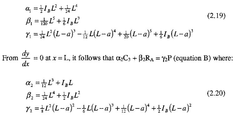
From
y(L)
=0,
it foUows
that
OC1C3
+
PiRA
=TiP
(equation
A)
where:
"l
21B1^~
24-^
(2.19)
R
=+T
I3Pi
120-^ ^61BL^7l=j;L2{L-ay
-L{L-aY
+Jz{L-a)5
+iIB{L-af
dy
From
=0
at
jc
=L,
it foUows
that a2C3
+
P2RA
=Y2P
(equation
B)
where:
dx
a2=L3+IBL
R
=J-L4+J-/L2
lJ2
It,1-'~
2lBL-1
(2.20)
72=|L2(L-a)2-iL(L-a)3+1L(L-)4+i/s(L-)2
Solving
equations
A
and
B (see Appendix
B)
results
in
expressions
for
C3
and
Ra
in
terms
of
the
a,
p\
and
y's
in Eq. 2.19
and
Eq. 2.20.
axp2
-ar2#
{a{Yi-cc27x)P
ViPi-ViPi
RA
=(2.21)
(2.22)
2.3.4
Case 4
Beam
Case 4 is depicted in Fig. 2.7.
Ay
1
B
777"
<
b
>
[image:31.566.91.468.75.267.2]L
Figure 2.7 Case 4
Equations
(2.11)
through
(2.16)
are stiU vaUd
for
the
deflection
of
this type
of
beam,
however
the
boundary
conditions
have
changed so
the
constants
d,
C2, C3,
and
Ra
are
different.
Since
the
beam is simply
supported,
no moments exist at
the
ends
jc
=0
and
x=L,
and
using
Eq. 2.12
with
these
conditions yields:
M(x)
=RAx-P(x-a)l+C3
(2.12)
M(0)
=C3
.-.
C3
=0
(2.23)
M(L)=RAL-P(L-a)
+
C3
P(L-a)
(2-24)
.:RA
=
There
is
also no
deflection
at
the
ends x
=0
and x
=L
Solving
Eq.
2. 16 for
x
=0
directly
results
in
C2
=0. At
x
=L,
Eq. 2.16
yields
Eq. 2.25:
0
=(/AJEL)C1
+
(^IBL2+^yL)c3
(225)
(-l(K)2(L-a)3+|(K)(L-fl)4-^(L-a)5-l/(L-a)3)p
+ 1
+
1
Using
equations
2.23
and
2.24 in 2.25
yields
d:
0
={lAEL)C1+/]1RA+y1P
:.Cl=^{-PxRA
+
riP)
<2-26>
IBEL
where
Pi,
yi,
and
ai
are
as
in Eq. 2.19.
Microsoft Excel
was used
to
generate
the
Up
curves
from
the
respective
deflection
equation
for
the
beam/load
case
being
considered.
Visual Basic
modules were written
to
execute
the
custom
functions
-to
graphicaUy
display
the
functions just derived.
2.4
Verifying
Type 2 Beam Models
The deflection
equations used
for
aU
Case 1
and
Case 2
scenarios
(Type 1
beams)
were
assumed
to
be
vaUd since
they
are
simply
combinations of equations
directly
from
Shigley
and
Mischke
[1989]
(see Sec. 2.3.1
and
2.3.2). The
equations
for
the
beams
with varied
cross-sections,
however,
are adaptations of accepted equations
and,
as
such,
were
verified
before continuing
with
the
analysis.
An
average area moment of
inertia, Iavg,
was
determined
by integrating
the
function
I(x)
(see Appendix C). This
was used as
the
constant value of
the
moment
of
inertia for
the
prismatic
(Type
1)
beams. To
observe
the
convergence
of
the
different beam
models, the
moment of
inertia
parameters
I
a
and
h
were
adjusted
to
let
I(x)
be essentiaUy
constant
along
the
length
of
the
beam. With
an
essentiaUy
constant
I(x),
the
deflection
curve should
converge on
the
constant
/
solution.
ArbitrarUy
setting
the
parameters as
foUows sufficiently
"immobilizes"
the
variable area moment of
inertia:
IA
=5 E 12
mm4
and
IB
=5E6
mm2.
3.
Testing
Approach
3.1
Beam
Shape
Table 2. 1
outlines
the
four beam
configurations
that
were studied.
Deflection
equations
for
those
cases are as noted
in
sections
2.3.1
through
2.3.4.
3.2
Loading
Scenarios
Loading
scenarios
(or
trials)
were
run
on
the
four
Up
models
to
examine
the
possible shapes
they
could
generate.
Single
transverse
point
loads
were appUed
in
the
modeL
The
effects of
multiple
loads
was
determined
by
adding
or
"superposing"the
individual
effects
from
each
load
under
the
assumption
of
linearity
(see
Sec. 2.2.4).
A
given
beam
was
arbitrarUy divided into 10
equi-spaced segments
(11
nodes,
including
the
two
end points).
A
force
of
100
units
was appUed
to the
first
node and
the
resulting
deflection
was noted.
The
force
was
then
moved
to
each of
the
other nodes
(excluding
the
end
nodes)
and
the
deflection
computation
repeated.
3.3
Comparison Criteria
By increasing
the
number
of
loads
on
the
beam,
most
any
contour can
be
achieved,
though
the
goal
here is
to
determine
if
beam-bending
theory
lends
itself
to
a simple modeL
As
the
number of
loads necessary
to
achieve
the
appropriate shape
increases,
the
usefulness of
this
technique
rapidly diminishes. The
flexibiUty
and
simpUcity
of each model were compared
with
the
others
in
order
to
determine if
sufficient
differences
exist
between
them
and
to
see
if
one model stood out
from
the
rest as
the
most efficient.
This
was
done
by
comparing
modeled
Up
curves with actual
human
Up
curves.
Actual human
Up
shapes
were
documented
for
various
facial
expressions obtained
from
photographs of
the
author.
The
centerline of
each
Up
image
was
determined
and
defined
as
the
actual
Up
curve.
Each
of
the
four beam
models
was
tested
with
different
numbers of
loads in
an attempt
to
successfuUy
match
the
shape of
its
respective actual
Up
curve.
Each
modeled curve was superimposed over a plot of
its
respective actual
Up
curve and a statistical
R2value
was
determined
to
show
the
goodness
of
the
fit (see Eq. 3.1).
/?z=l
2 .SSE
SST
SSE^U-Y,]
(3.1)
SST
=%?
-iforf
A
Yi
represents
Up
deflections
taken
from
the
digitized
photographs,
Yi
represents
Up
deflections
calculated
using
a
model
and
n
represents
the
total
number of
data
points.
R
is
defined
as
Pearson's Product-Moment Correlation
Coefficient
[Sheskin
1997]
and
provides a normaUzed measure of
the
goodness of
the
fit.
SSE
is
the
Sum
of
the
Squared
Errors
and
SST is
the
Sum
of
Squared Terms.
4.
Analyses
4.1
Lip-Curve
Data Collection
Photographs
were
taken
of
the
author's
Ups (see
subject
data in Appendix
E)
in
as
many
positions
as
he
could achieve
using
only
facial
muscles.
One
such photograph
is
shown
in
Photo. 4.1.
ManuaUy
pulling
the
Ups into different
positions was not permitted
in
this
study
as
those
configurations are not part of natural speech and
facial
expressions.
Photograph
4.1
Scanned
Image,
Photo
24
A
total
of
25 different
mouth expressions were
achieved; the
shape of each
Up
within each
mouth
image
was
documented
by
measuring
the
Up's displacement from
a mouth centerline
defined
by
a
line
segment
connecting
the
corners of
the
mouth.
For
the
purposes of
this
study, the
actual
lip
curve
is defined
as
the
curve
halfway
between
the
upper and
lower
visible
boundaries
on each
Up
(indicated
by
the
dotted line in Photo.
4.2).
Photograph
4.2 Photo 24
withLip
Centerline
(dashed)
and
Actual
Lip
Curves
(dotted)
Shown
Since
each photographed mouth configuration
has
two
visible
Ups,
50 deflection
curves were
attained.
AU
digitized
Up
measurements can
be found in Appendix D.
To correctly determine
the
actual size of
the
Ups
within
each
photograph,
a metric ruler was
placed
just
below
the
mouth
in every
shot
(see Photo. 4. 1). A 10
mm
line
segment was
compared
to the
length
of
the
image
of a
10
mm
segment,
LP,
on
the
ruler
in
the
picture.
The
scale
factor,
S,
therefore
is
defined
as:
S=
(4.1)
AU
Up
deflections
were multipUed
by
this
scale
factor
before continuing
with
any
analyses
or
comparisons.
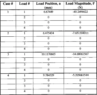
4.2
Model
Comparisons
Two
of
the
25
sample mouth expressions
(thus four
Up
images
-two
from
photo
02
and
two
from
photo
24)
were
taken
and used
for
comparison
trials
with
the
various
beam
cases
(Photo.
4.3
and
Photo.
4.1).
Photograph
4.3
Scanned
Image,
Photo 02
The
position
and magnitude of
the
loads acting
on
each
beam
model were adjusted
to
match
modeled
deflections
as
closely
as possible with actual
deflection
curves.
Microsoft
Excel's
optimization routine
within
its
solver
(see Appendix
E)
was used
to
minimize
the
sum of
the
squares of
the
differences between
actual and
beam
model-predicted curves
by
adjusting
magnitude and
position
of point
loads
within
the
beam
modeL
Comparisons
were carried out
for beam
models with
one,
two, three,
and
four independent
loads.
For
the
Up
models
relating
to
photo
24,
the
leng