Exploring the ingredients required to successfully model the placement, generation, and evolution of ice streams in the British-Irish Ice Sheet

This is a repository copy of

Exploring the ingredients required to successfully model the

placement, generation, and evolution of ice streams in the British-Irish Ice Sheet

.

White Rose Research Online URL for this paper:

http://eprints.whiterose.ac.uk/150398/

Version: Published Version

Article:

Gandy, N., Gregoire, L., Ely, J. orcid.org/0000-0003-4007-1500 et al. (3 more authors)

(2019) Exploring the ingredients required to successfully model the placement, generation,

and evolution of ice streams in the British-Irish Ice Sheet. Quaternary Science Reviews,

223. ISSN 0277-3791

https://doi.org/10.1016/j.quascirev.2019.105915

[email protected]

https://eprints.whiterose.ac.uk/

Reuse

This article is distributed under the terms of the Creative Commons Attribution (CC BY) licence. This licence

allows you to distribute, remix, tweak, and build upon the work, even commercially, as long as you credit the

authors for the original work. More information and the full terms of the licence here:

https://creativecommons.org/licenses/

Takedown

If you consider content in White Rose Research Online to be in breach of UK law, please notify us by

Exploring the ingredients required to successfully model the

placement, generation, and evolution of ice streams in the British-Irish

Ice Sheet

Niall Gandy

_{, Lauren J. Gregoire}

_{, Jeremy C. Ely}

_{, Stephen L. Cornford}

_,

Christopher D. Clark

, David M. Hodgson

a

School of Earth and Environment, The University of Leeds, Leeds, LS2 9JT, UK b_{Department of Geography, The University of Sheffield, Sheffield, S10 2TN, UK} c_{Department of Geography, Swansea University, Swansea, SA2 8PP, UK}

a r t i c l e

i n f o

Article history:

Received 4 June 2019 Received in revised form 2 September 2019 Accepted 3 September 2019 Available online xxx

Keywords:

British-Irish Ice Sheet Ice streams Basal hydrology Ice sheet modelling Model-data intercomparison

a b s t r a c t

Ice stream evolution is a major uncertainty in projections of the future of the Greenland and Antarctic Ice sheets. Accurate simulation of ice stream evolution requires an understanding of a number of “ in-gredients”that control the location and behaviour of ice streamflow. Here, we test the influence of geothermal heatflux, grid resolution, and bed hydrology on simulated ice streaming. The palaeo-record provides snapshots of ice stream evolution, with a particularly well constrained ice sheet being the British-Irish Ice Sheet (BIIS). We implement a new basal sliding scheme coupled with thermo-mechanics into the BISICLES ice sheet model, to simulate the evolution of the BIIS ice streams. Wefind that the simulated location and spacing of ice streams matches well with the empirical reconstructions of ice streamflow in terms of position and direction when simple bed hydrology is included. We show that the new basal sliding scheme allows the accurate simulation for the majority of BIIS ice streams. The extensive empirical record of the BIIS has allowed the testing of model inputs, and has helped demonstrate the skill of the ice sheet model in simulating the evolution of the location, spacing, and migration of ice streams through millennia. Simulated ice streams also prompt new empirical mapping of features indicative of streaming in the North Channel region. Ice sheet model development has allowed accurate simulation of the palaeo record, and allows for improved modelling of future ice stream behaviour.

©2019 The Authors. Published by Elsevier Ltd. This is an open access article under the CC BY license (http://creativecommons.org/licenses/by/4.0/).

1. Introduction

Ice streams dominate discharge in our contemporary ice sheets,

routing ice from the ice sheet interior to the margins (Bennett,

2003). Ice streams account for 90% of the discharge of the

Antarc-tic Ice Sheet (Bamber et al., 2000), and a number of ice streams have

been identified as key points of vulnerability for the future

evolu-tion of the Antarctic (e.g.Favier et al., 2014;Nias et al., 2016;Waibel,

2017) and Greenland (e.g.Joughin et al., 2008;Gillet-Chaulet et al.,

2012; Hogg et al., 2016) ice sheets. Given the importance of ice stream dynamics on ice sheet evolution, understanding stream evolution is crucial to elucidating the future of the Antarctic and

Greenland Ice Sheets.

Ice stream behaviour within advancing, stable, and retreating ice sheets remains unclear, and accurate simulation of these

pro-cesses is a key challenge of glaciology (Hindmarsh, 2018p.625).

Observations from contemporary ice sheets and reconstructions of palaeo ice sheets show that ice streams are spatially and temporally

variable (Conway et al., 2002;Dowdeswell et al., 2006;Stokes et al.,

2009;O Cofaigh et al., 2010 ;Margold et al., 2015), but the causes of

this variability remain poorly understood (Siegert et al., 2004;

Horgan and Anandakrishnan, 2006; Peters et al., 2006).

Simula-tions of contemporary ice sheets typically achieve a close _fit to

observed surface speeds using data assimilation techniques that

tune ice sheet parameters such as effective drag (Gillet-Chaulet

et al., 2012; Morlighem et al., 2013; Arthern et al., 2015; Gong et al., 2017). While this achieves a close match to observations over decadal timescales, it does not account for long-term changes

*Corresponding author.

E-mail address:[email protected](N. Gandy).

Contents lists available atScienceDirect

Quaternary Science Reviews

j o u r n a l h o m e p a g e :w w w . e l s e v i e r . c o m / l o c a t e / q u a s c i r e v

https://doi.org/10.1016/j.quascirev.2019.105915

to bed hydrology, meaning it is expected that such ice sheet sim-ulations will diverge considerably from reality, even given a perfect

climate forcing (van der Veen, 1999). And, when modelling regions

without present-day ice cover, there are insuf_ficient observations,

rendering these data-hungry methods entirely useless. Studies of palaeo ice sheets use a variety of methods to represent basal

fric-tion, including relationships with basal elevation (Martin et al.,

2011; Seguinot et al., 2016), sediment thickness (Peltier, 2004;

Gregoire et al., 2012,2015), or idealised bed classifications (Boulton and Hagdorn, 2006;Gandy et al., 2018). These representations use proxies of bed friction, and the do not capture the evolution of basal hydrology over a glacial cycle.

Improved simulations of ice streams require a representation of the physical mechanisms of ice streaming. Ice streams achieve their enhanced velocity through basal processes, and typically occur over areas of low bed friction. The friction at the bed of an ice stream is likely to evolve due to a number of processes that operate at dif-ference timescales. Over long (millennial) timescales, glacial erosion and deposition can alter the force balance of the bed. Erosion may change the shape of basal obstacles, altering the form

drag between the ice and the bed (Schoof, 2002). Sediment

depo-sition may also mask smaller basal obstacles, and change regions

where sediment deformation occurs (Bingham et al., 2017;Davies

et al., 2018).

The most rapid change to basal friction can occur due to

sub-glacial hydrology, as differences in water routing, subsub-glacial_floods,

and supra-glacial water inputs can all dramatically alter the vol-umes and spatial patterns of water at the bed over short (diurnal to

decadal) timescale (Nye, 1976; Smith et al., 2007; Hewitt and

Fowler, 2008). Detailed kilometre-scale patterning of basal shear stress under ice streams, inferred through observations and in-versions, has been deduced for the Antarctic and Greenland ice

sheets (Inversion, 2013;Sergienko et al., 2014), who used

mathe-matical modelling to explain them by coupling water and iceflow.

Corresponding geomorphological features in the palaeo-record

have been observed (Stokes et al., 2016). The thermal regime of

the ice, determined by basal friction, geothermal heatfluxes, and

englacial ice temperatures, can also influence subglacial hydrology

and sliding rates (Payne, 1995). Basal water pressure at the

Whil-lans Ice Stream, West Antarctica, is close to the ice floatation

pressure (Engelhardt and Kamb, 1997;Kamb, 2013), and increased

surface melting has been linked to increased ice velocity of the

Greenland ice sheet (Zwally et al., 2002), both suggesting that

subglacial water availability and routing is a key control of ice streaming. Subglacial meltwater can promote ice streaming by saturating basal sediments, and thus encouraging sediment defor-mation and sliding across bedrock. However, the inaccessibility of basal environments is an obstacle to more robustly describing and

understanding subglacial processes (Hewitt, 2011). The

represen-tation of ice streaming and subglacial hydrology has been a key area for development for numerical ice sheet models of varying

complexity (Greve, 1997;Bougamont et al., 2011;Bueler and van

Pelt, 2015). Due to the uncertainty of basal processes simulations usually ignore some processes and idealise others. The palaeo re-cord offers the chance to test whether ignoring and idealising some basal processes is appropriate.

Here, we aim to introduce an idealised representation of sub-glacial hydrology to simulate the ice stream and ice sheet evolution of the British-Irish Ice Sheet (BIIS). To meet this aim, we address the following objectives: 1) we describe new development of the BISICLES ice sheet model; 2) we employ the BIIS palaeo archive of ice stream locations to test the skill of the ice sheet model in simulating ice stream advance and retreat over the millennial timescale; 3) we discuss the ingredients required to accurately model ice streams of the BIIS.

1.1. Background

1.1.1. Ice stream modelling

Accurately simulating ice streams within an ice sheet model is a

key concern because of the large influence of ice streams on ice

sheet behaviour and stability. Grounded ice streams with marine

margins have been identi_fied as points of vulnerability in the future

evolution of ice sheets, in particular the West Antarctic Ice Sheet, because ice streams on a retrograde bed slope are prone to Marine

Ice Sheet Instability (MISI) (Schoof, 2007). Theoretical

in-vestigations of MISI have almost exclusively assumed an ice sheet sliding on bedrock with a viscous power-law relationship between

velocity and stress (Hindmarsh and Meur, 2001; Schoof, 2007;

Gladstone et al., 2018). However, there is some evidence that a Coulomb friction approach may be applicable close to the

grounding line (Iverson et al., 1998;Schoof, 2006). Recent work has

shown that a combined Coulomb and viscous power-law approach

changes ice sheet profiles, and causes the stable grounding line

position to be in shallower water than a plastic power-law only

approach (Tsai et al., 2015).

Models of contemporary ice sheets have achieved a closefit to

the observed ice surface velocities (Morlighem et al., 2013), using

an optimization technique to determine subglacial friction pa-rameters to match surface velocities. In effect, a spatially varying basal friction parameter obtained accounts for unknown bed and englacial properties. Simulations of contemporary Greenland (e.g.

Lee et al., 2015) and Antarctica (e.g.Favier et al., 2014;Cornford et al., 2015) are a strong match for the empirical evidence, and may well be a suitable starting point for decadal to centennial future projections, but typically do not allow the basal friction parameters to vary through time. Therefore, centennial to millen-nial future projections will require ice stream modelling that is

capable of ice stream evolution (Aschwanden et al., 2013).

Currently, ice sheet models have success modelling ice streams through a theory of thermomechanical instability, where fast ice

flow is allowed once the ice has reached the basal pressure melting

point (Hindmarsh, 2018). This spontaneous generation of ice

streams has been modelled given a flat bed (Payne and

Dongelmans, 1997), with regularly spaced ice streams forming

due to thermomechanical instabilities of ice sheetflow.Hindmarsh

(2009)showed the importance of simulating both horizontal

lon-gitudinal and lateral stresses e membrane stresses - when

modelling ice stream generation. Idealised experiments that incorporate a representation of subglacial hydrology demonstrate

that ice stream formation can be a response to basal water_flow

rather than ice sheet thermomechanics (Kyrke-Smith et al., 2013).

Applying ice stream modelling to contemporary and palaeo ice sheets is challenging owing to the complexity and scale of real ice sheet beds. The simulation of evolving ice streams has been

un-dertaken in a number of palaeo (e.gHubbard et al., 2009;Jamieson

et al., 2012;Patton et al., 2016;Gandy et al., 2018;Seguinot et al.,

2018) and contemporary (Aschwanden et al., 2013,2019) studies.

Despite progress in simulating ice streams, the skill of models to generate ice streams that evolve over the millennial time-scale has not been adequately tested against the empirical palaeo record.

1.1.2. Palaeo ice streams

Whilst contemporary observations can produce detailed infor-mation on current ice sheets, they do not record the multi-decadal, centennial and millennial variability of the ice stream activity and position. Limited contemporary ice stream evolution has been observed, with the most studied example being the change in discharge of ice streams along the Siple Coast of West Antarctica (Retzlaff and Bentley, 1993; Conway et al., 2002). Therefore, the history of contemporary ice sheet observation is not yet long

N. Gandy et al. / Quaternary Science Reviews 223 (2019) 105915

enough to observe the results of signi_ficant margin changes, ice temperature evolution, or basal friction evolution. The record from palaeo ice sheets offers an opportunity to test methods for modelling ice streams against an archive spanning millennia, rather than a contemporary snap-shot of ice streaming. The imprint of palaeo ice streams can be determined from a set of well-established diagnostic geomorphological and sedimentological signatures (Stokes and Clark, 1999; Clark and Stokes, 2001; Margold et al.,

2015), such as MSGL (Clark, 1993), Trough Mouth Fans (Vorren

and Laberg, 1997), and subglacial bedform convergence (Everest et al., 2005). Increased mapping of palaeo-ice stream tracks (Hughes et al., 2014;Margold et al., 2015) offers a record of ice stream and ice sheet evolution over millennia. Efforts to both

relatively and absolutely dateflowsets of palaeo ice sheets have

been extensive (Greenwood and Clark, 2009;Margold et al., 2015,

2018;Hughes et al., 2016;Small et al., 2017), resulting in a wealth of palaeo ice sheet mapping.

Whilst the palaeo-record offers a test-bed for ice stream modelling, the modelling of palaeo-ice stream location and evolu-tion can also inform empirical reconstrucevolu-tion efforts. The landform record is increasingly well documented, but will always be an

incomplete record of ice sheet behaviour. A model that has suffi

-cient skill to simulate empirically well constrained ice streams may highlight potential locations of unmapped ice streams. In this

manner, the model benefits from the extensive testing opportunity

provided by the palaeo record, and in turn models can also help target work to extend the empirical record. This creates a symbiotic

relationship between numerical modelling and empirical

reconstructions.

1.1.3. The British-Irish Ice Sheet

Testing an ice sheet model against the palaeo record requires

confidence in the empirical data. The British-Irish Ice Sheet (BIIS)

arguably offers the most complete archive of data constraining the behaviour of an ice sheet and several ice streams over millennia. Mapping of glacial features has greatly expanded since the advent

of remote sensing techniques (Clark et al., 2004;Smith et al., 2006),

complementing signi_ficant chronology work (Hughes et al., 2011).

Recently, a wealth of offshore data collection has considerably

expanded the palaeo archive of the BIIS (e.gBradwell et al., 2008b;

OCofaigh et al., 2016;Dove et al., 2017). Empirical work spanning decades has cumulatively led to an extensive palaeo archive for the

BIIS (Clark et al., 2018).

Using this wealth of empirical evidence, numerous ice stream locations have been reconstructed both onshore and offshore with

evidence from subglacial lineations (Hughes et al., 2014), trough

mouth fans (Bradwell et al., 2008b), and topographic troughs.

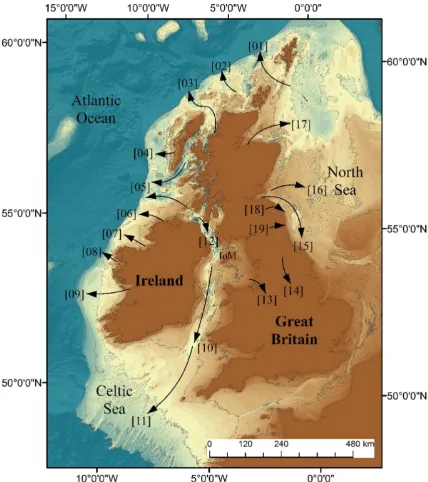
Reconstruction of large ice streams offshore are numbered onFig. 1

andTable 1, and include the Rona [01] (Bradwell et al., 2008b), the

Foula [02] (Bradwell et al., 2008b), the Minch [03] (Stoker and

Bradwell, 2005), the Barra Fan [05] (Finlayson et al., 2014), the

Irish Sea [10] (Chiverrell et al., 2013), the Celtic Sea [11] (Scourse

et al., 2009), the North Sea Lobe [15] (Dove et al., 2017), the Firth

of Forth [16] (Hughes et al., 2014), and the Moray Firth [17] (Merritt

et al., 1995) (Fig. 1,Table 2). Smaller ice streams are also

recon-structed onshore, including the Tweed (Everest et al., 2005), and

the Tyne Gap (Livingstone et al., 2015).

Whilst the record of ice streaming of the BIIS is extensive, it is almost certainly incomplete. The production and preservation of evidence for ice streaming is spatially inconsistent. There is limited evidence of ice streaming on the Irish west coast; despite streaming occurring around the majority of marine margins of contemporary ice sheets. Evidence from the North Sea is also unclear. There, the

relatively_flat bathymetry should allow ice streams locations not

predetermined by topography, allow mobile positioning, and therefore a less clear empirical record. Evidence for similar

ice-stream systems has been found in the Canadian Shield (O Cofaigh

et al., 2010). Holocene erosion and sedimentation during marine transgression in both the North Sea basin and offshore western Ireland is likely another considerable obstacle to mapping land-forms of the last glacial cycle.

Numerical simulations of the BIIS have highlighted the impor-tance of ice streaming to the growth and retreat of the ice sheet (Boulton et al., 2003;Hubbard et al., 2009;Patton et al., 2017a). In

particular,Hubbard et al. (2009)simulated an ice sheet exhibiting

cyclical “binge-purge” behaviour that was controlled by the

dy-namics of spatially and temporally variable ice streams. Neverthe-less, the rich empirical record of the BIIS offers an underused archive to test developments in ice sheet models. Whilst

reconstruction-based modelling (Hubbard et al., 2009;Patton et al.,

2016;2017a) has proved informative in understanding long-term

ice sheet evolution, an idealised approach (Boulton et al., 2003;

Gandy et al., 2018), is more suited to an investigation of the pro-cesses of ice sheet change.

2. Methods

We use the BISICLES marine ice sheet model, to which we have added a simple scheme that allows for sliding where basal water is present. BISICLES has previously been successfully applied to sim-ulations of contemporary ice sheets, accurately simulating ice

streams using a statistical inversion technique (Favier et al., 2014;

Cornford et al., 2015;Lee et al., 2015;Nias et al., 2016;Gong et al.,

2017). Here, we refer to this new version of the model as

BISICLE-S_hydro, which is described below. BISICLES is a vertically inte-grated ice sheet model with L1L2 physics retained from the full

Stokes_flow equations (Schoof and Hindmarsh, 2010), including an

approximation of membrane stress. These membrane stresses are necessary for producing ice streams of accurate width independent

of resolution (Hindmarsh, 2009).

The key addition to BISICLES in this paper is the use of a sliding law which is sensitive to the presence of till water. The sliding law divides the ice sheet into Weertman- and Columb-frcition regions, (Tsai et al., 2015), accommodating both laws by setting the basal shear stress as the minimum of the two stresses, i.e.

j

t

bj ¼min 2

4Cðju_bjÞ 1

m

;fðs0 pwÞ

3

5: (1)

Cis a friction coef_ficient here a constant equal to 3000 Pa m 1/3a1/3,

based on medium values ofCfrom other experiments using

BISI-CLES (Favier et al., 2014; Gong et al., 2017; Gandy et al., 2018),

adjusted for the_flow law exponent. The basal velocity isu_b, and_m

is related to Glen'sflow law exponent,n(Glen, 1955;Weertman,

1957). The Coulomb friction coefficientf is ~1 (Tsai et al., 2015),

and values between 0.33 and 0.5 have been measured for glacial

tills in the laboratory (Iverson et al., 1998). We chose as 0.5 as in

other studies (Nias et al., 2018), and based on sensitivity with lower

and higher values (Fig. S2). The ice pressure is

s

water pressure. In practice, this means that most of the grounded ice-sheet base experiences Weertman power-law sliding, while a small area near the grounding line will experience Coulomb sliding.

The sliding law for

t

t

0 once ice is_floating.Nias et al. (2018)tested the in_fluence of this

sliding law using BISICLES, and found simulations with the Coulomb sliding law experience greater groundling line retreat

than simulations with a Weertman sliding law. Ice

thermodynamics is considered using an enthalpy transport scheme

according toAschwanden et al. (2012), where an energy density,

E¼HcTþLw (2)

is conserved rather than temperatureTalone;Hcis the specific heat

capacity, wis water fraction and L is the specific latent heat of

fusion. Basal hydrology is approximated according toVan Pelt and

Oerlemans (2012), considering balance of water just in a vertical column, ignoring horizontal transport Note, though, that moisture can be transported horizontally within temperate ice. At the base of the ice, frictional heating occurs due to basal sliding. When basal ice is at the pressure-melting point, excess energy is used to melt the

ice. The evolution of thickness of the till-stored water layer,W,

evolves through a simple equation,

v_W

v_t ¼ m

r

wheremis the basal melt rate,

r

Dis the vertical till-stored water drainage rate, set at 0.005 m/a. The

till-stored water drain rate controls the overall water balance and saturation of the till layer, and therefore the magnitude of ice

streaming. This value is based on sensitivity experiments (Section

S2). Till-stored water does not diffuse horizontally, or have any

horizontal drainage, with all of these details approximated byD.

Basal water pressure,pbw, is given by,

pbw¼

a

r

_min

ðW;W0Þ W0

: (4)

Fig. 1.The location of BIIS palaeo ice streams. IoM¼Isle of Man. Grey contours show contemporary bathymetry from 240 m in 40 m intervals.

N. Gandy et al. / Quaternary Science Reviews 223 (2019) 105915

Here, W0is the maximum allowed value of W, set at 2 m, beyond which the till is saturated. A uniform 2 m maximum till-water layer

thickness was set, consistent with (Van Pelt and Oerlemans, 2012)

and with sensitivity experiments (Fig. S2), allowing simulated ice

stream width that best matched empirical data.

a

defining the maximum ratio of pore-water pressure (pw) to

over-burden pressure, which is achieved in the case of till saturation. We

use

a

a

2002).gis the acceleration due to gravity (9.81 m s 2). When using

the Coulomb portion of the sliding law basal shear stress is a function of the basal water pressure, whilst basal water pressure is

a function of the amount of basal water present influenced by basal

temperature. These adaptations allow for ice stream formation, in a similar way that hydrology has previously been approximated in

PISM (Van Pelt and Oerlemans, 2012), with the addition of the

combined Weertman-Coulomb sliding law.

3. Application to the BIIS

We apply the BISICLES_hydro to model an idealised version of the BIIS. The BIIS offers a realistic bed geometry to test BISICLE-S_hydro, along with the extensive empirical record of ice streaming to help test the skill of the model in simulating ice stream positions. These experiments idealise the climate forcing; the experiments are not intended to act as a reconstruction of the BIIS, rather the

BIIS acts as a test-bed for BISICLES_hydro to simulate reasonable ice stream width, spacing and position over millennia.

3.1. Model-setup

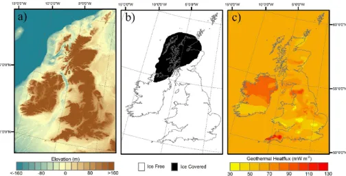
We set up the model domain to cover the entire BIIS (Fig. 2). The

easternmost domain edge runs through the North Sea, placed so that as simulated ice reaches the domain edge its normal velocity is set to zero and thus an ice divide forms. This is to represent the

effect of confluence between the BIIS and Fennoscandian Ice Sheet

in the North Sea during the last glacial cycle (Sejrup et al., 2016;

Roberts et al., 2018). This is only an approximation of the effect of

confluence, and therefore streaming features close to the eastern

margin may be susceptible to domain-edge artefacts. We use an

8 km8 km horizontal grid, with one level of re_finement at the ice

sheet margin, producing a 4 km4 km horizontal grid. The

simu-lations have 10 vertical levels. The Weertman portion of the sliding

law uses a non-linear (m¼3) exponent. We use a crevasse calving

model, which models the penetration of basal and surface crevasses (Nick et al., 2010).

To recreate isostatically adjusted bed topography, we adjust modern topography using reconstructions from a Glacio-Isostatic

Adjustment (GIA) model (Bradley et al., 2011) (Fig. 2a). GEBCO

(Becker et al., 2009) provides modern offshore bathymetry, and

SRTM (Farr et al., 2007) provides onshore topography. The Relative

Table 1

Summary of experiment set-ups. The results of sensitivity experiments (experiments with the prefix“MAX”or“MIN”) are presented inSupplementary Information S2.

Reference Start point Length (yr) SMB Geothermal Heat Flux Standard Parameter Variation

SPIN-UP N/A 20,000 Masked (Fig. 2b) 60 mWm 2 _N/A ADVANCE SPIN-UP end 10,000 0.3 m/y (>50 m a.s.l), or 0.0 m/y 60 mWm 2 _N/A RETREAT ADVANCE end 10,000 Masked onADVANCEextents 60 mWm 2 _N/A ADVANCE_

GEOTHERMAL

SPIN-UP end 10,000 0.3 m/y (>50 m a.s.l), or 0.0 m/y Variable (Fig. 3c) N/A

RETREAT_ GEOTHERMAL

ADVANCE end 10,000 Masked onADVANCE_GEOTHERMALextents Variable (Fig. 3c) N/A

MAX_FRICT ADVANCE 3,000 years 1,000 0.3 m/y (>50 m a.s.l), or 0.0 m/y 60 mWm 2 _{Weertman friction coefficient (C)}

¼6,000

MIN_FRICT ADVANCE 3,000 years 1,000 0.3 m/y (>50 m a.s.l), or 0.0 m/y 60 mWm 2 _{Weertman friction coefficient (C)}

¼1,500

MAX_TILL ADVANCE 3,000 years 1,000 0.3 m/y (>50 m a.s.l), or 0.0 m/y 60 mWm 2 _{Maximum till water depth (W}

0)¼4 m

MIN_TILL ADVANCE 3,000 years 1,000 0.3 m/y (>50 m a.s.l), or 0.0 m/y 60 mWm 2 _{Maximum till water depth (W}

0)¼1 m

MAX_COULOMB ADVANCE 3,000 years 1,000 0.3 m/y (>50 m a.s.l), or 0.0 m/y 60 mWm 2 _{Coulomb friction coef}

ficient (f)¼0.75

MIN_COULOMB ADVANCE 3,000 years 1,000 0.3 m/y (>50 m a.s.l), or 0.0 m/y 60 mWm 2 _{Coulomb friction coef}

ficient (f)¼0.25

MAX_ GEOTHERMAL ADVANCE 3,000 years 1,000 0.3 m/y (>50 m a.s.l), or 0.0 m/y 120 mWm 2 _N/A MIN_ GEOTHERMAL ADVANCE 3,000 years 1,000 0.3 m/y (>50 m a.s.l), or 0.0 m/y 30 mWm 2 _N/A

Table 2

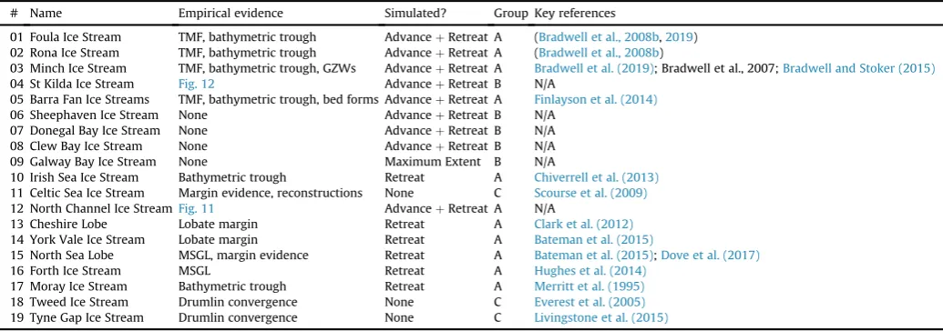
Ice streams of the BIIS, split into groups according to the availability of simulation and empirical evidence. The location of each ice stream is shown inFigs. 1 and 8.

# Name Empirical evidence Simulated? Group Key references

01 Foula Ice Stream TMF, bathymetric trough AdvanceþRetreat A (Bradwell et al., 2008b,2019) 02 Rona Ice Stream TMF, bathymetric trough AdvanceþRetreat A (Bradwell et al., 2008b)

03 Minch Ice Stream TMF, bathymetric trough, GZWs AdvanceþRetreat A Bradwell et al. (2019); Bradwell et al., 2007;Bradwell and Stoker (2015)

04 St Kilda Ice Stream Fig. 12 AdvanceþRetreat B N/A

05 Barra Fan Ice Streams TMF, bathymetric trough, bed forms AdvanceþRetreat A Finlayson et al. (2014)

06 Sheephaven Ice Stream None AdvanceþRetreat B N/A 07 Donegal Bay Ice Stream None AdvanceþRetreat B N/A 08 Clew Bay Ice Stream None AdvanceþRetreat B N/A 09 Galway Bay Ice Stream None Maximum Extent B N/A

10 Irish Sea Ice Stream Bathymetric trough Retreat A Chiverrell et al. (2013)

11 Celtic Sea Ice Stream Margin evidence, reconstructions None C Scourse et al. (2009)

12 North Channel Ice StreamFig. 11 AdvanceþRetreat A N/A

13 Cheshire Lobe Lobate margin Retreat A Clark et al. (2012)

14 York Vale Ice Stream Lobate margin Retreat A Bateman et al. (2015)

15 North Sea Lobe MSGL, margin evidence Retreat A Bateman et al. (2015);Dove et al. (2017)

16 Forth Ice Stream MSGL Retreat A Hughes et al. (2014)

17 Moray Ice Stream Bathymetric trough Retreat A Merritt et al. (1995)

18 Tweed Ice Stream Drumlin convergence None C Everest et al. (2005)

19 Tyne Gap Ice Stream Drumlin convergence None C Livingstone et al. (2015)

Sea Level (RSL) change from at 30ka BP is used to deform contemporary topography, maintaining a high-resolution ice sheet bed whilst also accounting for RSL change. RSL is constant through all experiments; the bed does not evolve after the initial RSL correction.

Calculation of the surface heatflux uses an idealised

elevation-constant surface temperature of 268 K in all experiments. In the

majority of experiments, geothermal heat_flux is uniformly set at

60 mW m 2 across the domain. In experiment GEOTHERMAL,

onshore geothermal heatflux is set to contemporary geothermal

heat_flux measurements (Busby, 2010;Farrell et al., 2014), which is

assumed an appropriate proxy for geothermal heatflux during the

last glacial cycle. Owing to the absence of sufficient measurements,

offshore geothermal heat_flux is set at 60 mW m 2.

The simulations aim to grow and shrink an ice sheet in an ide-alised cycle, rather than provide a reconstruction of the BIIS. Although a more idealised surface mass balance forcing can be used, the scheme must force a simulated ice sheet that resembles the actual evolution of the BIIS well enough so as not to impede comparisons of modelled and empirically reconstructed ice

streams, as ice stream position is in_fluenced by ice sheet geometry.

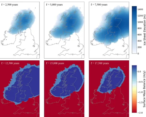
The simulations are split into three subsequent experiments with

varying surface mass balance forcing (Table 1). First, the ice sheet is

grown for 20,000 years from no ice using an ice mask (Fig. 2b). A

surface mass balance of 0.3 m/y is applied in the ice mask, and a

mass balance of 5.0 m/y applied outside the ice mask. A 2-phase

spin-up is used, with the hydrology adaptations discussed in

sec-tion2, introduced at model year 10,000 to preserve computer time

during the original build-up of the ice dome. From the end of the

SPIN-UPexperiment, an idealised climate is used to advance and

retreat the ice sheet. During theADVANCEphase, the surface mass

balance is defined as;

m¼

8 < :

0:3; h>500

0:0; h 500

2:0; h¼0:0

(5)

wheremis the annual surface mass balance (m/y), andh is the

surface elevation of ice. This forcing allows an advance that reaches a maximum extent after 10,000 years which is comparable to

empirical reconstructions (Clark et al., 2012). Every 25 years

through theADVANCEexperiment, a mask is created based on the

modelled output (Fig. 3). The mask sets values of 0.3 where the ice

sheet elevation is > 500 m, 0.0 where the ice sheet elevation is

500 m, and 2.0 where the no ice is present. Then the retreat is

forced using the masked SMB maps in reverse order, i.e. the mask produced using the 9,000 model year extent forces the 11,000 SMB,

the 8,000 year mask forces the 12,000 SMB etc. (Fig. 3). The 500 m

ELA provides a balance between too slow and too rapid retreat of the ice sheet in the retreat phase. The surface mass balance forcing is updated every 25 model years. This forcing method creates a near-symmetric pattern of advance and retreat.

3.2. Model-data comparison

We compare modelled and empirically reconstructed ice

streams, considering ice stream position, spacing,flow direction,

and evolution. To allow for consistent identi_fication of ice streams

in the simulations we define an ice stream as a region with surface

velocity exceeding 500 m/y 8 km from the margin. Qualitative comparisons between modelled and empirical ice streams were

made based on position and spacing, and_flow directions. This was

completed for topographically well-focussed ice streams since

these are the locations where the_flow direction can be empirically

reconstructed with most certainty. The empirically reconstructed

palaeoflow direction is determined as the mean orientation of the

topographic trough centreline. Together, these were used to create

a map of empirically reconstructed_flow directions for known ice

Fig. 2.Boundary conditions for the experiments, showing the full domain of the simulations. (a) Bed topography, (b) Ice mask for the ice dome produced in the spin-up simulation, and (c) Geothermal heatflux used in experiments“Geothermal”.

N. Gandy et al. / Quaternary Science Reviews 223 (2019) 105915

streams of the BIIS.

We use the tool developed byLi et al. (2007), Automated Flow

Direction Analysis (AFDA), to compare empirical and model derived

flow directions. AFDA calculates the mean residual angle and

variance of offset between modelled and empirically derived

ice-flow directions. A threshold of <10 _{mean resultant vector and}

<0.03 mean resultant variance was used to assess model-data

agreement, derived from values previously used in the literature (Napieralski et al., 2007;Ely et al., 2019).

4. Model results

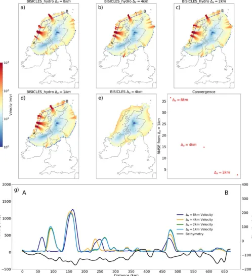
The skill of the simulations to produce ice streams of a

reason-able width, position, andflow direction is highly dependent on the

“ingredients” included in the simulations. A simulation with no

basal hydrology coupling does not simulate ice streaming (Fig. 4e).

Simulations using BISICLES_hydro achieve ice stream generation in manner that is a good match to empirical data, and demonstrates good consistency in the simulated ice stream position, spacing and

width across a range of horizontal resolutions (Fig. 4aed).

Consis-tent ice stream width means that ice catchments are also consisConsis-tent across varying horizontal resolutions, allowing margin evolution to

not vary considerably between resolutions (Fig. 4aed.). The

mini-mal resolution dependency could be explained by either the

in-clusion of membrane stresses (Hindmarsh, 2009), or topographical

constraints on both ice stream position and width. With increasing

resolution there is convergence of simulated velocity (Fig. 4f). At

4 km resolution and beyond the pattern of ice streaming is

quali-tatively and quantiquali-tatively (Table S4) similar.

4.1. ADVANCE and RETREAT

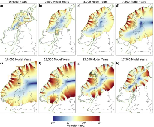
At the end of theSPIN-UPexperiment, there are four major ice

streams draining the ice sheet (Fig. 5a). As the ice sheet advances

during theADVANCEexperiment, the position of some ice streams

migrate, and the number of ice streams increases (Fig. 5aee). Some

ice streams remain spatially and temporally consistent, concurrent

with the position of ice streams marked inFig. 1, the Minch Ice

Stream [3], the Barra Fan Ice Stream [5], the Rona Ice Stream [2], and a Donegal Bay Ice Stream [7]. The Foula Ice Stream [1] is

consis-tently present from 2,500 model years onwards, but changes_flow

direction by ~45_{as the margin position changes.}

At the maximum extent of the ice sheet, at 10,000 model years (Fig. 5e), the number of ice streams around the ice sheet margin has Fig. 3.Illustration of the surface mass balance calculation for theRETREATexperiment. The top row shows simulated ice sheet elevation during theADVANCEexperiment, and the bottom row the resulting surface mass balance masks produced.

increased during theADVANCEphase. Ten ice streams have formed on the western-board of the ice sheet, which has a marine margin at the Atlantic Ocean. The areal extent here is controlled by the extent of the continental shelf, as ice cannot extend beyond the shelf break. A similar effect has been modelled on the southern margin of the Laurentide Ice Sheet, where advance into deeper

lakes initiates increased calving (Cutler et al., 2001). Ice streams are

less prominent along the southern margin, and migrate laterally

during theADVANCEphase.

During theRETREATexperiment (model years 10,000e20,000)

all the non-transitory ice streams of advance remain consistent spatially and temporally. Streaming along the southern margin Fig. 4.Variations in ice stream occurrence, position, and width. All ice surface velocity maps are at 4,000 model years into the ADVANCE experiment. a) BISICLES_hydro at 8 km horizontal resolution. b-d) BISICLES_hydro at 1, 2, and 3 levels of mesh refinement respectively. e) Without the hydrological approximation. f) RMSE of the BISICLES_hydro simulated velocities at 0, 1, and 2 levels of refinement from 3 levels of refinement. g) Ice surface velocity and bathymetry for the transect shown in panels aed.

N. Gandy et al. / Quaternary Science Reviews 223 (2019) 105915

increases, and a large ice stream forms in the Irish Sea (Fig. 5f). Smaller ice streams form onshore, concurrent with the Vale of Cheshire and York, although these stop streaming by 15,000 model

years (Fig. 5g and h). At 12,500 model years, two large ice streams

drain the ice sheet on the eastern domain edge in the North Sea. These large features are an artefact of the ice sheet being separated

from the domain edge following con_fluence during theADVANCE

experiments, and therefore are not comparable with the empirical record. Once the ice sheet is separated from the eastern domain edge (~15,000 model years), ice streams in the North Sea area have a comparable size and spacing to other ice streams simulated around the margin.

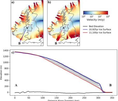
During the ice sheet advance, steeper margin and shallow

interior surface slopes occur along the southern margin (Fig. 6), as

is expected on an advancing margin. In the retreat phase the SMB imposes melting at the southern margin of the ice sheet. This lowering steepens the ice surface at the ice stream onset zone, accelerating ice streaming and resulting in a shallower surface

pro_file downstream of the onset zone. This means that during the

advance phase there is only extensive streaming along the northern margin, whilst streaming also occurs along the southern margin

during the retreat phase (Fig. 6). The feedback between SMB and ice

stream behaviour has been demonstrated numerically (Robel and

Tziperman, 2016), and this effect has been shown to promote rapid deglaciation. Experiments of the evolution of the BIIS with a realistic climate forcing also produce ice streams with high

tem-poral variability (Hubbard et al., 2009).

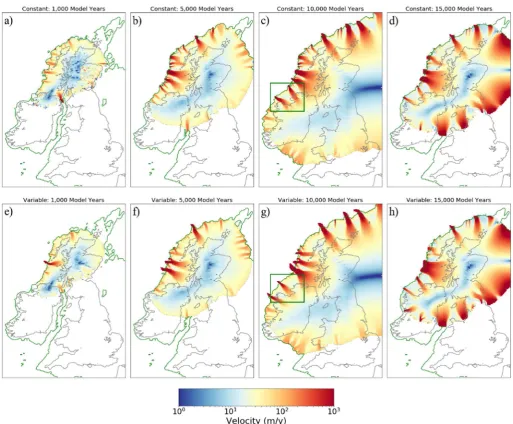
4.2. Variable geothermal heatflux

Introducing a spatially variable geothermal heat_flux produces

limited changes to the pattern of ice streaming simulated for most of the ice sheet. The width and spacing of the ice streams is almost

identical (Fig. 7). The dominant ice streams identi_fied from the

ADVANCEandRETREATexperiments (i.e. coincident with the Minch Ice Stream, and the Barra Fan Ice Streams) remain constant in the

variable geothermal heat_flux experiments. The region of highest

geothermal heat_flux in the domain, in South-west England, is not

Fig. 5.Ice velocity at 2,500 model year intervals during theADVANCE(aee) andRETREAT(feh) experiments. Orange boxes highlight ice streams with significant empirical evidence

(Fig. 9). Green boxes highlight ice streams with empirical evidence presented in this research (Figs. 11 and 12). The green contour shows the 0 m bed elevation, and the ice sheet grounding line. An animation of the experiment is contained in thesupplementary information (S3).

covered by ice, both in these simulations and according to empirical

reconstructions (Clark et al., 2012), so has no impact on the ice

stream dynamics simulated. Other comparative “hot spots” also

produce a minimal effect, despite being ice covered. The higher

geothermal heat _flux over the North of Ireland does not cause

significant change in the margin position as the ice sheet advances

over Ireland (Fig. 7b,f).

The primary change in the ice stream con_figuration is on the

west coast of Ireland, where the geothermal heat_flux is

compara-tively high (Fig. 2c). In the spatially constant geothermal heatflux

experiment an ice stream is simulated coincident with Donegal Bay (Fig. 1[7]), with a second ice stream to the north in the Sheephaven

ice stream region (location indicated inFig. 1[6]). In the spatially

variable geothermal heat flux experiment, an ice stream is still

simulated in Donegal Bay, but to the south in Clew Bay rather than

the north (Fig. 1[8]). In this region of the ice sheet, there are no

significant bathymetric troughs, suggesting that variable

geothermal heat _flux becomes a comparatively more signi_ficant

control on ice stream form and location in western Ireland than the

rest of the BIIS. This demonstrates that geothermal heatflux can be

an important control on ice stream location, but only in regions

where other more signi_ficant controls, like topographic troughs, are

not present. Including a spatially variable geothermal heatflux is

not a necessary ingredient for modelling the majority of ice streams of the BIIS when using the physics in BISICLES_hydro, but is more

influential on the western Irish coast.

5. Model-data comparison

We compare simulated and empirically-based ice streams using both qualitative comparisons of position and spacing and a quan-titative tool. Ice streams of the BIIS are split into three categories; ice streams that are simulated by the model and have empirical evidence (group A), ice streams that are simulated by the model but have no empirical evidence yet published (group B), ice streams that are not simulated but have been reconstructed empirically (group C). The majority of ice streams simulated here (11/17) are

supported by empirical evidence (Table 2).

5.1. Group A

Group A are the eleven BIIS ice streams simulated here and

supported by the empirical record (Table 2). Four of the most

consistent ice streams in the simulations coincide with the Fig. 6.Transect of the ice surface at a period before and after the onset of significant ice streaming in the Celtic Sea (10,925 and 11,100 model years respectively). Grey curves show the ice surface at 25 year intervals between the two snapshots.

N. Gandy et al. / Quaternary Science Reviews 223 (2019) 105915

locations of the four ice streams with the strongest empirical evi-dence. Each of the ice streams (the Barra Fan Ice Streams, the Minch Ice Stream, the Rona Ice Stream, and the Foula Ice Stream) are

associated with a clear bathymetric trough (Fig. 9), and terminate at

major Trough Mouth Fans (Bradwell et al., 2008b). These are thick

accumulations of sediment fed across an ice stream marine margin (Vorren and Laberg, 1997). The bathymetric troughs and associated Trough Mouth Fans are strong empirical evidence of sustained ice

streaming, which the model here shows signi_ficant skill in

simulating.

A number of ice streams in Group A form in bathymetric troughs, and therefore locational (or colocation) between the reconstructed and simulated ice streams was likely. However, some of the Group A ice streams form in relatively minor bathymetric troughs, like the North Sea Lobe, the Forth Ice Stream, and the Moray Ice Stream. In these examples, the simulations show

sig-ni_ficant skill in simulating empirically reconstructed ice streams

with subtle bathymetric confinement. Although bathymetry does

not directly control the position of these ice streams, neighbouring

trough controlled ice streams can in_fluence their position. This

means that the skill of the model in simulating ice streams in

sig-nificant bathymetric troughs allows the model to show skill in

simulating ice streams away from bathymetric troughs.

The empirically well-constrained ice streams in bathymetric troughs allow a quantitative comparison between simulated ice streams and empirically reconstructed ice stream paths using AFDA (Li et al., 2007;Napieralski et al., 2007;Ely et al., 2019). The Auto-mated Flow Direction Analysis (AFDA) tool calculates the mean residual vector and variance between simulated and reconstructed ice _flow. Fig. 10 shows the resulting mean residual vector and

variance of theflow direction for the duration of each ice stream's

simulation. The Rona Ice Stream (Fig. 10b) is the strongest match

between simulated and empirical evidence, with an average mean

residual vector of 5_{, and only brief excursions above the}

data-model match criteria. The Minch and the Barra Fan Ice Streams

also perform reasonably well during periods of theADVANCEand

RETREATexperiments.

The Foula ice stream is the shortest-lived ice stream, streaming

from 8,500 to 15,000 model years (Fig. 5e and f), and matches

empirical_flow directions at the start and end of the ice stream's

Fig. 7.Ice velocity at 5,000 year intervals for theADVANCEandRETREATexperiments with a spatially uniform geothermal heatflux (aed), and a spatially varied geothermal heatflux

(eeh). The green box in panel c and g highlight the key region of difference between the experiments.

existence, but there is no model-data match during the majority of

the ice stream's occupancy. There is significant flow direction

change of the Foula ice stream during the simulation, as the shape

of the margin changes during con_fluence with the eastern domain

edge.

The results from AFDA con_firm the qualitative conclusion that

for many ice streams there is often a strong match between model and empirical data. The empirically best-constrained ice streams of

the ice sheet form in significant bathymetric troughs (Fig. 9), which

the model demonstrates signi_ficant skill in simulating. Whilst there

may be a weaker model match for ice streams that are less bathy-metrically controlled, like the North Sea and western Irish margin,

the empirical reconstruction of _flow direction is also less well

constrained in these regions. The AFDA scores are sensitive to variations in the empirical reconstruction, so poorly constrained ice streams are not suitable for meaningful comparison.

A number of simulated ice streams are more prominent during the retreat phase than the advance phase. These ice streams include the Moray Firth Ice Stream, the North Sea Lobe, and the Irish Sea Ice Stream. The retreat forcing increases the propensity of the ice sheet

to stream along the southern margin (Robel and Tziperman, 2016).

The simulated ice streams of the retreat phase generally form in positions with strong empirical evidence, like the North Sea Lobe (Dove et al., 2017). Ice streams that are simulated only during the

retreat of the ice sheet form in less significant bathymetric troughs

that the Minch, Barra Fan, Foula, and Rona Ice Streams. It seems, therefore, that these have a lower propensity to stream, until triggered by the ice sheet retreat.

5.2. Group B

Simulated ice streams without published empirical evidence form the second largest group of ice streams of the BIIS; group B (Table 2). Empirical evidence for ice streaming is inconsistently preserved by subsequent erosion and deposition. Because of this, the empirical record is, and will always be, incomplete. Given the

apparent skill of the model (Group A), that ice streams may be simulated which are currently unmapped, is not a basis for dis-counting the model results.

The presence of simulated ice streams with no published empirical evidence stimulated us to conduct a re-examination of the empirical record in these areas. This is most prominent for the Irish west coast, where a number of ice streams are simulated, but without empirical evidence for streaming reported. Here, high rates of sedimentation during the Holocene may be obscuring

bathy-metric troughs and subglacial lineations. In the future, re_flection

seismic data may reveal these features.

In other areas, improved bathymetric data coverage allows new mapping to reveal evidence of ice streaming in regions simulated

here. A North Channel Ice Stream,_flowing in the Irish Sea west of

the Isle of Man, is simulated in the advance and retreat of the ice

sheet (Fig. 5). Recent bathymetric multibeam data, from the UK

Hydrographic Of_fice with point data gridded into an 8 m horizontal

grid, allows major subglacial lineations in this region to be mapped (Fig. 11). Two hill-shades were created for the gridded bathymetric

data, illuminating from 045 _{to 315 to avoid azimuth biasing}

(Smith and Clark, 2005). Hill-shaded bathymetry is overlain with translucent bathymetry to aid with geomorphological feature mapping. The mapped subglacial lineations are elongate (typically

2e6 km long and 100s of m wide), indicative of high ice velocities

(Clark, 1993;Stokes and Clark, 1999;Spagnolo et al., 2014;Ely et al.,

2016). This example demonstrates how model results can motivate

and steer empirical work, here leading to the identification of a

North Channel palaeo-ice stream that has not been previously documented.

A St Kilda ice stream (_flowing just south of the Scottish

archi-pelago St Kilda) is also consistently simulated throughout the glacial cycle. Here, the bathymetric data does not provide evidence for subglacial lineations, but there is some circumstantial evidence

for ice streaming (Fig. 12). A small bathymetric trough is evident,

encouraging ice_flow between South Uist and Barra. The region is

predominantly exposed bedrock, potentially caused by the Fig. 8.Ice velocity at 10,000, 12,500, and 15,000 model years. Locations of key ice streams empirically reconstructed in the literature are highlighted with black arrows, with ice streams numbered as inFig. 1andTable 2. The wide ice streams in the North Sea are caused by a domain-edge effect.

N. Gandy et al. / Quaternary Science Reviews 223 (2019) 105915

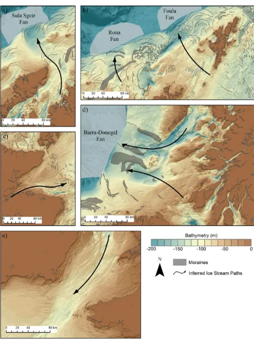
Fig. 9.Bathymetry and geomorphological landforms offive empirically well constrained ice streams, a) The Minch Ice Stream, b) The Foula and Rona Ice Streams, c) The Moray Firth Ice Stream, d) The Barra Fan Ice Streams, and e) the Irish Sea Ice Stream.

extensive ice stream erosion (e.g.Bradwell et al., 2008a;Newton et al., 2018). Whilst the evidence for the North Channel Ice Stream is direct, the empirical evidence for a St Kilda Ice Stream remains circumstantial. However, the model results could encourage more targeted empirical data collection to investigate the evidence for a palaeo-ice stream.

Overall, whilst the majority of ice streams simulated have strong evidence in the empirical record, there are a handful of ice streams simulated with no empirical evidence. This offers an opportunity

for targeted empirical data collection and analysis tofind evidence

for or against ice streams simulated in these experiments, which is

supported by increasing quality of bathymetric products (Becker

et al., 2009; Calewaert et al., 2016), and greater collection of

shallow reflection seismic data (O'Brien et al., 2016;Stewart, 2016).

5.3. Group C

A small number of BIIS ice streams have empirical evidence but Fig. 10.Mean residual vector and mean residual variance between modelled and empirically reconstructedflow for four simulated ice streams. Dashed lines show the threshold mean residual vector and mean residual variance used to identify model-data agreement. The yellow highlight shows times of model-data agreement.

N. Gandy et al. / Quaternary Science Reviews 223 (2019) 105915

Fig. 11.Subglacial landform mapping of the North Channel Ice Stream. a) Seafloor bathymetry, and b) Resulting map of elongate subglacial bedforms.

Fig. 12.Bathymetry of the path of the simulated St Kilda ice stream. Bathymetry data source: UKHO and GEBCO.

are not simulated here (Group C). This includes the Tweed Ice

Stream (Fig. 1[18]), evidenced by extensive mapping of streamlined

subglacial bedforms (Everest et al., 2005). The_flow of the Tweed Ice

Stream is dependent on margin positions in a complex region of the

ice sheet (Livingstone et al., 2015). The simulations here are not

intended to be a margin reconstruction of the BIIS, and do not include the complex margin history expected in this region.

The Celtic Sea Ice Stream is the ice stream of the BIIS with the greatest width that is not consistently present in the simulations. The southern margin of the simulated ice sheet in the Celtic Sea

never reaches as far south as empirical reconstructions (Scourse

et al., 2009). The limited model extent compared to empirical data in this region may be due to a lack of persistent ice streaming during the advance phase, the lack of a simulated large surge event,

or because the idealised SMB forcing in this case is suf_ficiently

different than reality in this sector. Whilst the empirical evidence is

able to constrain the extent of the Celtic Sea Ice Stream (Scourse

et al., 2009; Praeg et al., 2015), the flow geometry is difficult to reconstruct owing to a lack of subglacial bedforms. The differences in the empirical evidence between the Celtic Sea Ice Stream and other ice streams of the BIIS, along with the low model skill compared to high skill for other ice streams, suggests that the Celtic Sea Ice Stream was mechanistically different to the other ice streams of the BIIS.

6. Discussion

6.1. Required ingredients for modelling ice streams

Here we discuss which model ingredients are crucial to suc-cessfully model ice streams, which are desirable, and which can be deemed as not important. The most important model ingredient in these experiments is the representation of idealised subglacial hydrology, in these experiments as a till-water layer coupled with

the Coulomb portion of the sliding law, as without this the ice sheet

model does not spontaneously generate ice streams (Fig. 4e). An

adequate horizontal resolution is also an important model ingre-dient, the Minch Ice Stream modelled down to 4-1 km resolution (Fig. 4d) achieves an improved AFDA score than when it is

simu-lated at 8 km resolution (Table S4). However, lower-order models

experience more significant resolution dependency (Hindmarsh,

2009), and if an experiment was also considering grounding line

dynamics using a model of suf_ficient physical complexity, like

BISICLES, could also be considered a crucial model ingredient. Depending on the context of the experiments, additional model

ingredients are required. The representation of SMB has an in_fl

u-ence on ice stream behaviour, evident by the increased streaming

along the BIIS southern margin when SMB became negative (Fig. 6),

and previous experiments (Robel and Tziperman, 2016). An

accu-rate SMB also has a number of secondary effects. For example, ice streams of central northern England were likely not simulated here because they are dependent on complex margin and ice dome changes that cannot be simulated with an idealised SMB scheme. A

spatially variable geothermal heatflux was also determined to be

non-crucial for the BIIS but might be important for simulating ice streams of other ice sheets, like the Northwest Greenland Ice

Stream (Rysgaard et al., 2018). Previous simulations of ice streams

of the BIIS also used a spatially uniform geothermal heat flux

(Hubbard et al., 2009).

Finally, some model ingredients were either ignored or highly idealised in this study and are not important in this experimental context. For example, a good match to empirical data was achieved

despite a spatially uniform Weertman coef_ficient, Coulomb friction

angle, maximum till-water depth, and till-water drain rate. Varying

these parameters does change the pattern of ice streaming (Fig. S2),

but representing these factors as spatially variable is not a neces-sary model ingredient in this case. However, a more realistic rep-resentation of the subglacial environment, including factors such as Fig. 13.a) Ice Velocity att¼4,000 years. b) Till water thickness att¼4,000 years.

N. Gandy et al. / Quaternary Science Reviews 223 (2019) 105915

variable bed geology, and/or improved process understanding may

prove to be a more influential model ingredient for other ice sheets,

and could help improve the simulation of the Celtic Sea Ice Stream. The horizontal transport of meltwater is a process that remains unrepresented in the model. The supraglacial, englacial, and sub-glacial transport has been observed to redistribute water on short

timescales (Andrews et al., 2014), and has been identi_fied as a key

control on ice sheet velocity (Zwally et al., 2002; Hewitt, 2013).

Meltwater transport also evolves annually (Chandler et al., 2013),

and is expected to be a mechanism to cause ice stream evolution.

Although the experiments here achieve a closefit to empirical data

without a representation of horizontal meltwater transport, future model development should include this mechanism and test for its

influence in a variety of ice sheet contexts.

6.2. Ice stream controls

Winsborrow et al. (2010)reviewed the literature on palaeo and contemporary ice streams, and compiled seven factors that control ice stream location. They are, in the order of importance that

Winsborrow et al. (2010)proposes, topographic troughs, marine margins, soft beds, abundant meltwater, smooth beds, high

geothermal heat_flux, and topographic steps. Whilst ice streams

will spontaneously form due to thermo-mechanical coupling of ice

flow (Payne and Dongelmans, 1997), these seven factors controls the relative position of ice streams. Of the seven factors, only soft beds are not represented in these simulations as bed friction

co-efficient is idealised to be uniform across the domain.

For the BIIS, the in_fluence of topographic troughs and steps are

considered together, as the features co-exist at the ice sheet bed.

Supporting the Winsborrow et al. (2010) hierarchy of controls,

these simulations suggest that bed topography is the primary control of ice stream location for the BIIS. The primary large, and spatially and temporally consistent ice streams in the simulations, are all located in bathymetric troughs; the Minch Ice Stream, the Barra Fan Ice Streams, the Rona Ice Stream, and the Foula Ice Stream (Fig. 9). However, not all simulated ice streams form in well-defined topographic troughs, like the North Sea Lobe, Forth Ice Stream, and the ice streams of the Irish west coast. Ice streams without

well-defined topographic control are more likely to be sensitive to

weaker controls on ice stream location, demonstrated by the change in ice stream location in Northwest Ireland when

consid-ering a varying geothermal heatflux (Fig. 7). Ice streams outside a

topographic trough also exhibit greater resolution dependency (Fig. 4g). An idealised experiment of a square ice sheet on a_flat bed (Fig. S1) also shows greater resolution dependency than on a real

bed (Fig. 4), suggesting that these ice streams may also be more

sensitive to resolution.

The position of topographically controlled ice streams has an indirect control on ice streams with weaker topographic control. It

has been shown here (Fig. S1), and in previous research (Payne and

Dongelmans, 1997; Hindmarsh, 2009) that even on a _flat bed regularly spaced ice streams will form around the margin of an ice sheet. Therefore, whilst topographic troughs will determine the location of some of the ice streams of the BIIS, other ice streams

would be expected to form between these ice streams even onflat

beds. Ice sheet models onflat beds predict regular spacing of ice

streams; but on a real bed with topographic variation, some ice streams would be anchored in topographic troughs and the

pre-dominant spacing control then fixes the position of other

non-topographic ice streams.

The simulations also support the expected strong in_fluence of

marine margins, with the most spatially and temporally consistent ice streams occurring along the western board of the ice sheet, with a marine margin in the Atlantic Ocean. Many simulated ice streams

with a marine margin are also in bathymetric troughs, although the ice streams of the western Ireland coast have a marine margin without large troughs. Calving at the margin of the ice sheet lowers

the surface pro_file, allowing the capture of more ice from the

catchment, and thus increased ice streaming. Ice streams that advance and retreat onshore, for example through central and

southern England (Fig. 5d and e), do not stream constantly, unlike

the majority of ice streams with a marine margin. Therefore, there is evidence from these simulations that a marine margin is a strong control of behaviour of BIIS ice streams, but not necessarily ice stream location.

The saturation of the till-water layer is a control on the water pressure, which is in turn a variable in the Coulomb portion of the

sliding law. The saturation of the till-water layer is influenced by

the geothermal heatflux, maximum till-water layer thickness, and

the till-water drain factor. Whilst there is a strong relation between the location of modelled ice streams and regions of a saturated

till-water layer (Fig. 13), the till-water layer saturation is not the sole

control on ice stream position. On the southern and eastern margin there are a number of regions of saturation, whilst ice streaming does not occur. However, no ice streams are apparent in regions with low till-water layer saturation. The increased velocity of an ice stream increases frictional heating, and therefore increases the saturation of the till water layer. The relationship between the saturation of the till-water layer and ice velocity means evidence of

cold-based ice (Bierman et al., 2015;MacGregor et al., 2016) can be

a strong constraint on model results.

The relatively limited influence of the geothermal heatflux is

highlighted by the experiments ADVANCE_GEOTHERMAL and

RETREAT_GEOTHERMAL, suggesting that the spatial distribution of

geothermal heatflux is only a weak control on the formation and

location of ice streams. The most signi_ficant difference to ice

streaming made by a spatially variable geothermal heat_flux is in

western Ireland, where the influence of bathymetric troughs is

weak. The relatively small in_fluence of geothermal heat _flux has

been supported by Winsborrow et al. (2010). However, it is

important to note that there is only a limited range of geothermal

heatflux values across the domain. Geothermal heatflux could be

an important control of ice stream formation and location in do-mains with weaker other controls on ice stream location and a

wider range of geothermal heat flux values. For example, it has

been suggested that the location and unusual geometry of the

Northeast Greenland Ice Stream may be influenced by a geothermal

heatflux hot spot at the ice sheet bed (Rysgaard et al., 2018).

6.3. Model evaluation

The comparison between the simulated and empirically recon-structed ice streams can be used to evaluate the skill of the ice sheet model at producing ice streams in reasonable locations. The qual-itative and quantqual-itative similarities between the simulated ice streams and the ice streams recorded in the empirical data suggests

that the model has significant skill. The simulations consistently

produce ice streams in areas of strong empirical evidence. There-fore it would be reasonable to apply this to other palaeo ice sheets where the empirical record is less complete. If the model can consistently simulate expected ice stream and ice sheet evolution over millennia for a diverse range of palaeo ice sheets, the model

would be expected to have suf_ficient skill to project medium- and

long-term evolution of the Greenland and Antarctic Ice Sheets. However, some mechanisms not represented in the model,

which could be in_fluential to ice stream formation and location,

including water drainage from the ice surface to the bed (Das et al.,

2008; Krawczynski et al., 2009), and ice stream freeze on and

shutdown (Christoffersen and Tulaczyk, 2003). These simulations