Statistical Modelling of Pitting Corrosion: Extrapolation of the Maximum Pit Depth-Growth

Int. J. Electrochem. Sci., 9 (2014) 4129 - 4143

International Journal of

ELECTROCHEMICAL

SCIENCE

www.electrochemsci.org

Statistical Modelling of Pitting Corrosion: Extrapolation of the

Maximum Pit Depth-Growth

J.C. Velázquez1,*

, J.A.M. Van Der Weide2, Enrique Hernández3, Héctor Herrera Hernández.4,**

1 _{Departamento de Ingeniería Química Industrial, IPN-ESIQIE, UPALM Edif. 7, 1}er

Piso, Zacatenco, 07738, México D.F., México.

2

Faculty Electrical Engineering, Mathematics and Computer Science, Delft University of Technology, Delft, The Netherlands.

3

Departamento de Bioingeniería, Instituto Politécnico Nacional-UPIBI, Av. Acueducto s/n, Barrio la laguna Ticomán, 07340, México D.F., México.

4

Universidad Autónoma del Estado de México, Ing. Industrial, Blvd. Universitario s/n, Predio San Javier Atizapán de Zaragoza, Edo. de México,54500, México.

*

E-mail: [email protected]*, [email protected]**

Received: 5 February 2014 / Accepted: 22 April 2014 / Published: 19 May 2014

Pitting corrosion is one of the main threats in the pressure vessels integrity and also causes the failure of buried pipelines steels that transport sour gas, crude oil or condensate hydrocarbon, for this reason, a reliability assessment of pressurized vessels and buried pipelines based on probabilistic mathematical modelling to estimate the remaining life-time due to pitting corrosion damage is extensively employed. Herein, a methodology for probabilistic mathematical modelling of the pits initiation process and its depth growth process is developed; both uncertain processes are well represented by stochastic models. In this methodology two stochastic models are applied; Poisson process is used to model pit initiation and Gamma process to model the pit depth-growth. Such methods are validated using data produced by computer modeling procedures. On the other hand, in the oil industry it is common not to inspect the entire vessels surface; instead of this only a small part of the surface is under inspection. According to this, the use of Block Maxima (BM) and Peak-Over-Threshold (POT) models “EXTREME VALUE STATISTICS” to characterize the probability distribution of maximum pit depths is also approached. The results indicate that POT model can evaluate efficiently the maximum pitting corrosion depths.

Keywords: Pitting corrosion, Stochastic models, Pressure vessels, Steel pipelines.

1. INTRODUCTION

the case of the almost 4 million kilometer of metallic pipelines crossing the U.S. [2], the cost could exceed the 8.6 billion dollars per year [3]. Some studies around the world have found that one of the main threats of the pipelines integrity is the pitting corrosion [4-7]. This phenomenon has great importance for the maintenance of metallic structures. The documented stochastic nature [8] and the lack of an electrochemical technique capable to estimate the pit depths make that the pitting corrosion would be usually modeled using probabilistic and statistics techniques.

In order to model the pitting corrosion it is necessary to pay attention in the two main steps of this degradation process: the initiation and the growing. The pit initiation time can be described using a Poisson distribution [9]. Initially, the pitting growth was modeled using deterministic models. The most famous deterministic approach to represent the pitting growth is a power law proposed by Romanoff [10] the last century:

( ) q

y t kt (1)

Where: y t( ) is the pit depth, t is time, k and q are regression parameters.

More recently, some studies [11-12] have showed that it is possible to relate the k and q

parameters with the characteristic of the environment. However, there are other factors such as the alloy composition, microstructure, non-homogeneity of the surrounding media, temperature, that make difficult the accuracy of a deterministic approach. For this reason, it is more useful to develop models that can represent the variability of the response. Therefore, in recent times, some authors have been created stochastic models that include the power law mentioned above taking into account soil characteristics [13-15].

The main goal to study the pitting corrosion like a stochastic phenomenon is to assess the risk of perforation of in-service components. By thinking in this way, it is important to focus on the analysis of maximum pit depths because the deepest pits are the first pits that cause leaks. To study the deepest pits is frequently to make use of the extreme value theory [8, 12-14].

In the oil and gas industry there are some structures that are not possible to inspect like unpiggable pipelines or some parts of the pressure vessels. In those cases, it is helpful to employ the sampling inspection. The samples are used to estimate the deepest pit in a pressure vessel using the concept of return period.

The Gumbel distribution is usually used to estimate the maximum pit depth via Block Maxima (BM) [16, 17]. Nevertheless, Caleyo et al.[15] showed that the application of the Generalized Extreme Value Distribution (GEVD) can be more appropriate than any other bi-parametric distribution (e.g. Gumbel, Weibull or Fréchet). The expression that represents GEVD is described by Equation (2) [18]. This equation is defined on









    , the scale parameter 0 and the location parameter     .

1/

( ) exp 1 M

M

y G y

 

 _{   } 

 

 _  _{   }



 

 

 

 

Caleyo et al.[15] also fitted the maximum pit depth to GEVD and they noticed that the shape parameter progresses in time. But, one can ask the next question: Can be noticed the evolution of the shape parameter when it is only inspected a small part of the structure? This research helps to answer this question.

This paper describe the pit initiation time like a Non-Homogeneous Poisson Process (NHPP) [19].The pitting growing is modeled using the Gamma process [20,21]. Once, the pit depth is obtained, it is possible to study the maximum pit depths using both the Block Maxima (BM) and the Peak-Over-Threshold (POT) methods

2. PIT INITIATION MODELLING

The pits usually initiate at random times and they grow according to the natural characteristics of the material and the environment. That is why we model the initiation time and the total number of pits up to certain time assuming that the number of pits in time follows a NHPP.

It is feasible to suppose that the pit initiation time also arises according to a NHPP with intensity function m t( ), where  is defined as the mean pit density per area unit and m t( ) can be an arbitrary function. In accordance with the last supposition the expected number of pits up to time t can be described using the Expression (3) [20].

0

( ( ) ) ( ) ( )

t

s

E N t m s M t



  

_

The meaning of the Equation (3) is that given both the mean pit density and the intensity function the number of pits follows a Poisson distribution. It is possible to represent the increment of the actual number of pits N t( )i N t( )i N t(i1) where t0   t1 t2 ...are different times. This

supposition implies that N t( )1  N t( )2 ...are independent and each one can be described according

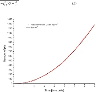
to the Equation (4). Where x N t( )i . The Figure 1 shows an example of the evolution of the number

of pits.





1

( ( ) ( ))

( ) exp ( ( ) ( )

!

x

i i

i i

m t m t

P x m t m t

x



 

   (4)

s (t_i2t_i2_1)Ut_i2_1 (5)

0 1 2 3 4 5 6 7 8

0 100 200 300 400 500 600 700 800 900 1000 1100 1200 1300 1400

Poisson Process (=20, m(t)=t2₎

f(t)=20t2

N

u

mb

e

r

o

f p

its

Time [time units]

Figure 1. Number of pits evolution.

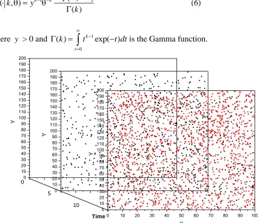
Just for the sake of illustration, it is showed the evolution in time of the simulated pits in Figure 2. This figure exemplifies how the number of pits increases in time. The black points represent the pits that start to grow between time zero and five units, while the red points represent the pits that start to grow between time five and ten units. The pits location is also simulated using the Uniform distribution.

3. PITTING GROWTH MODELLING

It is well accepted that the pitting growth can be modeled by statistics methods [11-15, 21-22]. One of the methods that can be used is the Gamma Process [20-21]. The Gamma Process is a continuous-time stochastic process with independent gamma increments. The shape parameter (k) controls the rate of the jump and the inverse of the scale parameter () controls the jump sizes. The Gamma Process with shape parameter k > 0 and scale parameter  > 0 is a stochastic process





2. for all ti ti10 and

3. y t( ) has independent increments.





1 exp /

( , )

( )

k k y

Ga k y

k

   

   

 (6)

Where y > 0 and 1 0

( ) k exp( )

t

k t t dt

 



 



0 10 20 30 40 50 60 70 80 90 100 110 120 130 140 150 160 170 180 190 200 Y 0 10 20 30 40 50 60 70 80 90 100 110 120 130 140 150 160 170 180 190 200 Y

0 10 20 30 40 50 60 70 80 90 100

0 10 20 30 40 50 60 70 80 90 100 110 120 130 140 150 160 170 180 190 200 Y X 0 5 10 Time

Figure 2. Evolution of the pits location with =20 units. The black points represent the pits that appear

between time zero and five units, while the red points represent the pits that appear between time five and ten units.

By the considerably divisibility of the Gamma distribution, the Gamma distribution is a Lévy process. A Lévy process can be written as the sum of Brownian motions. It means the sum of random increments.

Using this way of modelling, it is possible to represent the linear behavior of the pitting growth. Although, the linear pitting growth modelling is commonly used in the industry in order to calculate the estimation of the remaining life-time of the pressure vessels, in the strict point of view, the pitting corrosion growth has a non-linear behavior [10-12]. Considering this non-linear behavior, the overestimation can be reduced. For this reason, in this research it is combined the deterioration process considering a non-linear behavior and the Gamma process. Hence, we modify the second property of

the Gamma process mentioned above, for this one: where

q is the parameter that represents the nonlinearity growth of the pitting corrosion. Usually, the

qparameter is less than or equal to unity. Velazquez et al.[12] proposed to determine the q parameter value taking into account the soil characteristics. In this way, it is possible to relate the corrosion theory and the stochastic characteristic of the pitting growth.

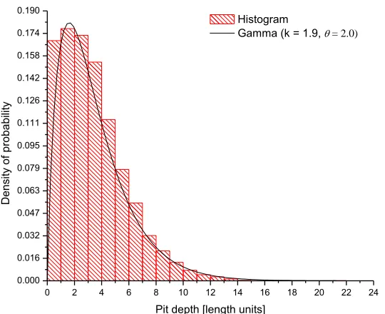
confidence bands, all the paths must be inside of these ones. Just for the sake of illustration, the Figure 4 shows the pit depth histogram at time 25 units with =20 units and q=0.6. The line correspond to the gamma pdf fitted, according to the gamma process theory, the result of the sum of the all increments must be also a gamma distribution.

0 2 4 6 8 10 12 14 16 18 20

0 1 2 3 4 5 6 7 8 9 10 11 12

Mean

Confidence Bands

T

ime

[t

ime

u

n

its]

Depth [length units]

k=1  q=0.6

Figure 3. Random paths. The solid line shows the mean and the dotted lines show the confidence

bands at 95%.

0 2 4 6 8 10 12 14 16 18 20 22 24

0.000 0.016 0.032 0.047 0.063 0.079 0.095 0.111 0.126 0.142 0.158 0.174 0.190

Histogram

Gamma (k = 1.9,= 2.0)

D

e

n

si

ty

o

f p

ro

b

a

b

ili

ty

Pit depth [length units]

4. EXTREME VALUE ANALYSIS

In the extreme value theory, there are two approaches to analyzed the maximum values. The first is named Block Maxima (BM); these models consider the largest observations obtained from blocks. In our research each block is a small area of the total. Another approach is named Peak-Over-Threshold (POT); these models focus on the observations which exceed certain threshold.

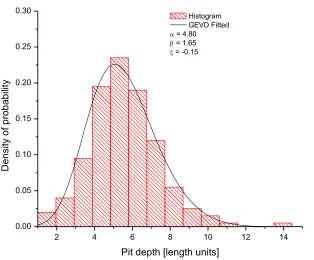
In this research, a rectangle is used to represent a steel plate. This rectangle has an area of 100 x 200 units. We divided this rectangle in small blocks with area of 10 x 10 units. Using this method it is reasonable to study the distribution of the deepest pits. The Figure 5 is an example of the maximum pit depth simulated at time 10 with =20 and q=0.7.

2 4 6 8 10 12 14

0.00 0.05 0.10 0.15 0.20 0.25 0.30

Histogram GEVD Fitted

 = 4.80

 = 1.65

 = -0.15

D

e

n

si

ty

o

f p

ro

b

a

b

ili

ty

Pit depth [length units]

Figure 5. Histogram of the maximum pit depth using BM with =20 and q=0.7 at time 10. The black

line represents the GEVD fitted.

The histogram is fitted to GEVD, using the Kolmogorov-Smirnov test [24]. The parameters value obtained during the fitting are presented in this figure. It is possible to observe that the shape parameter is a “little bit” lower than zero.

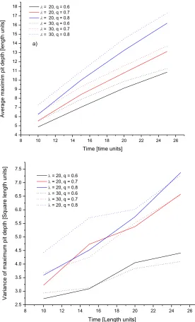
Non-parametric estimates of the median and variance of the simulated values were obtained from the simulations done with the conditions mentioned above. From Figures 6a and 6b it is possible to observe that the median and the variance tend to increase in proportion to time. Similar results were obtained by Caleyo et al.[15] in a Monte Carlo study about the maximum pit depth evolution, concluding that the variance increase in time because of the pits stochastic nature. In longer time the variance increases because the older pits continue growing and new pits keep appearing.

8 10 12 14 16 18 20 22 24 26

4 5 6 7 8 9 10 11 12 13 14 15 16 17 18

Ave

ra

g

e

ma

xi

mi

m

p

it

d

e

p

th

[l

e

n

g

th

u

n

its]

Time [time units]

 = 20, q = 0.6  = 20, q = 0.7  = 20, q = 0.8  = 30, q = 0.6  = 30, q = 0.7  = 30, q = 0.8

a)

8 10 12 14 16 18 20 22 24 26

2.5 3.0 3.5 4.0 4.5 5.0 5.5 6.0 6.5 7.0 7.5

Va

ri

a

n

ce

o

f

ma

xi

mu

m

p

it

d

e

p

th

[

Sq

u

a

re

le

n

g

th

u

n

its]

Time [Length units]

 = 20, q = 0.6

 = 20, q = 0.7

 = 20, q = 0.8

 = 30, q = 0.6

 = 30, q = 0.7

 = 20, q = 0.8

Figure 6. Time evolution of the non-parametric estimates; (a) mean and (b) variance of the simulated

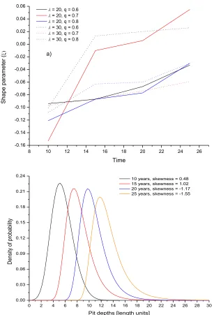
The shape parameter also increases in proportion to time (see Figure 7a). We can observe in this figure that the shape parameter goes from the negative to positive values. It means that Weibull distribution is the best option for short-term exposures. For long-term exposure Gumbel or Frechet can be a better option. Caleyo et. al.[15] also observe this behavior. They conclude that the increment in the shape parameter can be related with the fact that, for longer times the deepest pits continue growing. This evolution provokes that the maximum pit depth distribution skew toward deeper pits and the tail turn out to be larger. In the Figure 7b one can notice the effect of the shape parameter changes in the “bell curve”. In fact, the skewness values for each distribution change from positive to negative. This effect can affect considerably the probability of leakage.

8 10 12 14 16 18 20 22 24 26

-0.16 -0.14 -0.12 -0.10 -0.08 -0.06 -0.04 -0.02 0.00 0.02 0.04 0.06

Sh

a

p

e

p

a

ra

me

te

r

(



Time

 = 20, q = 0.6

 = 20, q = 0.7

 = 20, q = 0.8

 = 30, q = 0.6

 = 30, q = 0.7

 = 30, q = 0.8

a)

0 2 4 6 8 10 12 14 16 18 20 22 24 26 28 30

0.00 0.03 0.06 0.09 0.12 0.15 0.18 0.21 0.24

10 years, skewness = 0.48 15 years, skewness = 1.02 20 years, skewness = -1.17 25 years, skewness = -1.55

D

en

si

ty

of

p

ro

ba

bi

lit

y

Pit depths [length units]

Figure 7. Time evolution of the; (a) shape parameter and (b) PDF for maximum pit depths in different

After knowing that the shape parameter has changes during the maximum pit depth evolution, it is important to question: This effect can be noticed when we only know the deterioration of a small part of the structure? To answer this question, in the next section of this paper the return plot method was applied. This method is applied to the fitting of the GEVD and the Generalized Pareto Distribution (GPD). For the GEVD fitting, the BM approach is used. It means that we need to know only the maximum pit depth of each block. In the case of the GPD fitting, we need to use the Peak-Over-Threshold (POT) approach, which we need to select a threshold. All the pit depths selected after this threshold will be analyzed

5. BM APPROACH

For the BM approach, it was only chosen the maximum pit depth for each small block. In order to modelling extreme values of different observations y_1max,y_2max,...,y_nmax are blocked into sequence of observations of length n. To estimate the extreme quantiles of the maximum distribution are obtained by inverting Equation (2). This quantiles are express by Equations (7).17









1 log(1 ) , 0

log log(1 ) , 0

M

M

y p

y p



  

   _    _  



      

(7)

Where: G y( _M) 1 p, y_M is the return level related with the return period 1/ p.

The connection of the GEV model can be understood in terms of the quantile equations, specially definingz_p  log(1 p). The Expressions (8) show this definition. If y_M is plotted against

p

z on logarithmic scale, the plot is linear when  0. If  0 the plot convex with limit as p0 at /

  ; if  0 the plot is concave and has no finite bound.17

1 , 0

log , 0

M p

M p

y z

y z



  

   _  _  



    

(8)

In this experiment, the 10% percent area of the pitting growth was only analyzed in the rectangle described above. It means that 20 small blocks were selected randomly from the entire rectangle of 10 x 20 units. It is important to mention that all the fitting carried out during this research was doing using the “POT” and “extRemes” packages free distributed with de software “R”.

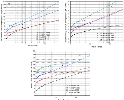
The Figure 8 shows the return level plots at different moments in different conditions: a) q= 0.6, b) q= 0.7 y c) q= 0.8. In this figure, it is possible to observe that there are changes in the form of the plots as a result of the changes in the shape parameters. These changes may affect the extrapolation due to sometimes the plot can be concave or convex. The dashed lines presented in the Figure 8 can help to determine the maximum pit depth value. In our example the Return Period value is 200.

1 10 100

0 2 4 6 8 10 12 14 16 18 20 22 24 26

10 years =-0.119 15 years =-0.065 20 years =0.019 25 years =0.109

R e tu rn L e ve l (Ma xi mu m p it d e p th in le n g th d e p th ) Retun Period a)

1 10 100

0 2 4 6 8 10 12 14 16 18 20 22 24 26

10 years =-0.099 15 years =0.003 20 years =0.096 25 years =0.051

Retu rn L ev el (M ax im um p it d ep th in le ng th d ep th ) Retun Period b)

1 10 100

0 2 4 6 8 10 12 14 16 18 20 22 24 26

10 years =-0.03 15 years =-0.025 20 years =0.096 25 years =-0.048

R e tu rn L e ve l (Ma xi mu m p it d e p th ) Retun Period c)

Figure 8. Return Level plot of the GEVD for: a) q = 0.6, b) q = 0.7 and c) q = 0.8. The dashed lines

can support to determine the maximum pit depth.

6. POT APPROACH

For the Peak-Over-Threshold approach We choose all the observations that exceed over a thresholdu. These observations are fitted to the Generalized Pareto Distribution (GPD) (See Equation (9)) [18] The Equation (9) is defined on x u y;





1/ *

( ) 1 1 x

H x        _{ } 

In order to approach using POT it is essential to select a thresholdu. This threshold can be selected using the mean residual plot and a sensitivity plot for the parameters * and . For the mean residual plot, the threshold selected must have a linear change. In the sensitivity plot the parameters must remain near-constant. The mathematical procedure for the plots already mentioned can be found in the Reference [18]. So as to choose the best threshold the package “POT” and “extRemes” were used.

As discussed in the last section, it is commonly opportune the use of quantiles or return levels. The quantiles can be obtained according to the Expressions (10) [18]









u T

u T

x u n

x u n

             (10)

Where nu is the number of observations after the thresholdu, A is the entire studied area and

aT is the total sample area.

100 101 102 103 0 2 4 6 8 10 12 14 16 18 20 22 24 26 28 30

10 years _{=-0.11 nu=37}

15 years _{=-0.04 nu=55}

20 years _{=0.06 nu=57}

25 years _{=0.17 nu=31}

Pi t d e p th u n its

Return Period n

u(A/aT)

A/aT=10

a)

100 ₁₀1 ₁₀2 ₁₀3

0 2 4 6 8 10 12 14 16 18 20 22 24 26 28 30

10 years _{=-0.11 nu=37}

15 years _{=-0.04 nu=55}

20 years _{=0.06 nu=57}

25 years _{=0.17 nu=31}

Pi t d e p th u n its

Return Period n_u(A/a_T)

A/aT=10

b)

100 ₁₀1 ₁₀2 ₁₀3

0 2 4 6 8 10 12 14 16 18 20 22 24 26 28 30

10 years _{=-0.11 nu=43} 15 years =-0.13 nu=43 20 years =-0.03 nu=41 25 years _{=-0.07 nu=132}

Pi t d e p th u n its

Return Period n_u(A/a_T)

A/aT=10

c)

Figure 9. Return Level plot of the GPD for: a) q = 0.6, b) q = 0.7 and c) q = 0.8. The dashed lines

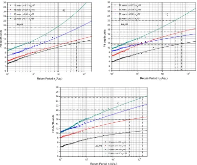
The data obtained in the last section were used again in order to know if there is any change in the shape parameter that can affect the extrapolation in the return period method. In the Figure 9, it is possible to observe how the shape parameter change in different times, like in the return level plots of the GEVD. It means that both GEVD and GPD can show the shape parameter evolution in time. To determine the extrapolated value of the maximum pit depth it is essential to know the number of observations that are greater than the chosen threshold (nu) and the A/aT ratio. The number of observations (nu) times the A/aT ratio defines the return period.

7. RESULTS AND DISCUSSIONS

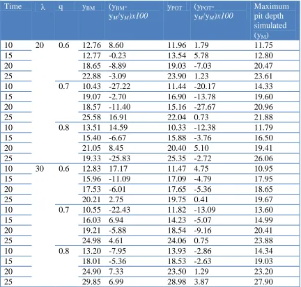
Table 1. Results obtained with the Block Maxima and Peak-Over-Threshold approaches.

Time  q yBM (yBM

-yM/yM)x100

yPOT (yPOT

-yM/yM)x100

Maximum pit depth simulated (yM)

10 20 0.6 12.76 8.60 11.96 1.79 11.75

15 12.77 -0.23 13.54 5.78 12.80

20 18.65 -8.89 19.03 -7.03 20.47

25 22.88 -3.09 23.90 1.23 23.61

10 0.7 10.43 -27.22 11.44 -20.17 14.33

15 19.07 -2.70 16.90 -13.78 19.60

20 18.57 -11.40 15.16 -27.67 20.96

25 25.58 16.91 22.04 0.73 21.88

10 0.8 13.51 14.59 10.33 -12.38 11.79

15 15.40 -6.67 15.88 -3.76 16.50

20 21.05 8.45 20.40 5.10 19.41

25 19.33 -25.83 25.35 -2.72 26.06

10 30 0.6 12.83 17.17 11.47 4.75 10.95

15 15.96 -11.09 17.09 -4.79 17.95

20 17.53 -6.01 17.65 -5.36 18.65

25 20.21 2.75 19.75 0.41 19.67

10 0.7 10.55 -22.43 11.82 -13.09 13.60

15 16.03 6.94 14.23 -5.07 14.99

20 19.21 -5.88 18.54 -9.16 20.41

25 24.98 4.61 24.06 0.75 23.88

10 0.8 13.20 -7.95 13.93 -2.86 14.34

15 18.01 -5.36 18.53 -2.63 19.03

20 24.90 7.33 23.50 1.29 23.20

25 29.85 6.99 28.98 3.87 27.90

obtained in the simulations. The percentage of error respect to the maximum value is also shown in the fifth and seventh column for BM and POT respectively.

In the Table 1 can notice that the POT is the best approach in 20 cases from the total of 24. It means that using this approach in situations where it is not possible to inspect a large percentage of the area. Usually the POT approach is not a well-known method in pressure vessels integrity engineering because of the higher mathematical complexity in comparison with the Block Maxima, BM. However, according to the results presented in this paper, the use of GPD in the maximum pit depth extrapolation can be reliable because describe the physical behavior of the maximum pit depth. As it was mentioned before, the shape parameter increases in time. This change is attributed to the new pits that have a different growth rate respect to the older pits and also to the fact that the deeper pits that also have a different rate respect to others.

Taking into account the shape evolution time in the extrapolation, it feasible to increase the accuracy in the estimation and therefore reduce the number of inspections. This can help in manage better the risk in the pressure vessels.

In the oil industry, it is difficult to inspect an entire vessel with a non-destructive test (NDT), for that reason the vessel could be inspected in only some parts. The results of the inspection are used to determine if the vessel is reliable to keep working. Therefore, it is necessary to use all the statistical methods and its understanding in the data analysis. BM is a widely used method but it is more conservative, it means that applying this method can provoke unnecessary repairs.

In order to motivate people interested in applying their mathematics knowledge in pitting corrosion modeling, Velázquez and coworkers published field data information in the Reference [25]. This has the goal of being able to understand better the stochastic nature of the phenomenon.

8. CONCLUSIONS

The use of statistical simulations in the pitting corrosion is useful to know the different characteristics of the phenomenon described below.

First of all, despite the pit initiation time is a key factor to determine the structural deterioration, there is no practical engineering technique capable to measure it. Describing as a Non Homogeneous Possion Process, one can determined the evolution of the total number of pits.

Second, the pitting growth has a stochastic behavior. This behavior can be perfectly described by the Gamma Process because the mean and variance have a well recognized evolution. This process is also very useful because of the capacity to couple successfully the stochastic attribute of the pitting initiation and the pitting growth. Also, it is feasible to consider the non-linear characteristic of the pitting growth.

The extrapolation methods also repeat the time evolution of the shape parameter that is regularly presented in the maximum pit depth distributions. Another point to conclude it is that POT approach estimates in a better way the maximum pitting corrosion depth than the BM approach.

ACKNOWLEDGEMENTS

like to thanks Sistemas Automatizados e Industriales S.A. de C.V. for its financial and materials support.

References

1. http://www.corrosion.org/images_index/nowisthetime.pdf 2. http://nvl.nist.gov/pub/nistpubs/jres/115/5/V115.N05.A05.pdf.

3. http://www.oildompublishing.com/pgj/pgjarchive/March03/corrosioncosts3-03.pdf. 4. htpp://primis.phmsa.dot.gov/comm/reports/safety/sida.html?nocache=6853.

5. F. Caleyo, L. Alfonso, J. Alcántara and J.M. Hallen, ASME J. of Pressure Vessels Technology, 130 (2008) 021704/1–021704/8.

6. Seventh EGIG-report 1970–2007, Gas Pipeline Incidents, Doc. No. EGIG08.TV-B.0502, December 2008.

7. http://www.esmap.org/esmap/sites/esmap.org/files/03403RussiaPipelineOilSpillStudyAppendix.pd f

8. P.M. Aziz, Corrosion 12 (1956) 495t-506t.

9. M. Nessin, “Estimating the risk of pipeline failure due to corrosion”, W. Revie, Editor, Uhlig’s Corrosion Handbook, 2nd Edition, John Wiley & Sons, Inc. (2000) pp. 85.

10. M. Romanoff, Underground corrosion, NBS Circular 579, National Bureau of Standard, Washington, DC (1957).

11. Y. Katano, K. Miyata, H. Shimizu and T. Isogai, Corrosion 59 (2003) 155–161. 12. J.C. Velazquez, F. Caleyo, A. Valor and J.M. Hallen, Corrosion 65 (2009) 332–342

13. A. Valor, F. Caleyo, L. Alfonso, D. Rivas and J.M. Hallen, Corrosion Sci. 49 (2007) 559–579. 14. F. Caleyo, J.C. Velázquez, A. Valor and J.M. Hallen, Corrosion Sci. 51 (2009) 2197–2207. 15. F. Caleyo, J.C. Velázquez, A. Valor and J.M. Hallen, Corrosion Sci. 51 (2009) 1925–1934 16. L. Alfonso, F. Caleyo, J.M. Hallen and J. Araujo, “On the Applicability of Extreme Value

Statistics in the Prediction of Maximum Pit Depth in Heavily Corroded Non-Piggable Buried Pipelines”, 8th International Pipeline Conference (IPC2010) September 27–October 1, 2010 , Calgary, Alberta, Canada, IPC2010-31321, pp. 527-535

17. M. Kowaka, Introduction to Life Prediction of Industrial Plant Materials: Application of the Extreme Value Statistical Method for Corrosion Analysis, Allerton Press, Inc., New York (1994), pp. 30.

18. S. Coles, An Introduction to Statistical Modeling of Extreme Values, Springer Series in Statistics, Springer-Verlag, London, UK (2001) pp. 47.

19. J. M. van Noortwijk and Dan M. Frangopol, Probabilistic Engineering Mechanics, 19 (2004) 345-359.

20. V. G. Kulkarni, Modeling and analysis of stochastic systems, Chapman and Hall, London, UK, First Edition, 1995, pp. 208-210.

21. S. P. Kuniewski , J.A.M. van der Weide and J. M. van Noortwijk, Reliability Engineering & System Safety, 94 (2009) 1480-1490

22. J.W. Provan and E.S. Rodríguez, Corrosion 45 (1989) 178.

23. J.M. van Noortwijk, Reliability Engineering & System Safety, 94 (2009) 2-21

24. E. Castillo, Extreme Value Theory in Engineering, Academic Press, Inc., San Diego (1988), pp. 55 25. JC Velázquez, F Caleyo, A Valor, JM Hallen, Corrosion, 66 (2010) 016001-016001-5.