https://doi.org/10.1007/s10955-018-2146-2
Minority Population in the One-Dimensional Schelling Model
of Segregation
George Barmpalias1·Richard Elwes2 ·Andrew Lewis-Pye3
Received: 14 March 2018 / Accepted: 29 August 2018 / Published online: 6 September 2018 © The Author(s) 2018
Abstract
Schelling models of segregation attempt to explain how a population of agents or particles of two types may organise itself into large homogeneous clusters. They can be seen as variants of the Ising model. While such models have been extensively studied, unperturbed (or noiseless) versions have largely resisted rigorous analysis, with most results in the literature pertaining models in which noise is introduced, so as to make them amenable to standard techniques from statistical mechanics or stochastic evolutionary game theory. We rigorously analyse the one-dimensional version of the model in which one of the two types is in the minority, and establish various forms of threshold behaviour. Our results are in sharp contrast with the case when the distribution of the two types is uniform (i.e. each agent has equal chance of being of each type in the initial configuration), which was studied in Brandt et al. (in: STOC ’12: proceedings of the 44th symposium on theory of computing, pp. 789–804,2012) and Barmpalias et al. (in: 55th Annual IEEE symposium on foundations of computer science, Oct 18–21, Philadelphia, FOCS’14,2014).
Keywords Schelling segregation·Minority population·Phase diagram
1 Introduction
The economist Thomas Schelling introduced his model of segregation in [30] (developed later in [28,29]), with the explicit intention of explaining the phenomenon of racial segregation
B
Richard Elwes [email protected]George Barmpalias [email protected]
Andrew Lewis-Pye [email protected]
1 State Key Lab of Computer Science, Institute of Software, Chinese Academy of Sciences, Beijing,
China
2 School of Mathematics, University of Leeds, Leeds LS2 9JT, UK
3 Department of Mathematics, London School of Economics, Columbia House, Houghton Street,
in large cities. Perhaps the earliest agent-based model studied by economists, since then it has become an archetype of agent-based modelling, prominently featuring in libraries of modelling software tools such as NetLogo [35] and often being the subject of experimental analysis and simulations in the modeling and AI communities [11,12,15,16,18,19,21,32,36]. Many versions of the model have been analysed theoretically, from a number of different viewpoints and disciplines: statistical mechanics [8,14] and [4, Sect. 3.1], evolutionary game theory [37–40] the social sciences [9,10,27], and more recently computer science and AI [1,5,
7,13]. It was observed in [7], however, that despite the vast amount of work that has been done on the Schelling model in the last 40 years, rigorous mathematical analyses in the previous literature generally concern altered versions of the model, in which noise is introduced in the dynamics, i.e. where one allows that agents may make non-rational decisions that are detrimental to their welfare with small probability. The introduction of such ‘perturbations’ may be justifiable from a ‘bounded rationality’ standpoint.
The model (which will be formally defined shortly) concerns a population of agents arranged geographically, each being of one of two types. Each agent has a certain neighbour-hood around them that they are concerned with, and also an intolerance parameterτ ∈ [0,1] which we shall assume here to be the same for all agents. An agent’s behaviour is dictated by the proportion of the agents in their neighbourhood which are of its own type. So long as this proportion is≥τ the agent may be considered ‘happy’ and will not move. Starting with a random configuration, one then considers a discrete time dynamical process. At each stage unhappy agents may be given the opportunity to move, swapping positions with another agent, so as to increase the proportion of their own type within their neighbourhood. Now one might justify a perturbed version of these dynamics, in which agents will occasionally move in such a way as to decrease their utility (i.e. the proportion of their own type within their neighbourhood) by arguing, for example, that it is reasonable to suppose that only incomplete information about the make-up of each neighbourhood is available to the agents. It is a fact, however, that
(a) the methods used for the analysis of the perturbed models do not apply to the unperturbed model;
(b) the segregation occurring in the perturbed models is very different than in the unperturbed model.
In the unperturbed models the underlying Markov chain does not have the regularities that are found in the perturbed case (e.g. the Markov process is irreversible). The presence of a large variety of absorbing states means that entirely different and more combinatorial methods are now required. Beyond the basic aim of a rigorous analysis for these unperturbed models, which have been so extensively studied via simulations, further motivation is provided by the fact that the Schelling model is part of a large family of models, arising in a broad variety of contexts—spin glass models, Hopfield nets, cascading phenomena as studied by those in the networks community—all of which aim at understanding the discrete time dynamics of competing populations on underlying network structures of one kind or another, and for many of which the unperturbed dynamics are of significant interest. The hope is that techniques developed in analysing unperturbed Schelling segregation may pave the way for similar analyses in these variants of the model.
Table 1 Parameters of the
Schelling model Parameter Symbol Range
Population n N
Neighbourhood radius w [0,n] Tolerance threshold τ [0,1] Expected/actual minority proportion ρ/ρ∗ [0,1]
and population. More significantly, however, it dealt only with the symmetric case where intolerance parameterτ =0.5 (i.e. an agent is happy when at least 50% of the agents in its neighbourhood are of its own type). In [1] a much more general analysis of the unperturbed one-dimensional Schelling model forτ ∈ [0,1]was provided. In fact it was shown there that various forms of surprising threshold behaviour exist. A significant symmetry assumption underlying the results in [1,7] is that the populations of the two types of agents are assumed to be uniform (i.e. each agent has equal chance of being of each type in the initial configu-ration). Indeed, there is no rigorous study of the unperturbed spacial proximity model with swapping agents for the rather realistic case where the distribution of the two types of agents is skewed. In fact, the question as to what type of segregation occurs with a skewed population distribution was raised by Brandt et al. in [7, Sect. 4] as well as in popular expositions of the Schelling model like [20].
The purpose of the present work is to give an answer to this question. We show that complete segregation is the likely outcome if and only if the intolerance parameter is larger than 0.5. Moreover in the case that the minority type is at most 25%, there is a dichotomy between complete segregation and almost complete absence of segregation.
1.1 Definition of the Model
Schelling’s model of residential segregation belongs to a large family of agent-based models, where a system of competitive agents perform actions in order to increase their personal welfare, while possibly decreasing the welfare of other individuals. This phenomenon roughly corresponds to the so-calledspontaneous order approach1 in economics literature, which studies the emergence of norms from the endogenous agreements among rational individuals. The Schelling model that we study is a direct generalisation of that in [7] and also that studied by the authors in [1]. The one-dimensional model with parametersn, w, τ, ρ(as listed in Table1) is defined as follows. We considernindividuals which occupy an equal number ofsites0, . . . ,n−1 (ordered clockwise) on a circle. Each of the individuals belongs to one of the two typesαandβ. The type assignment of individuals is independent and identically distributed (i.i.d.), with each individual having probabilityρof being typeβ. Without loss of generality we always assume thatρ≤0.5, i.e. that the individuals of typeβare the expected minority (so long asρ =0.5). This random type assignment takes place at stage 0 of the process, and defines theinitial state. At the end of stage 0, we letρ∗be theactualproportion of the individuals that are of typeβ (i.e.ρ∗is the random proportion, as opposed to the expected proportionρ).
Unless stated otherwise, addition and subtraction on indices for sites are performed modulo n. Given two sitesu, vin any configuration of the individuals on the circle, the interval[u, v]
1This contrasts themechanism design approachwhich studies the exogenous (a priori) design of regulations
consists of the individuals that occupy sites betweenu andv (inclusive). For example, if 0≤v <u<nthen we let[u, v]denote the set of nodes[u,n−1] ∪ [0, v](while[v,u]is, of course, understood in the standard way). When we talk about a particular configuration, we identify each individual with the site it occupies, referring to both entities as anode. The neighbourhoodof nodeuconsists of the interval[(u−w), (u+w)]wherewis a parameter of the model that we call the (neighbourhood)radius. Thetolerance thresholdτ ∈(0,1)is another parameter of the model that reflects how tolerant a node is to nodes of different a type in its neighbourhood. We say that a node ishappyif the proportion of the nodes in its neighbourhood which are of its own type is at leastτ.
Given the initial type assignment (colouring) of the nodes, theSchelling processthen evolves dynamically in stages as follows. At each stages>0 we pick uniformly at random a pair of unhappy nodes of different type, and we swap them provided that in both cases the number of nodes of the same type in the new neighbourhood is at least that in the original neighbourhood. If at some stage there are no further legal swaps the process terminates. If at some stage all nodes of the same type are grouped into a single block (i.e. a contiguous interval), we say that at that stage we havecomplete segregation.
This completes the definition of the Schelling process with parametersn, w, τ andρ, which we denote by the tuple(n, w, τ, ρ). The process can be seen as a Markov chain with 2n states corresponding to the configurations that we get by varying the type of each node
betweenαandβ. A state is calleddormantif either allα-nodes are happy, or allβ-nodes are happy. We shall be interested in the case thatw is large, and thatnis large compared tow. In this context it will turn out that the absorbing states of the Schelling process are exactly the dormant states and, in fact, the only recurrence classes of the Schelling process are the dormant states and complete segregation. Complete segregation is, strictly speaking, a recurrence class of the process, consisting of the rotations of the two blocks, one consisting of all theα-nodes and the other consisting of all theβ-nodes. Hence, modulo symmetries, we may regard complete segregation as an absorbing state. Dormant states are a different kind of absorbing state, as the process actually stops when it hits a dormant state. Note that a static process cannot come to complete segregation, since it does not allow a sufficient number of swaps for the complete separation of the node types on the ring to be formed, starting from a random state. Note that the number of nodes of typeαand of typeβdoes not change between transitions, once the initial state has been chosen.
1.2 Our Results
Given the Schelling process(n, w, τ, ρ)we wish to determine with high probability the type of equilibrium that will eventually occur in the system. Given a constantc≥0, we write ‘for cwn’, to mean ‘for allwsufficiently large compared toc, and allnsufficiently large compared tow’; formally, we say that a result with parametersw,nholds forcwn, if there exist functionsc →Wc,w → Nwsuch that the result holds for eachw > Wcand
n≥Nw. We are interested in asymptotic results, i.e. statements that hold with arbitrarily high probability for 0w n. The following definition encapsulates the type of asymptotic statements about the Schelling process(n, w, τ, ρ)that we are interested in establishing.
(n, w, τ, ρ)is static if, given > 0, with high probability the number of nodes that ever change their type in the entire duration of the process is≤·n.2
By [1,7], the asymptotic behaviour of the process (n, w, τ, ρ)is known for ρ = 0.5 (except on the thresholdτ =κ0 ≈0.353). The present work is dedicated to the case where one type of node is the minority, i.e. whenρ < 0.5. We show that with probability 1 the process will either reach complete segregation or reach a dormant state. Moreover we show that whenτ >0.5 the highly probable outcome is complete segregation. Moreover, in many cases whenτ ≤ 0.5 the outcome is negligible segregation (i.e. the process is static). Let κ0 ≈0.353 andλ0 ≈0.4115 be the unique solutions of(0.5−x)0.5−x =(1−x)1−x and 2τ·(0.5−τ)1−2τ =(1−τ)2(1−τ)respectively in[0,0.5].3
Theorem 1 (Main result)Ifτ >0.5,ρ <0.5andτ+ρ=1, then with high probability the Schelling process(n, w, τ, ρ)reaches complete segregation. The process is static (with high probability) if
[τ ≤λ0&ρ≤λ0] or [τ ≤κ0&ρ <0.5] or [τ ≤0.5 &ρ≤0.25]
or, more generally, if2ρ·(1−2κ0)+τ+κ0<1.4
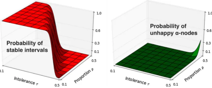
The values of (τ, ρ) for which we show that the process is static, correspond to the triangular area of the first diagram (or, equivalently, the collapsed part of the surface of the third diagram) of Fig.1. The case whenρ≤0.25 presents a remarkable contrast asτcrosses the boundary of 0.5. In this case, whenτexceeds the threshold 0.5, the process changes from static to the other extreme of complete segregation.
Corollary 1 (Phase transition on 0.5)Ifρ ≤ 0.25, then with high probability the process (n, w, τ, ρ)
– converges to complete segregation ifτ >0.5; – is static, ifτ≤0.5.
Moreover with high probability it reaches its final state in timeon, ifτ ≤ 0.5and time Ω(n), ifτ >0.5.
We display these results in Table2. In Sects.2–4we present the argument that proves these results. This argument uses a number of smaller results which are stated without proof, and are the building blocks of the proof of Theorem1. It is our intention that the reader gets a fairly good understanding of our analysis in this part of the paper, without the burden of having to verify some of the more technical parts of the proof. Sect.5contains the detailed proofs of all the facts that were used in Sects.2–4, and completes the proofs of Theorem1
and Corollary1.
2In other words, we say that the process(n, w, τ, ρ)is static if throughout the process (which could potentially
take infinitely many steps) the number of nodes that ever change their type is an arbitrarily small proportion of the entire population—tends to 0 with probability tending to 1 as n tends to infinity. In Sect.4.2we will show that this definition is equivalent to requiring that with high probability the duration of the process in steps is an arbitrarily small proportion ofn, in the same sense.
3At this point, the constantsκ
0, λ0are simply the solutions of the above equations. These equations are
generated by comparing certain distributions in the limit, as will become clear in the technical sections of this article.
4The first three conditions are special cases of the latter inequality—see the first item of Fig.1for an
Fig. 1 Threshold behaviour whenτ, ρare in[0,0.5]. The two-dimensional axes refer toτandρ. In the first figure, the process is static except for the(τ, ρ)in the small area at the top right corner. The second figure is a plot ofPstabandPunhap(for w = 100) as functions of(τ, ρ). The third figure is a plot ofg(τ, ρ)for w = 100
Table 2 The main result Process parameters Segregation
τ < λ0 & ρ < λ0 Negligible
τ≤κ0 & ρ <0.5 Negligible
τ≤0.5 & ρ≤0.25 Negligible
τ >0.5 & ρ≤0.5 Complete
Table 3 Two cases for the process(n, w, τ, ρ)and the corresponding expectations of the number of initially happy nodes
Case Condition Happyα Happyβ
Balanced happiness τ+ρ >1,τ >0.5 n·e−Θ(w) n·e−Θ(w) Unbalanced happiness τ+ρ <1,τ >0.5 n·1−e−Θ(w) n·e−Θ(w)
Our proof of Theorem1is nonuniform, and the analysis is roughly divided in the two cases displayed in Table3:balanced happiness(whenτ+ρ >1,τ >0.5) andunbalanced happiness(whenτ +ρ < 1,τ >0.5). Herehappinessrefers to the numbers of initially happy nodes of the two types, and determines the dynamics that drives the process to an equilibrium. Of the two cases,unbalanced happinessis the most challenging to deal with, and the dynamics is driven by a small number of unhappyα-nodes against the large number of unhappyβ-nodes, which in fact is preserved throughout a significant part of the process.
1.3 Schelling Models and Relation to Spin-1 Physical Models
[image:6.439.166.393.187.257.2] [image:6.439.46.393.297.348.2]such as the Schelling model. Although similar models but with ‘short-range’ interactions have been studied in the past, e.g. [17], rigorous results for the corresponding models with “long-range” interactions are currently under study.
Numerous authors, for example [14,23,25,26,34], have noted the close relationship between Schelling models and variants of the Ising Model, widely studied by statistical physicists to understand phase transitions. In this situation, perturbed or noisy versions of the model correspond to a temperatureT > 0, which can productively be analysed using the Boltzmann distribution. Typically the limitT → 0 is then studied. Thus the current work can be viewed as a study of a family of 1-dimensional kinetic Ising models with range of interactionw, as non-equilibrium systems under rapid cooling, that is atT = 0 (where radically different behaviour can be observed than in the limitT →0). In this situation, the Boltzmann distribution is no longer a viable tool, and the use of the thresholdτcan be seen as a simple alternative in determining whether or not a spin will update if selected.
In the current work, the model evolves by swapping pairs of agents of opposite types, cor-responding to “closed” spin-1 systems underKawasaki dynamicsin which magnetization is conserved (and which are used to model alloy systems), whereas versions such as [2] in which individual agents switch type correspond to “open” spin-1 systems underGlauber dynamics in which magnetization is not conserved. To make the connection explicit, (temporarily) writeSi(t)= +1(respectively−1)if siteiis occupied by a node of typeα(respectivelyβ)
at timet. Then the spin at siteiis unhappy (and thus willing to swap) if and only if
j:|j−i|≤w
SiSj−(2τ−1)(2w+1)
<0.
In our view, it is the simplicity of the original Schelling model, contrasted by the complexity of the analysis required to specify its behaviour, as demonstrated in [1,7] and the present work, that make this topic fundamental and interesting. Under the above requirement for simplicity and proximity to the original model, there remain a number of ways that the model can be altered or generalised. For example, note that in the case thatτ >0.5 in the model of Sect.1.1, two nodes may swap although the number of same-type nodes in their neighbourhoods remain the same after the swap. One may alternatively require that for such a swap, the corresponding numbers of same-type nodes in the neighbourhoods increase (note that such a modification would not make a difference ifτ ≤0.5). Our choice on this issue follows Brandt et al. in [7, §2]. One generalisation, considered in [2], is to allow different tolerance thresholds for the two types of individuals. Another generalization, already present in [30], is to introduce a number of vacancies, i.e. to allow the total number of individuals to be smaller than the number of sites.
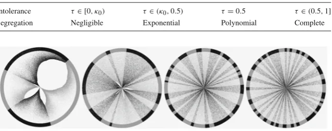
Table 4 Segregation regions in the caseρ=0.5
Intolerance τ∈ [0, κ0) τ∈(κ0,0.5) τ=0.5 τ∈(0.5,1]
Segregation Negligible Exponential Polynomial Complete
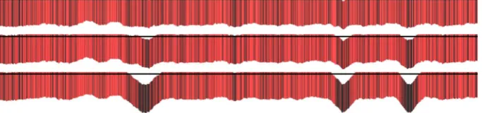
Fig. 2 500K population withw=3000, ρ =0.5 andτ =0.485,0.49,0.495,0.5. All made about 130K swaps
1.4 Objectives of the Analysis of the Unperturbed Model and Related Work
We use the notation of Sect.1.1, so that the symbolnalways means the population variable of the process, andwalways is the parameter of the process which determines the length of the neighbourhood of nodes. Similarly,τ, ρalways refer to the parameters of the Schelling process.
In Sect.2.2.3we show that, with probability one, the process(n, w, τ, ρ)either reaches complete segregation or it reaches a dormant state. In the second case, we wish to determine the extent of segregation in the dormant state. In view of the large number of states that the process may have (most of them ‘random’) a question arrises as to how to classify or even talk precisely about different states that may be the outcome of the process. Brandt et al. noticed in [7] that, at least in the caseτ =ρ=0.5 that they considered, the extent of the segregation that occurs in the final state depends crucially onw. In fact, they showed that the dependence onwis at most ‘polynomial’. We may say that a state is regarded aspolynomial segregationif, with high probability a randomly chosen node belongs to a contiguous block5 of size that is proportional to the value of a polynomial onw. A similar definition applies toexponential segregation. These two notions turn out to provide a very useful language for explaining the eventual outcome of the Schelling process. A full characterization (extending the work of Brandt, Immorlica, Kamath, and Kleinberg [7]) of the asymptotic behaviour of the process(n, w, τ, ρ)forρ =0.5 andτ ∈ [0,1]was provided by the authors in [1] in terms of polynomial and exponential segregation, as well as static processes. Intuitively, a random state is non-segregated, while polynomial and exponential segregation correspond to highly non-random states.
The characterization from [1] is summarized in Table4. It is rather striking that when intolerance is increased from, say, 0.4–0.5 the segregation is decreased. This phenomenon is akin to the many paradoxes that stem from the missing link between local motives of agents and global behaviour of a system (e.g. see Schelling’s classic monograph [31], and in particular Chapter 4 which relates to his segregation models). Even more strikingly, the authors showed in [1] that the paradox occurs for allτ ∈(κ0,0.5), i.e. asτ approaches 0.5 the segregation (in the final state) decreases.
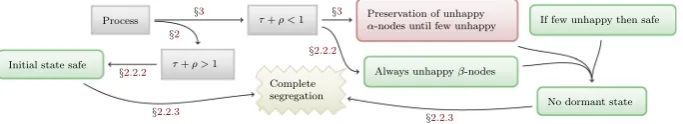
If few unhappy then safe
No dormant state Preservation of unhappy
α-nodes until few unhappy
τ+ρ <1
Initial state safe
Always unhappyβ-nodes Process
τ+ρ >1
Complete segregation §2
§2.2.2 §3
§2.2.2 §3
§2.2.3 §2.2.3
Fig. 3 The logic of the proof that ifτ >0.5, with high probability the process reaches complete segregation
This paradoxical phenomenon is also clear in many simulations of the model. Figure2
shows typical runs of the processes(5×105,3×103, τ,0.5)forτ ∈ {0.485,0.49,0.495,0.5}. The final state is depicted in the circle, where the nodes of one type are black and the nodes of the other type are grey. We use the space between the centre of the ring and the ring in order to record the actual process, as it evolves in time. In particular, if a grey node switches its place with a black node, we put a black node (the colour of the more recent node) between the location of the node and the centre of the ring, at a distance from the centre which is proportional to the stage where the swap occurred. Hence we may observe “cascades’ of swaps of nodes of the same type, which are less severe asτ approaches 0.5. Such cascades are crucial in the rigorous analysis of the model, both in [7] and in [1]. Figure2shows that asτ approaches 0.5, the segregation is decreased. This behaviour can be traced to the probability that a node is unhappy in the initial configuration, and in fact, the threshold constantκ0is derived by comparing related probabilities in [1].
In the caseρ=0.5 the two constantsκ0and 0.5 markphase transitionsin the limit state of the process(n, w, τ, ρ), asτ takes values in[0,1]. This brings us to another important objective of the analysis of the Schelling process, which is the discovery of phase transitions with respect to the parametersτ, ρ. Incidentally, we note that the discovery of phase transitions has been one of the original motivations for the study of the one and two dimensional Ising model, when one varies the temperature (see the end of Sect.1.3for a brief discussion of the analogy between the Ising and the Schelling models). Finally we are also interested in the expected time that the process takes to converge.
1.5 Overview of Our Analysis
We use different methods for the casesτ ≤ 0.5 (Sect.4) andτ >0.5 (Sects.2and3). If τ ≤ 0.5, in order to derive conditions under which the process is static, we analyse and compare the probabilities of initially unhappy nodes andstable intervals.6 Ifτ >0.5 we consider the two casesτ+ρ <1 (Sect.3) andτ+ρ >1 (Sect.2) and argue (using distinct arguments) that in each of them complete segregation is the high probability outcome.
Caseτ>0.5This case is divided to the casesτ+ρ >1 andτ+ρ <1, and the structure of the analysis is depicted as a flowchart in Fig.3(along with the sections where the various implications are analysed), and in more detail in Fig.4. First, we show that asymptotically (onw,n), from any state there is a series of transitions that leads to either a dormant state, or complete segregation. Hence, since there are only finitely many states, with probability one the process will reach either a dormant state or complete segregation. So in order to establish complete segregation as the eventual outcome, it suffices to show that the process maintains unhappy nodes of each colour during all stages.
6Stable intervals are, roughly speaking, intervals of nodes that do not allow the spread of unhappyα-nodes
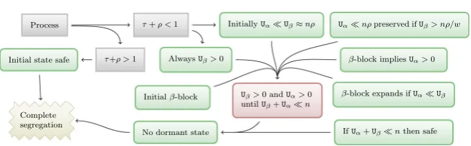
[image:9.439.51.393.57.119.2]Uαnρpreserved ifUβ> nρ/w
β-block impliesUα>0
Initialβ-block β-block expands ifUαUβ
IfUα+Uβnthen safe
Uβ>0 andUα>0 untilUβ+Uαn InitiallyUαUβ≈nρ
τ+ρ <1
Initial state safe AlwaysUβ>0 Process
τ+ρ >1
Complete segregation
No dormant state
Fig. 4 The logic of the proof that ifτ >0.5, with high probability the process reaches complete segregation. Here ‘β-block’ refers to the persistentβ-block of Sect.3.1
First, assume thatτ +ρ >1, a case which is dealt with in Sect.2. In this case we can show in Sect.2.2.3that, assuming that the actual proportion ofβ-nodes is sufficiently close toρ (which is very likely according to the law of large numbers), every reachable state is not dormant. More precisely, we show that given such numbers ofαandβ-nodes, every permutation of them on the ring corresponds to a state which has both unhappyαand unhappy β-nodes. Since the numbers of nodes of each type do not change during each transition, this argument suffices for this case. States with the property that no series of transitions from them leads to dormant states are calledsafe. So, in the caseτ+ρ >1 we argue that (with high probability) the initial state is safe.
Second, we assume thatτ+ρ <1, which is a considerably harder case that we deal with in Sect.3. Under this hypothesis, in the initial configuration we haveonmany unhappy α-nodes andΩ(n)many unhappyβ-nodes. As before, it suffices to show that (with high probability) the process never reaches a dormant state. It is not hard to see that (with high probability) the initial state is not dormant. However it is no longer clear if the initial state is safe. In Sect.2we show that given the expected numbers of nodes of the two types in the initial state (or numbers sufficiently close to their expectations) any permutation of the nodes on a ring corresponds to a state with at least one unhappyβ-node. Hence, with high probability, the process will never run-out of unhappyβ-nodes and we only need to argue about the preservation of unhappyα-nodes. Already it should be clear that this is anasymmetriccase where theα-nodes (the majority) and theβ-nodes (the minority) play different roles. When τ+ρ <1 there are many permutations of the nodes (which correspond to states where all α-nodes are happy, i.e. dormant states. So the argument that was used in the caseτ+ρ >1 is no longer relevant for arguing for the preservation of unhappyα-nodes in the process. The argument we use instead (technically overviewed in Sect.3.2and executed in Sects.3.3,3.4) is based on the asymmetry between the number of unhappyβ-nodes and the unhappyα-nodes, which creates a dynamic that favours the preservation of unhappyα-nodes. More precisely, it favours the preservation ofβ-blocks of length> w, which is a condition implying the existence of unhappyα-nodes (indeed, theα-nodes neighbouring aβ-block of length at least ware unhappy). Hence if we show that the expected number of unhappyα-nodes remains small during the stages of the process, then we can expect the existence of unhappyα-nodes (and unhappyβ-nodes) up to the point where the total number of unhappy nodes is small.
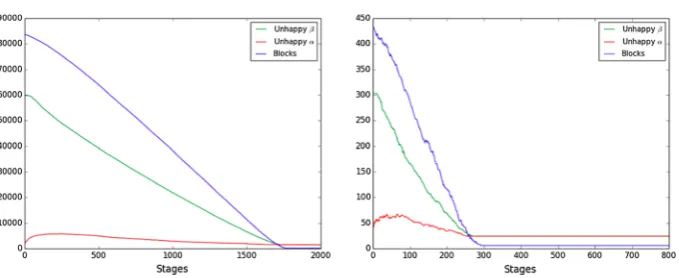
[image:10.439.50.391.47.153.2]-Fig. 5 The first plot is from the process(200,000,50,0.6,0.3) and the second one from the process
(1000,20,0.6,0.3). These simulations illustrate that the numberα-nodes in the infected area remains bounded, until the number ofβ-nodes outside the infected area becomes small. The second figure also illustrates the fact that the number of unhappy nodes fluctuates locally
node during the stages, taken from two typical simulations (one with large and one with small population), whenτ+ρ <1.7The process we described is clearly visible: the number of unhappyα-nodes remains small, until the number of unhappyβ-nodes becomes small. Up to the later point, as we explained, the dynamics favours the preservation of unhappyα-nodes.
Caseτ ≤0.5In this case, dealt with in Sect.4, we haveτ +ρ < 1, and this means that in the initial configuration theα-population is happy with a few exceptions, while theβ -population is unhappy, with a few exceptions. Recall that in this case we wish to show that the process is static. By the definition of the dynamics of the modelα-to-βswaps can only occur in areas where there are unhappyα-nodes. Hence in this case theα-to-β swaps will be concentrated in a very few selected areas in the ring, at least in the first stages of the process. This concentration ofα-to-βswaps creates cascades ofα-node evictions which can be clearly seen in simulations such as the one displayed in Fig.6.8 If we could argue that such cascades are restricted to small areas around the initially unhappyα-nodes, then it is not hard to argue that the process reaches a dormant state rather quickly, having affected only a very small number of nodes. The way we do this is throughstable intervals, a device that was also used in [1]. Roughly speaking, these are intervals that do not allow the spread of unhappyα-nodes through them.
Ifρis very small, or ifτis very small, then stable intervals occur with high probability. On the other hand, ifρ, τ get sufficiently large, the probability of a stable interval tends to 0 asw→ ∞. This contrasts with prevalence of unhappyα-nodes. Whenτ, ρare small, the probability of (the occurrence of) an unhappyα-node is small, while it gets large whenτ, ρ increase. Figure7shows the actual probabilities (as calculated in Sect.4) as functions ofτ, ρ for the specific value ofw = 100 (the shape of the plots does not change significantly for different values ofw). The interesting case is the range forτ, ρwhere both probabilities tend to 0 asw→ ∞, i.e. both events become rare. Somewhere on the horizontalτ-ρplane there is a line marking the intersection of the two surfaces. This is where the probability of a stable
7Roughly speaking, theinfected areaincludes the parts of the ring which contain unhappyα-nodes; a formal
definition is given in Sect.3.2.
8Here the current configuration is the outer circle, while the initial random state is the inner small circle.
[image:11.439.51.391.49.188.2]Fig. 6 The evolution of the infected area whenτ+ρ <1. The current state in the outer circle, the initial state is in the inner circle, and each move of anα-node is represented by a dot at the coordinates of the new position, but at a distance from the center which is proportional to the stage where the swap occurred. This representation of the process in time illustrates the cascades of swaps that occur and start from the initial unhappyα-nodes
Fig. 7 The probabilities of a stable interval and an unhappyα-node, as functions ofτ, ρ≤0.5 whenw=100
interval becomes less than the probability of an unhappyα-node. Moreover, asw→ ∞the ratio of the two probabilities tends to infinity or zero, depending whetherτ, ρsit on one side of the plain (with respect to the intersection line) or the other. The crux of the argument in Sect.4is that for many values ofτ, ρstable intervals are much more common than unhappy α-nodes in the initial configuration. This allows us to argue that, in this case, the process has to reach a dormant state afteronmany swaps, which implies that the process is static.
1.6 Probability Terminology and Asymptotic Notation
In Sect.5.1we summarize some facts from probability theory that are used in our analysis. In Sect.5.2we state and prove some basic probabilistic facts about the Schelling model, which are also needed in our analysis. Asymptotic notation will be useful in expressing various statements in our analysis. We already defined the notation 0wnin Sect.1.2. Given two functions f,gon the positive integers, (as is standard) we say that f isOgif there exists a positive constantcsuch that f(t)≤c·g(t)for allt. We say thatgisΩ(f)if f isOg, and thatgisΘ(f)if both f isOgand f isΩ(g). We also use this notation, however, in a more general sense: we say that f isg(Ot)if there exists somec>0 such
that f ≤g(ct)for allt. For example, when we say that a function f isne−O
t, this means
that there isc >0 such that f(t)≤ne−ctfor allt. Or, if we say that f isn(1−e−O
[image:12.439.58.390.47.138.2] [image:12.439.51.389.202.343.2]this means that there isc>0 such that f(t)≤n(1−e−ct)for allt. Similarly, we useΘin a more general sense. We say that f isg(Θ(t))to mean that there exist constantsc0andc1 such thatg(c0·t)≤ f(t)≤g(c1·t)for allt. We say that f =o
gif limt f(t)/g(t)=0.
The (often hidden) variable underlying the asymptotic notation in the various expressions will bew. In other words, for fixed values ofρandτ, the choice of constants required in the asymptotic notation, will always depend only onw. We also combine the ‘high probability’ terminology with the asymptotic notation in a manner which is worth clarifying. When we say, for example, that ‘with high probability the number of initially unhappyα-nodes in the process(n, w, τ, ρ)is n·(1−ρ)·e−Θ(w)’, this means that there exist constantsc0 and c1such that, with high probability, the number of initially unhappyα-nodes in the process (n, w, τ, ρ)lies betweenn·(1−ρ)·e−c0·wandn·(1−ρ)·e−c1·w.
2 Metrics and Reaching Complete Segregation (
>
0
.
5
,
+
>
1)
One of the most challenging problems in the analysis of the segregation process is the large number of absorbing states. In order to understand which transitions are possible, we use certain metrics that describe the current state.
2.1 Welfare, Mixing, and Expectations
We define global metrics that reflect the welfare of the entire population.9These metrics and their properties are essential in all of the proofs that will follow. An obvious choice is the number of happy nodes at a given state. It is not hard to devise transitions of the process which reduce the total number of happy nodes (see the second plot of Fig.5). However it is possible to show that ifτ >0.5 the total number of happy nodes isapproximately non-decreasing (in the sense that it isΘ(g)for some nondecreasing functiong on the stages, where the underlying constant depends only onw).10Let theutilityof a node (at a certain state) be the number of nodes of the same type in its neighborhood. A better behaved global metric of welfare of a state (compared to the number of happy nodes) is the sum of the utilities of the nodes in the state. We call this parameter thesocial welfareof the state and denote it byV. A consequence of the transition rule and the definition of utility is that thesocial welfaredoes not decrease along the stages of the process. Furthermore, ifτ ≤0.5, every transition of the process strictly increases the social welfare. Let themixing indexof a node be the number of nodes in its neighbourhood that are of different type. Themixing indexmixof a state is the sum of the mixing indices of theα-nodes in that state. The mixing index of a state is also equal to the sum of the mixing indices of theβ-nodes in that state. The relationship between the two metrics is
V=(2w+1)·n−2·mix.
Hence the mixing index is non-increasing along the transitions. Note that a single swap cannot decrease the mixing index by more than 4w. On the other hand, by linearity of expectation we can calculate that
the expectation of the mixing index in the initial state of(n, w, τ, ρ)is 2nwρ(1−ρ).
9The proofs of the statements of this section are deferred to Sects.5.3and5.4.
10In other words, there exist functionsc
1(w),c2(w)ofwand a non-decreasing functiong(n)ofnsuch that
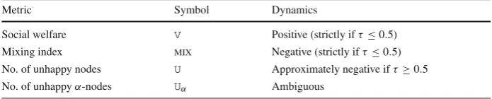
Table 5 Metrics of welfare
Metric Symbol Dynamics
Social welfare V Positive (strictly ifτ≤0.5) Mixing index mix Negative (strictly ifτ≤0.5) No. of unhappy nodes U Approximately negative ifτ≥0.5 No. of unhappyα-nodes Uα Ambiguous
The mixing index of complete segregation (in nontrivial cases) isw(w+1). Sinceρ≤1/2, this means that (with high probability) the process can reach complete segregation only after (nρ−(w+1))/4>nρ/5 stages, i.e.Ω(n)stages. On the other hand, a case analysis shows that ifτ ≤0.5, each step in the process decreases the mixing index by at least 4. This happens because each time a swap occurs, the mixing index decreases by at least 4 (so its not possible that a constant number of nodes swap more thanontimes). We have shown that the second clause of Corollary1(concerning the time to the final state) follows from the first clause.
As another measure of mixing, we may consider the numberkβof maximalβ-blocks in the state. These are the contiguousβ-blocks that are maximal, in the sense that they cannot be extended to a larger contiguousβ-block. LetUbe the number of unhappy nodes in a state. It is not hard to show that ifτ >0.5 thenmix=Θ(U)=Θ(kβ)and in particular
mix≤w·(w+1)·kβ ≤w·(w+1)·U<mix·2w/(1−τ). (1)
This means that the number of unhappy nodes at a certain state reflects the progress of the process towards segregation. More precisely, the metricsmix,kβ,Uare mutually proportional whenτ >0.5, where the analogy coefficient depends onw(see Fig.5). In Table5we display these global metrics of welfare, along with their dynamics. A function (on the stages of the process) has positive dynamics if it is non-decreasing and approximately positive dynamics if it isΘ(g)for some nondecreasing functiong, where the multiplicative constant does not depend onn. Similar definitions apply for ‘negative’. The first clause of Theorem1(the case whenτ >0.5) is the hardest to prove. It turns out that in this case we can deduce a non-trivial lower bound on the mixing index of dormant states.
Lemma 1 (Mixing in dormant states)Consider the process(n, w, τ, ρ)withτ >0.5. The mixing index in a dormant state is more than n(w+1)τρ∗, as long asw >1/(2τ−1).
The caseτ >0.5 is further divided in two cases, which reflect the proportions of happy nodes in the initial state. We display these in Table3, along with the corresponding expecta-tions for the numbers of happy nodes of each type. Lemma1is crucial for the proof of the first clause of Theorem1(in particular the caseτ+ρ <1).
2.2 Accessibility of Dormant States and Complete Segregation
2.2.1 Overview of the Proof of Theorem1for>0.5 and+>1
This argument consists of two parts. First, we show that in this case with high probability the initial state is such that every state with the same number ofα-nodes has unhappy nodes of both types (i.e. it is not dormant). Hence under these conditions, no accessible state is dormant. The second part consists of showing that from every state there is a sequence of transitions to either a dormant state or complete segregation. Moreover the latter fact holds in general, for any values ofτ, ρ, so it can be reused for the case whenτ+ρ <1, in Sect.3. This latter case is more challenging, as it can be seen that there are permutations of the initial state which are dormant.
Lemma 2 (Existence of unhappy nodes)Suppose thatτ > 0.5andρ∗ < τ Then for0 wn, every state of the process(n, w, τ, ρ)has unhappyβ-nodes. If in additionτ+ρ∗>1, every state also has unhappyα-nodes.
Givenρ, by the law of large numbers with high probability (tending to 1, asntends to infinity)ρ∗will be arbitrarily close toρ. Hence we may deduce the absence of dormant states (with high probability) in the case thatτ+ρ >1.
Corollary 2 (Absence of dormant states whenτ >0.5 andτ+ρ >1)Ifρ≤0.5< τand τ+ρ >1then with high probability none of the accessible states of the process(n, w, τ, ρ) is dormant.
It remains to show the accessibility of either a dormant state or complete segregation, from any state of the process. An inductive argument can be used in order to prove this fact, which along with Corollary2shows Theorem1forτ >0.5 andτ+ρ >1.
Lemma 3 (Complete segregation or dormant state)Given0 w n, from any state of the process(n, w, τ, ρ)there exists a series of transitions to complete segregation or to a dormant state.
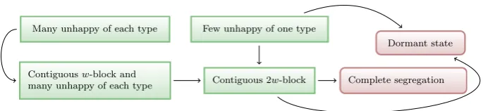
Here is a sketch of the proof. Ifτ≤0.5 the mixing index is strictly decreasing through the transitions, so it is immediate that the process will reach a dormant state (indeed, 0 is a lower bound for the mixing index). For the case whereτ >0.5 (which we assume for the duration of this discussion) we can argue inductively, in four steps. First we show that from a stage with few unhappy nodes of one type (here 5w4is a convenient upper bound of what we mean by ‘few’, which is by no means optimal) there is a series of transitions which lead to either a state with a contiguous block of length 2wor a dormant state. Second, from a state with a contiguous block of length≥2wthere is a series of transitions to complete segregation or to a dormant state. Third, from any state which has at leastw4unhappy nodes of each type, there is a series of transitions to a state with a contiguous block of length at leastw. Finally from a state that has a contiguous block of length≥wand at least 4wunhappy nodes of opposite type from the block, there is a series of transitions to a state with a contiguous block of length≥2w. The combination of these four statements constitutes a strategy for arriving to a dormant state or a state of complete segregation, from any given state. We illustrate this strategy in Fig.8, where two arrows leaving a node indicate that at least one of these routes are possible.
2.2.2 Proof of Lemma2and Corollary2
Contiguous 2w-block
Dormant state
Complete segregation Few unhappy of one type
Many unhappy of each type
Contiguousw-block and many unhappy of each type
Fig. 8 The path to a dormant state or complete segregation whenτ >0.5, proved in Sect.2.2.3
show that ifτ+ρ > 1 then with high probability we may assert that no dormant state is accessible from the initial state.11The following lemma implies Lemma2.
Lemma 4 (Existence of unhappy nodes)Supposeγ ∈ {α, β}and letθ∗be the proportion of γ-nodes in a state of the process(n, w, τ, ρ). Ifτ >0.5andθ∗< τ, then for0wn there exist unhappyγ-nodes in the state.
Proof Given the parametersθ∗, τ,wwhich is large, and any state of the process(n, w, τ, ρ) with no unhappyγ-nodes, it suffices to produce an upper bound onn(which does not depend on the particular state but only onθ∗, τ, wand the fact that noγ-nodes are unhappy). Let δ∈ {α, β} − {γ}. Sinceτ >0.5 and allγ-nodes are happy, there are noδ-blocks of length ≥ w. We may assume thatn > 3w+1. Define thebiasB(I) of an interval I of nodes to be the difference between the number ofγ-nodes in the interval and the number ofδ -nodes in the interval. Without loss of generality suppose that the node occupying sitewis a γ-node (otherwise consider a rotation). We define a sequence(ui)ofγ-nodes in the state,
starting withu0 =w. LetNi denote the neighbourhood ofui. Givenui, defineui+1to be the rightmostγ-node inNi. Since there are noδ-blocks of length≥w, the sequence(ui)
is well defined and it never happens thatui =ui+1. Letm be the largest number such that none of the neighbourhoodsNifor 0<i ≤mcontain the node at site 0. Sincen>3w+1
we havem >0. Let Im= ∪im=0Ni andVm =
m
i=0B(Ni). Note thatImcontains all of the
nodes except at mostw. Moreover sinceui+1−ui ≤wwe have
|Im| ≤2w+1+mw. (2)
LetLi, andRi be the leftmost and rightmostw-many nodes inNi respectively. SinceNi
contains at leastτ(2w+1)nodes of typeγ:
B(Ni)≥(2w+1)(2τ−1) and Vm ≥(m+1)(2w+1)(2τ−1). (3)
Note, however, that some nodes have been counted multiple times in the sum that defines Vm, since the intervalsNi are not disjoint. For eachk∈NletJkmconsist of the nodes inIm
which belong to exactlykdistinct intervalsNi.
By the definition of(ui), the nodeui+2is always outsideNi(since it is aγ-node, and if
it was inNi thenui+1would not be the rightmostγ-node inNi). Similarly,ui+4is always
11On the other hand, ifτ+ρ < 1 then with high probability there are permutations of the initial state
[image:16.439.49.392.52.131.2]outsideNi+2. This means that it is not possible for the neighbourhoods of 5 consecutive terms of(ui)to have a nonempty intersection.12This, in turn, implies thatJkm= ∅for eachk>4.
A similar consideration shows thatJ4mconsists entirely ofδ-nodes (henceB(J4m)≤0). Next, note thatJ1m ⊆L0∪Rm, so|J1m| ≤2w. Hence by counting the multiplicities of the nodes
in the sum which definesVm, we have
Vm=2B(Im)−B(J1m)+B(J3m)+2B(J4m) and Vm≤2B(Im)+2w+B(J3m). (4)
LetNi= Ni−1∩Ni+1and note that Ni= Ri−1∩Li+1. Moreover let Li = Ni∩Li and
Ri = Ni∩Ri. By the definition of(ui)it follows that if Ri is nonempty, then it consists
entirely ofδ-nodes. Sinceui ∈ J3m for eachi ∈ [1,m−1],Ni = Li ∪ Ri∪ {ui}and
J3m⊆ i∈[1,m−1]Ni, we have:
B(J3m) <m+
m−1
i=1
(|Li| − |Ri|). (5)
Letdi =ui−ui−1. Then|Ri| =w−di and|Lk| =w−di+1. Hence|Li| = |Ri+1|and
m−1
i=1
(|Li| − |Ri|)≤ |Lm−1| − |R1| ≤w.
Then from (5) we getB(J3m) <m+w. From the second clause of (3) and (4) we have
2B(Im) > (m+1)(2w+1)(2τ −1)−3w−m. (6)
Ifxm,ym are the numbers ofγ andδnodes inImrespectively, thenxm+ym = |Im|and
xm−ym=B(Im). Hence 2xm= |Im|+B(Im). By hypothesis we havexm ≤nθ∗. Moreover,
sincen≤ |Im| +wwe havexm≤(|Im| +w)θ∗. HenceB(Im)≤(2θ∗−1)|Im| +2wθ∗, so by (2),
B(Im)≤mw(2θ∗−1)+2w(3θ∗−1)+2θ∗−1.
By (6) we may deduce that
2m· [2w(τ−θ∗)−(1−τ)]< w(12θ∗−4τ+1)+4θ∗−2τ−1. (7)
We may assume thatw is larger than(1−τ)/[2(τ −θ∗)]. By this condition and the fact thatτ −θ∗ > 0, the left side of (7) is positive. Also,n ≤ |Im| +w, so by (2) we have
n≤3w+1+mw. If we combine the latter inequality with (7) we get
n<3w+1+w·w(12θ∗−4τ+1)+4θ∗−2τ−1 4w(τ−θ∗)−2(1−τ)
which is the required bound onn.
Note that in the above result, the lower bound that is required onwdepends only onτ, ρ∗, while the lower bound that is required onndepends on τ, ρ∗andw. We may now apply Lemma 4in order to establish the conditional existence of unhappy nodes of both types.
Corollary 3 (Existence of unhappy nodes)Suppose thatτ >0.5andρ∗ < τ. Then if0 wn, every state of the process(n, w, τ, ρ)has unhappyβ-nodes, and ifτ+ρ∗>1then every state also has unhappyα-nodes.
12Sinceu
i+2is outsideNi, the distance betweenuiandui+2is more thanw, and the same holds forui+2
Givenρ, by the law of large numbers with high probability (tending to 1, asntends to infinity)ρ∗will be arbitrarily close toρ. Hence we may deduce the absence of dormant states (with high probability) in the case thatτ+ρ >1.
Corollary 4 (Absence of dormant states)Ifρ ≤ 0.5 < τ andτ +ρ > 1then with high probability none of the accessible states of the process(n, w, τ, ρ)is dormant.
This corollary along with the remark made in Footnote 11 establishes the main dichotomy in the analysis of the process.
2.2.3 Proof of Lemma3(Accessibility of Complete Segregation or Dormant State)
A central part of our analysis is the fact that from any state there is a transition to either a dormant state or complete segregation. This is what we prove in this section. This also means that the only absorbing states of the process are the dormant states.
Ifτ ≤0.5 then it is clear that the only absorbing states of the process are the dormant states, since unhappy pairs of nodes of different type can always swap. Consider themixing indexwhich is non-negative and strictly decreasing in stages forτ ≤0.5. This means that there can only be finitely many swaps in the process, and so a dormant state must eventually be reached.
For the case whereτ >0.5 more effort is required. We argue in four steps. The numbers in what follows are fairly arbitrary. First we show that from a state with at most a small number of unhappy nodes of one type (here 5w4is a convenient upper bound of what we mean by ‘small’, which is by no means optimal) there is a series of transitions which lead to either a state with a contiguous block of length 2wor a dormant state. Second, from a state with a contiguous block of length≥2wthere is a series of transitions to complete segregation or to a dormant state. Third, any state which has at least 2w4 unhappy nodes of each type, there is a series of transitions to a state with a contiguous block of length at leastw, and at leastw4unhappy nodes of each type. Finally from a state that has a contiguous block of length≥wand at least 4wunhappy nodes of opposite type from the block, there is a series of transitions to a state with a contiguous block of length≥2w. The combination of these four statements constitutes a strategy for arriving at a dormant state or a state of complete segregation, from any given state. In the following arguments we will often make use of the following two rather simple facts that hold whenτ >0.5. One is that (ifw > (1−τ)/(2τ−1)), anyβ-node that is adjacent to a happyα-node is unhappy. The second concerns the situation where next to a happyα-node there is aβ-node, and we swap theβ-node for anotherα-node. Then, provided that before the swap the the secondαnode is outside the neighbourhood of theβ-node, both α-nodes will be happy after the swap.
Lemma 5 (Shortage of unhappy nodes)Suppose thatτ >0.5and0wn. From a state with less than5w4unhappy nodes of one of the types, there is a series of transitions to either a dormant state or to a state containing a contiguous block of length at least2w.
Proof Without loss of generality suppose that the state has less than 5w4unhappyα-nodes. Sinceρ∗ ∈ (0,1), and 0 w n, if there does not already exist a contiguous block of length 2wthen there exists an interval[u, v]of 2wnodes which contains at least oneα-node and such that any unhappyα-node is at distance at least 2w2from any node in[u, v].13Any
13Otherwise, everyα-node would be less than 2w2+2w+2 many nodes away from some unhappyα
-node. But there are at least(1−ρ∗)·nmanyα-nodes, and by the previous observation there are at least
unhappyαnode which cannot see any node in[u, v]can move to any position in[u, v]that is adjacent to anα-node (because by doing so, it becomes happy and because if a swap is legal for one member of a potential swapping pair then it is legal for both). Hence we can start successively replacing theβ-nodes in[u, v]which are adjacent toα-nodes, with unhappy α-nodes, each time choosing unhappyα-nodes that have maximal distance fromu, v. Note that this recursive procedure is valid because allα-nodes in[u, v]are happy after each swap. Ultimately we either run out of unhappyα-nodes, or else[u, v]becomes anα-block.
Lemma 6 (Toward a block of lengthw)Supposeτ >0.5. If0wn then from any state which has at least2w4unhappy nodes of each type, there is a series of transitions to a state with anα-block orβ-block of length at leastw, and at leastw4many unhappy nodes of each type.
Proof Suppose that we are given a certain state of the process. Define a sequenceui,i≤w2
ofα-nodes with neighbourhoods Nui respectively, by induction as follows. Letu0 be the
leastα-node whose neighbourhood contains the minimum number ofα-nodes amongst all neighbourhoods ofα-nodes. If ui is defined and i < w2, define ui+1 to be the leastα -node whose neighbourhood is disjoint from∪j≤iNui and whose neighbourhood contains
the minimum number ofα-nodes amongst allα-nodes with the same property (i.e. with neighbourhoods that are disjoint from∪j≤iNui). This completes the definition of(ui), which
is sound provided thatnis sufficiently large. We define a sequencevi,i ≤w2 ofβ-nodes
with neighbourhoodsNvi respectively, in a way entirely analogous to the above definition, ensuring also that all neighbourhoodsNui andNvj are disjoint.
The sequences(ui)and(vi)provide a pool of nodes which will be used for legitimate
swaps in a series of transitions which will lead to the desired state of the process. We start by considering an intervalJ of nodes of length 3wwhich is disjoint from∪j≤w2Nui and
disjoint from∪j≤w2Nvi. Such an interval exists, provided thatnis sufficiently large. LetI
consist of thew-many nodes inJ that are at distance at leastw+1 from any node outside the interval. Clearly any swap that occurs between a node inIand one of the nodesui, does
not affect the composition of the neighbourhoodsNuj for j =i, orNvj for j ≤w2(and
similarly for a swap between a node inIand one of thevi).
Letti,i< wbe the nodes ofIenumerated from left to right. We shall describe a swapping
process, involving less thanw2swaps. At the end of this process of legal swaps, all nodes inI will be of the same type, (but which type that is will not be determined until the end of the process). This process hasw-manysteps, with each stepsinvolving up tosswaps. Let γsbe the type oftsat the end of stages. Also, letVscontain the nodesui, vi,i ≤w2which
are of typeγsand have not been involved in a swap by the end of stages. The construction
is designed so thatγsis the type of allti,i≤sst the end of stages. This feature guarantees
that at the end of the process, all nodes inIhave the same type. Stage 0 is null (i.e. we carry out no instructions at stage 0).
At stages+1 we check ifts+1 has typeγs. If so, then we go to the next stage. If not,
then suppose first thatts+1is unhappy. In the case that ts is happy, any unhappyγs-node
outsideJ can swap withts+1(because an unhappyγs-node moving next to a happyγs-node
cannot decrease its utility). In the case thatts is unhappy, we claim that any nodex from
Vs can legitimately swap withts+1. In order to see this, note that the number ofγs-nodes in
the neighbourhood ofts is at least as large as this number at the beginning of the process.
By the definition ofVs, this number is at least as large as the number ofγs nodes in the
The last case in the procedure is ifts+1is happy and of type different thanγs. In this case
we defineγs+1 ∈ {α, β} − {γs}and swap allti,i ≤swith distinct nodes inVs+1, starting withtsand moving to the left. These are legitimate swaps, as nodes of typeγs+1move next to happy nodes of the same type (so their utility is not decreased after the swap). This concludes the description of the process.
By the end of stagew−1, all nodes inI are of the same type. Since we perform less thanw2many swaps, there are less than 2(2w+1)w2many nodes whose neighbourhoods are affected by these swaps. Sincewis large, there are therefore at leastw4many unhappy
nodes remaining of each type remaining.
Lemma 7 (Toward a contiguous block of length 2w)Suppose thatτ >0.5and0wn. From a state that has anα-block of length≥wand at leastw4unhappy nodes of each type, there is a series of transitions to a state with anα-block of length≥2w. The same holds for β-blocks.
Proof Consider the given state and assume that there is noα-block of length≥2w(otherwise 0 transitions suffice). Let[x,y]be the longestα-block in the given state, and letJconsist of all the nodes that are at distance at leastwfrom the interval[y−2w,y]. Note thatx−1 is a β-node and sinceτ >0.5 it is unhappy. Letzbe the rightmostα-node to the left ofx. Ifzis unhappy, then we may swap it withx−1 since its utility will not decrease. Otherwise, ifzis happy, then it is at a distance at mostwfromxand we may successively swap theβ-nodes in (z,x), starting fromz+1 and moving to the right, for an equal number of unhappyα-nodes inJ. This is possible because each time that we move anαnode next to a happyα-node, the newαnode becomes happy. We repeat this process until anα-block of length 2whas been formed. Each step of the process increases the length of theα-block that is adjacent and to the left ofythe process will terminate. We also perform at mostw many swaps, meaning that we shall not run out of unhappy nodes to perform the swaps with.
Lemma 8 (Complete segregation or dormant state from long block)Supposeτ > 0.5and that0w n. From a state with a contiguous block of length≥2wthere is a series of transitions to complete segregation or to a dormant state.
Proof Consider any state which is not completely segregated, but which has a contiguous block of length at least 2w. Without loss of generality, suppose that this is a block ofαnodes occupying the interval[u, v], where this interval is chosen to be of maximum possible length. Our aim is to show that from this state, one may legally reach another with a contiguous block of greater length (or else a dormant state). Now if the nodesuandvare both happy then the length of the interval ensures that all nodes in the block are happy.14In this case, if there exists an unhappyαnodeu, then lett ∈ {u, v}be distance at leastw+1 fromu. Thenu and theβneighbour oftmay legally be swapped, increasing the length of the run by at least 1.
So suppose instead that at least one of the nodesuandvis not happy, and without loss of generality suppose thatuhasbiasless than or equal tov, where the bias of a node is the number ofα-nodes minus the number ofβ-nodes in its neighbourhood. Thenuandv+1 may legally be swapped. Performing this swap causes positionv+1 to have at least the same bias asvdid before the swap, and causesu+1 to have at most the same bias asudid before the swap. Thus, the swap has the effect of shifting the run one position to the right and may
14Indeed, the neighborhood of any node in(u, v−w]consists of the neighborhood ofu, with some nodes
![Fig. 1 Threshold behaviour when τ, ρ are in [0, 0.5]. The two-dimensional axes refer to τ and ρ](https://thumb-us.123doks.com/thumbv2/123dok_us/1900801.148137/6.439.46.393.297.348/fig-threshold-behaviour-t-r-dimensional-axes-refer.webp)