Reduced invariants from cuspidal maps

White Rose Research Online URL for this paper:

http://eprints.whiterose.ac.uk/152249/

Version: Submitted Version

Article:

Battistella, L., Carocci, F. and Manolache, C. (Submitted: 2018) Reduced invariants from

cuspidal maps. arXiv. (Submitted)

© 2018 The Author(s). For reuse permissions, please contact the Author(s).

[email protected] https://eprints.whiterose.ac.uk/ Reuse

Items deposited in White Rose Research Online are protected by copyright, with all rights reserved unless indicated otherwise. They may be downloaded and/or printed for private study, or other acts as permitted by national copyright laws. The publisher or other rights holders may allow further reproduction and re-use of the full text version. This is indicated by the licence information on the White Rose Research Online record for the item.

Takedown

If you consider content in White Rose Research Online to be in breach of UK law, please notify us by

arXiv:1801.07739v1 [math.AG] 23 Jan 2018

L.BATTISTELLA, F.CAROCCI, C.MANOLACHE

Abstract. We consider genus 1 enumerative invariants arising from the Smyth–Viscardi moduli space of stable maps from curves with nodes and cusps. We prove that these invariants are equal to the Vakil–Zinger reduced invariants for the quintic threefold, providing a modular interpretation of the latter.

Contents

1. Introduction 1

2. M1(Pr, d)- Components, equations and alternate compactifications 6 3. The moduli space of1-stable maps withp-fields 17

4. The weighted 1-stabilisation morphism 26

5. Local equations and desingularisation 40

6. Splitting the cone and proof of the Main Theorem 42

References 50

1. Introduction

While genus 0 Gromov–Witten theory is understood fairly well, the higher genus theory is still unknown in general and its enumerative meaning is affected by more degenerate contributions. The Vakil–Zinger reduced Gromov–Witten invariants solve two problems at the same time: they give computations of genus 1 Gromov–Witten invariants and they have a better enumerative meaning. The only unsatisfactory feature in Zinger’s approach is that the modular interpretation is unclear. In this paper we propose a way to fix this issue by working with a different moduli space.

1.1. Reduced invariants. We briefly recall the definition and the main re-sults which concern reduced Gromov-Witten invariants. The locus of maps from smooth elliptic curves toPr _{is irreducible; we call its closure themain component} of M1,n(Pr, d). In [VZ08] R. Vakil and A. Zinger construct a desingularisation

Date: January 25, 2018.

f

M1,n(Pr, d)mainof the main component via an iterated blow-up construction. Let

e

C f˜ //

˜ π

Pr

f

M1,n(Pr, d)main

be the universal curve over Mf1,n(Pr, d)main and let l ∈ N. Then, the sheaf ˜

π∗f˜∗OPr(l) is a vector bundle. Given X_l a hypersurface of degree lin Pr, Vakil–

Zinger define genus1 reduced invariants ofXl as:

ctop(˜π∗f˜∗(OPr(l)))∩[Mf_1,n(Pr, d)main].

Standard and reduced invariants are related by the Li–Zinger formula [LZ07]:

(1) N1(X5, d) =N1red(X5, d) + 1

12N0(X5, d).

1.2. Cuspidal Gromov–Witten invariants. Based on D.I. Smyth’s work on the birational geometry of M1,n [Smy11a, Smy11b], M. Viscardi [Vis12] has

in-troduced a series ofalternate compactifications of the moduli space of maps from smooth elliptic curves. The first instance of these alternate compactifications is

M(1)_1,n(X, β), where elliptic tails are made unstable and cuspidal singularities are allowed in the source curve. These spaces carry perfect obstruction theories and lead to invariants; we call them cuspidal Gromov–Witten invariants. We conjec-ture the following analogue of the Li–Zinger formula for cuspidal invariants.

Conjecture 1. Let X be a smooth projective threefold, γi ∈ A∗(X). Reduced

invariants with insertionsγi are equal to cuspidal invariants with insertionsγi.

The main result of this paper is that Conjecture 1 holds for the quintic three-fold. More precisely, we have the following.

Main Theorem. Let X5⊆P4 be a generic smooth quintic threefold. Then:

N₁red(X5, d) =N1cusp(X5, d),

where:

N₁red(X5, d) := deg

ctop(˜π∗f˜∗(OP4(5)))∩[Mf₁(P4, d)main]

and

N₁cusp(X5, d) := deg[M (1)

1.3. The proof of the main Theorem. The moduli spaceM1(Pr, d)has many boundary components. From the proof of the Li–Zinger formula we see that the genus0contribution to the right hand side of (1) comes from the boundary com-ponent with a single rational tail. This suggests that discarding this comcom-ponent would provide a more direct approach to reduced invariants for the quintic three-fold. This is exactly what the Viscardi space M(1)₁ (Pr_{, d)} does.

Here is a rough sketch of the proof of our result. We first show:

Theorem. There exists a well-defined 1-stabilisation morphism at the level of weighted-stable curves:

Mwt_1,n,st→Mwt_1,n,st(1)

replacing elliptic tails of weight 0 with cusps.

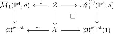
We then consider the following cartesian diagram:

ZX5 M

(1) 1 (X5, d)

Mwt₁ Mwt₁ (1).

We prove that ZX5 is a substack of M1(X5, d) that has no component with contracted elliptic tails. The diagram above endows ZX5 with a virtual class which, by Costello’s virtual push-forward formula [Cos06], has the same enumer-ative content as[M(1)₁ (X5, d)]vir.

In order to compare the degree of[ZX5]vir with Vakil-Zinger’s reduced invari-ants we follow in Chang and Li’s footsteps. We first introduce the moduli space of 1-stable maps with p-fields; this has the advantage of having a simpler ge-ometry and admits a cosection-localised virtual class with the same degree as [M(1)₁ (X5, d)]vir, see [CL12]. We then construct

Mwt₁ ,st×_Mwt,st

1 (1)M (1)

1 (P4, d)p,

and perform a desingularisation of it via the study of local equations [HL10]. In the end we analyse a splitting of the intrinsic normal cone [CL15]. All these steps deliver the theorem.

1.4. Smoothability. On our way there, we review Vakil’s characterisation of maps lying in the boundary ofM1(Pr, d)mainand we give a new proof using Hu-Li’s equations. We also review and extend Smyth’s work on genus1singularities, and rephrase smoothability as follows.

Theorem. A map [f]∈M1(Pr, d) contracting the minimal genus 1 subcurve is

1.5. Relation to other works. We view our result as an analogue of the Li– Zinger formula for cuspidal invariants. The Li–Zinger formula was first proved by J. Li and A. Zinger [LZ07] in the symplectic category and with algebraic-geometric methods by H.-L. Chang and J. Li [CL15]. Our approach is an adaptation of [CL15].

Zinger has computed reduced invariants in [Zin09]. It would be interesting to see if there is a direct calculation for cuspidal invariants. Zinger’s computation together with the Li–Zinger formula gives a computation of genus 1 Gromov– Witten invariants [Zin08].

The reduced Gromov–Witten invariants are related to the Gopakumar–Vafa invariants, and they coincide for Fano targets. Indeed the Gopakumar–Vafa in-variants are by definition related to Gromov–Witten inin-variants by a recursive for-mula which takes into account degenerate lower genus boundary contributions. These contributions were computed by R. Pandharipande in [Pan99]. We do not have reduced invariants for higher genus, but if we had a modular interpretation of the main component, we could view the Gopakumar–Vafa formula as a higher genus analogue of the Li–Zinger formula.

Recently, D. Ranganathan, K. Santos-Parker, and J. Wise [RSW17] have given a modular interpretation of the main component of the moduli space of stable maps via centrally aligned log structures and a factorisation property.

1.6. Outline of the paper. In §2 we review some classical results about the irreducible components ofM1(Pr, d)and local equations for this moduli stack in a smooth ambient space. We recall Smyth’sm-elliptic singularities and Viscardi’s alternate compactifications of the space of maps. We discuss two different proofs of Vakil’s characterisation of smoothable maps to projective space: one is based on Hu-Li’s local equations; for the other one we give a classification of genus 1 singularities.

In §3 we adapt Chang-Li’s work onp-fields to our case: we introduce the moduli space M(1)₁ (P4_{, d)}p of ₁-stable maps with _p-fields, we endow it with a cosection-localised 0-dimensional virtual class supported on a proper substack (depending on a homogeneous polynomial w_{). We show that its degree coincides with the} genus 1cuspidal invariants of the quintic threefold X5 =V(w) up to a sign.

In §4 we argue in two different ways that there is a morphism of Artin stacks

Mwt_1,n,st→Mwt_1,n,st(1)

extending the identity on smooth elliptic curves and replacing elliptic tails of weight0 by cusps. We then use it to define:

Z :=Mwt_1,n,st×_Mwt,st

1,n (1)M

(1)

1,n(P4, d), Zp :=Mwt, st

1,n ×Mwt_1,n,st(1)M (1)

1,n(P4, d)p.

We show that Z is a closed substack of M1(P4, d). Unfortunately we are not able to compareZp _{directly withM}

In §5 and §6 we study local equations and a desingularisation of Zp_{. With}

these in place, we adjust Chang-Li’s splitting of the intrinsic normal cone to our case. This analysis allows us to prove the main theorem.

1.7. Notations and conventions.

• We work over an algebraically closed field kof characteristic ₀.

• We fix a homogeneous polynomial w_∈k_{[x0, . . . , x4]5 of degree 5such thatX5=}

V(w_)⊆P4 is a generic smooth quintic threefold. We usually drop the subscript and writeX for X5.

• We fix a positive integerddetermining all the homology classesβ =d[ℓ]∈A1(P4), line bundle weights, etc.

• M:= Mwt_1,n,st denotes the moduli stack of prestable curves with a weight

assign-ment subject to a stability condition, see §4. The universal curve isπ:C _→M.

• P := Pictotdeg=d_1,n ,st denotes the Picard stack of π:C _{→ M} with universal line

bundleL of total degree _d, subject to the stability condition:

ω_πlog⊗L⊗2 _isπ-ample.

• Mdiv₁ denotes the moduli space of nodal curves with a relative Cartier divisor

satisfying a stability condition, see §2.

• M :=M1,n(X, β) denotes Kontsevich’s moduli space of n-pointed genus 1stable maps to X in the homology class β; we always denote by (π, f) : C_{M → M×X}

the universal curve and stable map.

• Similarly we denote by cM:= Mwt=d_1,n ,st(1) the stack of weighted-stable, at worst cuspidal curves (see §4), with universal curve ˆπ:Cb_→Mc.

• Let Pb denote the Picard stack of πˆ:Cb_→ c_M, with universal line bundle Lcof

total degreedand satisfying the usual stability condition.

• Let Mdiv₁ (1) be the moduli stack parametrising at worst cuspidal curves with a relative Cartier divisor subject to the usual stability condition.

• M :=b M(1)₁ (X, β) is the Smyth-Viscardi’s moduli space of 1-stable maps; we always denote by(ˆπ,fˆ) :Cb

b

M→Mb ×X the universal curve and stable map.

• We usually work with unmarked curves, for we are interested in the Gromov-Witten theory of a Calabi-Yau threefold, son= 0.

• We always denote the spectrum of a discrete valuation ring (DVR) by ∆, with closed point0 and generic pointη.

• Subcurves are always connected. The minimal arithmetic genus 1 subcurve is called thecore or the circuit.

Acknowledgements. This work was inspired by a discussion with Prof. R. Thomas. We thank Prof. T. Coates for useful discussions. L.B. and F.C. would like to thank F. Bernasconi, A. Dotto and Prof. D.I. Smyth for their clever suggestions.

Fellowship. This work was supported by the Engineering and Physical Sciences Research Council grant EP/L015234/1: the EPSRC Centre for Doctoral Training in Geometry and Number Theory at the Interface.

2. M1(Pr, d) - Components, equations and alternate compactifications

2.1. Local equations and components. We start by recalling a description of the global geometry of M1(Pr_{, d). Besides the main component, which was} defined in the Introduction, for every positive integer k and partition λ⊢d into

kpositive parts, there is an irreducibleboundary component Dλ(Pr, d)defined to

be the closure of the locus where:

(i) the source curve is obtained by gluing a smooth elliptic curve E with k

rational tails Ri∼=P1,

(ii) the map contracts the elliptic curveE to a point, (iii) the map has degreeλi on the rational tailRi.

Indeed Dλ(Pr, d) is the image of the gluing morphism from the fiber product:

M1,k× k Y

i=1

M0,1(Pr, λi) !

×₍Pr₎kPr.

We will denote by Dk _{the union of all theD}

λ(Pr, d) where λhas kparts. Proposition 2.1. (1) These are all the irreducible components of M1(Pr, d):

M1(Pr, d) =M1(Pr, d)main∪ [

λ

Dλ(Pr, d).

(2)A map [f] lies in the boundary of the main component if and only if: • either f is non-constant on at least one irreducible component of the core, • or if f contracts the core, write C = E p⊔q Fki=1Ri, where E is the

maximal contracted genus 1 subcurve, then {df(TqiRi)}

k

i=1 are linearly dependent in T_f(E)Pr_.

In this case we say that [f] is smoothable.

This is due to R. Vakil and A. Zinger, see [Vak00, Lemma 5.9][VZ07]. We shall later discuss a proof of this fact based on local equations for the moduli space.

We now review Hu-Li’s procedure for finding local equations ofM1(Pr, d) in a smooth ambient space [HL10]. They will be useful when describing the structure of the intrinsic normal cone and its splitting.

Recall that a map C → Pr _{is given by a line bundle L on C together with}

r+ 1sections inH0_{(C, L)that generate the line bundle. It is therefore natural to} embedM1(Pr, d) as an open inside π∗L⊕r+1 on the universal Picard stack P.

namely that ωπ ⊗OC(2D) is a π-ample line bundle, where D is the universal Cartier divisor. We can construct Mdiv_1,n as the open inside

C(π∗L) = Spec_PSym•(R1π∗L∨⊗ωπ)

(see [CL12] and Section 3 below), where the section of L _{is not 0 on any}

ir-reducible component of the curve. Alternatively this is the moduli functor of a prestable curve with a line bundle and a section up to scalar, which can be thought of as the hom-stack HomM1(C,[A1/Gm]); then we should pick the con-nected component where the line bundle has total degreed, and the open substack obtained by requiring weighted stability and the section not to vanish on any ir-reducible component of the curve. The morphism Mdiv_1,n → P is obtained by declaringL

Mdiv_1,n :=OC(D).

Let[f:C→Pr_{]be a point ofM1(}Pr_{, d): we may fix homogeneous coordinates} onPr in such a way that_D:=f−1_{{x0 = 0}} is a simple divisor supported on the smooth locus ofC, i.e. a d-uple of distinct smooth points; this property will then hold in a neighbourhood of [f]. This gives a morphism from an étale chart U

of M1(Pr, d) to an étale chart V of Mdiv1 . We may assume that V is contained in the locus where the divisor consists of d distinct smooth points; notice that such locus is smooth overM1. A map to Pr shall now be thought of as a curve-divisor pair(C, D)together with rsections of O_{C(D); the map can be written as}

[1 :u1 :. . .:ur], where 1denotes the given section ofOC →OC(D).

Furthermore, étale locally on M1(Pr_{, d), we may pick extra sectionsAand B} of the universal curve C _→M1(Pr_{, d)} such that:

(1) they pass through the core;

(2) they are distinct smooth points disjoint from the support of D.

Nowπ∗OC(D+A) is a vector bundle on V and π∗OC(D) is carved inside it by the vanishing of the restriction mapπ∗OC(D+A)→π∗OC(D+A)|_A.

Proposition 2.2. (1) There is a locally closed embedding of an étale chart of M1(Pr, d) inside the vector bundle V := Spec_V(π∗OC(D+A)⊕r):

M1(Pr_{, d) U V}

Mdiv₁ V

´ et

´ et

Notice that V is smooth sinceV is.

(2)Assume furthermore that V is affine; onV we then have:

π∗OC(D+A)∼=π∗OC(D+A−B)⊕π∗OC(D+A)|B

and restricting to Ais zero on the second factor.

(3)Call ϕ:π∗OC(D+A−B)→π∗OC(D+A)_|A the map induced on the first

sum of line bundles: let D=Pd_i=1δi, then

ϕ=⊕ϕi: ⊕id=1π∗OC(δi+A−B)→π∗OC(D+A)_|A.

After choosing a trivialisation for each of the line bundles above, ϕi: OV → OV is given by multiplication by

Y

q∈[A,δi]

ζq,

where ζq is the smoothing coordinate on M1 corresponding to the node q, and [A, δi]denotes the set of nodes separating A (the core) from the point δi.

We may now choose coordinates (wj_i)j_i,...,d=1,...,r on the fiber of V → V compat-ible with the basis given in Proposition 2.2 .(3) such that U is an open inside

F1 _{=. . .=F}r_{= 0 ⊆V, where:}

Fj = d X

i=1   Y

q∈[A,δi]

ζq  wj_i.

We refer the reader to [HL10, Lemma 4.10, Proposition 4.13] for the details; we are going to review the key ideas in §5, where we find local equations forM(1)₁ (Pr_{, d)}.

We include here a proof of Proposition 2.1 .(2) based on Hu-Li’s equations.

Proof. Let us start with the easiest degenerate situation: a contracted elliptic curve attached to a P1 of degree_d at a single node_q. Equations for the moduli space of maps around such a point look like:

ζq d X

i=1

w_ij = 0, for j= 1, . . . , r.

Our point corresponds to a smoothable map if and only if the equations admit a solution with ζq 6= 0, that isPd_i=1wj_i = 0 for every j. Taking a coordinate z

on P1 _{centred at the node q, the i-th basis vector corresponds to a polynomial} vanishing at q and at δl, ∀l6=i. This can be written as:

ei(z) =z Y

l6=i

(z−δl)

−δl

,

where we have chosen a convenient normalisation. So the restriction to the ratio-nal tail of the map corresponding to the point of coordinates (wj_i)j_i=1=1_,...,d,...,r can be written as:

[1 : d X

i=1

w_i1ei(z) :. . .: d X

i=1

Differentiating with respect toz we see that the image of the tangent vector atq

is given in affine coordinates around f(E) by:

( d X

i=1

w1_i, . . . ,

d X

i=1

w_ir).

Hence smoothability is equivalent to the image of the tangent vector being zero. More generally we may assume that the dual graph is terminally weighted [HL10, §3.1]. Assume there arekrational tails of positive weightRh, h= 1, . . . , k.

Denote byD(h) the set of indicesisuch that δi belongs to theRh, and byE(h)

the set of nodes separating the core from Rh. The equations will then take the

following form: k X h=1   Y

q∈E(h)

ζq  

  X

i∈D(h)

wj_i



= 0, j= 1, . . . , r,

which can be assembled in matrix form as follows:

W ·ζ :=   X

i∈D(h)

wj_i

  j,h ·   Y

q∈E(h)

ζq  

h = 0.

We see that smoothability is equivalent to the linear dependence of the rows of the above matrixW. On the other hand we can choose a suitable coordinate zh

around the nodeqh on Rh and write the map as: [1 :p1_h(zh) :. . .:prh(zh)],

where:

pj_h(zh) = X

i∈D(h)

w_ijeh_i(zh) and ehi(zh) =zh Y

l∈D(h)\{i}

(zh−δl)

−δl

.

The elliptic curve is contracted to the point[1 : 0 :. . .: 0]and the tangent vector toRh atqh is mapped to theh-th row ofW (in affine coordinates aroundf(E)).

Again we see that the map is smoothable if and only if the image of the tangent vectors to the rational tails at the nodes are linearly dependent in T_f(E)Pr. 2.2. Smyth-Viscardi’s compactifications. The moduli spaces ofm-stable maps give alternate compactifications ofM1,n(X, β), parametrising maps from smooth

elliptic curves.

Definition 2.3. Let C be a connected, reduced, projective curve of arithmetic genus1over k, and let_{p1, . . . , pn∈C}be smooth, distinct points. A map_{f:C →}

X is said to be m-stable if the following conditions hold:

(1) C has only nodes and elliptic l-fold points, l≤m, as singularities. (2) For any subcurveE ⊂C of arithmetic genus 1 on whichf is constant,

(3) f has no non-trivial infinitesimal automorphisms.

Recall that a k-rational _p∈C is called an_{elliptic m-fold point} if:

ˆ

O_C,p∼₌

    

k_{[[x, y]]/(y}2_−x3_{) m= 1} k_{[[x, y]]/(x(x−y}2_{)) m= 2} k_{[[x, y]]/Im m≥3}

where Im = (xhxi−xhxj :i, j, h∈ {1, . . . , m−1}) andi, j, h are distinct.

Viscardi’s main result [Vis12, Theorem 3.6] is the following:

Theorem 2.4. The moduli functor of m-stable maps M(₁m_,n)(X, β) is represented by a proper Deligne-Mumford stack of finite type over k_.

Remark 2.5. The Behrend-Fantechi obstruction theory R•πˆ∗fˆ∗TX for spaces

of morphisms endows M(₁m_,n)(X, β) with a perfect obstruction theory relative to

M1,n(m). The base is an irreducible Artin stack for every m and even a smooth

stack for m ≤ 4. We thus have a virtual class on M(₁m_,n)(X, β) and m-stable invariants can be defined in the usual way.

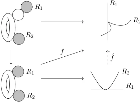
Remark 2.6. We think that the algorithm proposed by Viscardi to prove the properness of his moduli spaces oversees a case. The issue is that, given a map

f: C_{∆ →} Pr

∆ over a DVR scheme ∆ such that Cη is smooth and f0 is constant on a genus 1 connected subcurve E ⊆C_{0, it is not always true that f descends}

to a map_fˆ_:Cb_∆→Pr

∆, where Cb0 has a genus 1Gorenstein singularity. Consider the stable map [f]inM1(P3,4) from an elliptic bridge

C:=R1q1⊔E⊔q2 R2

to P3 that maps _R1 to the _z-axis, contracts _E to the origin, and makes _{(R2, q2)} into the normalisation of a cusp in the (x, y)-plane, i.e. its image is the non-Gorenstein singularity:

D:= Spec (k_{[x, y, z]/(x, y))∪Spec} k_{[x, y, z]/(z, y}2_−x3_). Notice thatdf(Tq2R2) = 0, so there is a non-trivial linear relation:

0·df(Tq1R1) + 1·df(Tq2R2) = 0,

and hence the map is smoothable. Viscardi claims that the map factors through the familyCb_{∆, obtained by contractingE to a tacnode. Notice that the image of}

ˆ

f would still beD, since there is at most one indeterminacy point ofCb_∆99KPr ∆, located at the singularity. However in our example f cannot factor through the tacnode. Indeed in that case we would have a birational morphism between two singular curves with the same δ invariant and the same normalisation, so

ˆ

f:Cb→ Dwould be an isomorphism, which is a contradiction. We suggest that in this case the correct procedure would be to sprout(R1, q1).

However Viscardi’s argument can be fixed. Let (C_{η, Fη) be a stable map to}

R1

R2

R1

R2

R1

R2

R1

R2

f

ˆ

f

Figure 1. An example of non-factorisation.

smooth [Vis12, Section 3.2.1]. As described in [Vis12, Theorem 3.6, Step 1], after applying nodal reduction we get a mapF:C_∆′ →Pr

∆′, for which we may suppose

thatC :=C_{0 is nodal and reduced, andf :=F0 is stable.}

If f is not constant on the minimal genus 1 subcurve, then it is already m -stable and there is nothing to say. Otherwise let E⊂C be the maximal genus1 subcurve wheref is constant and letR1⊔. . .⊔Rm=C/E.

By Proposition 2.1 (2) we know there is a non-trivial linear relation among thedf(TqiRi)’s. Consider a maximal one with all non-zero coefficients. Possibly

after relabelling, such a relation looks like:

α1df(Tq1R1) +. . .+αjdf(TqjRj) = 0.

In this case we blow-up C_{∆ in qj+1, . . . , qm. The induced map F}˜_{0 is constant}

on the exceptional divisors Gj+1, . . . , Gm and we can complete the above linear

relation to

α1d ˜f(Tq1R˜1)+. . .+αjd ˜f(TqjR˜j)+βj+1d ˜f(Tqj+1Gj+1)+. . .+βmd ˜f(TqmGm) = 0

withβi = 1 for all i. Now this sprouting [Smy11b, Section 2.3] ensures that the

map descends to the corresponding elliptic m-fold singularity. Notice that, for every m1 ≤ m2, there is a morphism from an m2-elliptic singularity to an m1 -elliptic point that is birational on the target and contracts m2−m1 branches of the source to the singular point. Proceed now with Step 2 of Viscardi’s algorithm.

The irreducible components of Viscardi’s moduli space M(₁m_,n)(Pr_{, d) are also} well understood [Vis12, Thm. 5.9]; indeed they have a similar description to the ones of Kontsevich’s space. The main advantage of them-stable compactification is that the number of components drops asm increases.

2.3. Genus 1 singularities and smoothability. Inspired by Viscardi’s alter-nate compactification, we give another description of smoothable maps in genus 1.We recall the following:

Definition 2.7. Let C be a reduced curve over k _{and p ∈ C a singular point.} We define thegenus of the singularity inp to be the quantity:

g(p) =δ(p)−b(p) + 1,

where δ(p) = dimk(ν∗O_C/OC)⊗k(p), ν:C →C is the normalisation of C at p,

andb(p) is the number of branches ofC at p.

Proposition 2.8. Let [f:C → Pr_{] be a stable map from a genus 1 curve C =}

Ep⊔qFm_i=1Ri, where E is the maximal genus1 subcurve contracted byf, and the

Ri are rational tails on which f has positive degree.

Then f is smoothable if and only if it factors through a curve with a genus 1

singularityf:C−→φ Cb −→fˆ Pr_{, such thatφcontractsExc(f) and is an isomorphism}

outside it.

Lemma 2.9. (Classification of genus 1 singularities) The Cohen-Macaulay (i.e. reduced) genus 1 singularities with m branches are obtained by gluing a genus 0

singularity with k branches together with a Smyth’s (m−k)-elliptic fold. Notice that k may be 0 (i.e. a point) or1 (i.e. a smooth rational curve).

Proof. We extend the argument given by Smyth [Smy11a, Appendix A] to classify the Goreinstein genus 1 singularities. We study the analytic germ of the singu-larity and we adopt Smyth’s notation: R denotes the completion of the local ring of C at the singularity; Re = k_{[[t1]]⊕. . .⊕}k_[[tm]] its integral closure; _mR the maximal ideal of R andm_Re that ofR.e

Let us recall that to describeR as a quotient polynomial ring, it is enough to find a k-basis for _mR/m2

R = he1, . . . , esik where the ei are some elements in R.e

Indeed, once given such a basis, it is a consequence of completeness thatRcan be recognised ask_{[[x1, . . . , xs]]/I}, where_I is the kernel of the ring homomorphism

k_{[[x1, . . . , xs]]→R⊂}k_{[[t1]]⊕. . .⊕}k_[[tm]]

xi 7→ ei

Smyth observes thatR/Re is graded by:

(R/Re )i:=mi_Re/(mi_Re∩R) +mi_Re+1

Furthermore:

(1) m=δ(p) =P_i≥0dimk(R/Re )i;

(2) 1 =g(p) =P_i≥1dimk(R/Re )i;

From (2) and (3) it follows thatdimk(R/Re )1= 1 anddimk(R/Re )i = 0for i≥2.

Then the exact sequence:

0→ m

2

e

R

m2_e

R∩R

→ mRe

m_Re∩R →(R/Re )1 →0

entails that:

m2_e

R⊆mR, mR/m 2

e

R⊆mRe/m2Re is a codimension 1k-subspace.

Obviously m2_R ⊆ m2_e

R. Hence s is at least m −1. After relabelling we may

assumee1, . . . , em−1 generate mR/m2_Re, and after Gaussian elimination they take

the following form:

e1 = (t1,0, . . . ,0, a1tm)

e2 = (0, t2, . . . ,0, a2tm)

. . .

em−1 = (0,0, . . . , tm−1, am−1tm)

witha1, . . . , am−1 ∈k. At this point Smyth restricts his attention to Gorenstein singularities and shows that under this assumption he can choose all the ai to

be 1. Furthermore m2_e

R =m 2

R holds if m ≥3, thus the above are generators for

mR/m2R and the goal is reached. For m = 1 (resp. 2) he finds extra generators

and shows they satisfy the equation of a cusp (resp. a tacnode).

Removing the Gorenstein restriction we have three possibilities for m≥3: (1) At least two of theai are non-zero, say i= 1,2: thena1a2t2m=e1·e2 so

m2_e

R = m 2

R and we are done as above. It is easily seen that e1, . . . , em−1 satisfy the equations of a(k, m−k)singularity where kis the number of

ai that are zero.

(2) Only one of the ai is non-zero, saya1= 1: then m_R2_e=m2R+ (t2m)and by

adjoining em =t2m to the ei we see that they generate mR/m2_R and they

satisfy the equation of a tacnode(e2

1−em)em = 0, and eiej = 0 for i6=j

and (i, j) 6= (1, m), so this is an (m−2,2) singularity.

(3) Finally all theaiare zero: then we have to addt2m, t3mto generatemR/m2R

and we find an (m−1,1) singularity.

Similarly for m = 2 there are two possibilities: the tacnode (corresponding to

a1 6= 0) and the union of a cusp with a non-coplanar line (for a1 = 0), with equations:

k_{[[x, y, z]]/(xz, yz, y}2_−x3_).

Form= 1the only possible singularity is the cusp: indeed it can be proven that

m2_e

R=mR.

invariant that distinguishes them is:

dimkR/Ip

where

Ip = AnnR(R/Re ) = n

f ∈ R|f·Re⊆Ro

is the conductor ideal at the singular point. Using the explicit description of R

given in the lemma above, we can easily find generators of Ip and check that for

a(k, m−k) singularity we have:

dimkR/Ip=m−k. Lemma 2.11. Every genus 1 singularity is smoothable.

Proof. We explicitly construct a (semi)stable model with a contraction to the given singularity. Assume we start with a (k, m−k)-singularity Cb. Pick any

m-pointed elliptic curve (E, q1, . . . , qm) and glue E along the markings with m

copies of P1 at their respective points ₀; call the rational tails _{R1, . . . , Rm}. It is useful to consider the resulting curve C as a point of M1,2m with markings

on the rational tails given by 1 and ∞. We now choose a smoothing C_∆ of _C

over a DVR scheme∆, such that the total spaceC_{∆has anA1-singularity at the}

nodesq1, . . . , qk and is regular everywhere else; furthermore extend the markings

to get a horizontal Cartier divisor Σ. Resolving the singularities we obtain a fibered surfaceπss:Css

∆ →∆ such that in the central fiber the strict transforms e

R1, . . . ,Rek are at distance 1 from the core E, while the other rational tails are

adjacent to it. Call F1, . . . , Fk the exceptional divisors of the resolution. As in

[Smy11a, Lemma 2.12] we may contractE, which is obviously balanced, by means of the line bundle:

L_{1 :=ωπ}ss(E+ Σ),

which results inC_{∆with anm-elliptic singularity in the central fiber,kof whose}

branches are the images of F1, . . . , Fk and are thus unmarked. We may finally

perform a second contraction by using the line bundle L_{2 :=} O

C_∆(Σ); let Cb∆ denote the resulting family of curves, with singularity qˆ. Notice that L₂ satisfies

cohomology and base-change, hence we may simply check on the central fiber both its relative semi-ampleness and the behaviour of its sections. The sections will be constant along F1, . . . , Fk, so the linear relation among their derivatives

at the Smyth’s singularity will only imply the linear dependence of the tangent vectors ofRbk+1, . . . ,Rbm at qˆ; on the other hand sections ofL2 alongR1, . . . , Rk

are completely independent, and thus they embed these P1. We deduce that the central fiber of Cb_{∆has a (k, m−k)-singularity.}

Proof. 2.8 The argument that if f is smoothable then it has to factor through a genus 1 singularity was essentially given by Vakil in [Vak00, Lemma 5.9]. We review it here in some detail.

trivial on every irreducible component of the central fiber contracted byf. Since every connected component of Exc(L_{) ={D ⊂C :}L_{|D ≃}O_{D} has arithmetic}

genus 0 or 1, we may use the argument in [Smy11a, Lemma 2.12] to show that

L _{is π∆-semi-ample. We thus get a contraction φ:}C_∆→C_{∆ and notice thatF}

factors through φby the construction of C_{∆= Proj}

∆ L

n≥0π∆,∗L⊗n

. Being a smoothing of a reduced curve, C_{∆ is normal, thus φ factors through the}

nor-malisation ν:Cb_{∆ →} C_{∆, which is a finite map by [Liu02, §8.2]. It is now clear}

thatCb_{∆→∆is a flat family of genus1 curves with reduced fibers, and the map} F◦ν has positive degree on all the components of Cb_0.

Viceversa let us suppose that we have a factorisation:

C Pr

b

C

f φ fˆ

such that φ contracts Exc(f) and is an isomorphism everywhere else. We shall below make the point that f is smoothable as soon as it is not constant on the core (compare also with [RSW17, Theorem 4.5.1]), so in this case we have no use forφ. Otherwiseφcontracts at least the core, andCb has a genus1singularity at a certain pointq. We first show that:

Claim 1. Under these assumptions, we can produce smoothings C_{∆ ofC and}Cb_∆

of Cb with a contraction map φ∆ extending the given φ.

A statement of this kind is in general far from true, see Remark 2.12 below. The proof of this claim follows the lines of the two-step contraction described in the proof of Lemma 2.11. It will be useful to treat C as a stable curve marked withf−1(Q) for a generic quadric Q⊆Pr_.

Proof. Assume thatCb has a(k, m−k)-singularity atq; denote byE :=φ−1(q)⊂

C, which is the maximal genus 1 unmarked (i.e. contracted by f) connected subcurve of C. By assumption the components of C adjacent to E are marked (i.e. not contracted by f), and they can be partitioned intoR1, . . . , Rk mapping

to the genus0part of the(k, m−k)-singularity, andRk+1, . . . , Rmparametrising

the branches of the (m−k)-elliptic fold. Let li denote the distance of Ri from

the core Z, which can be determined from the marked dual graph. Let l = max{lk+1, . . . , lm}andL= max{l1, . . . , lm}. Consider a smoothingC∆ofC with an Al−li singularity at Ri ∩E for i =k+ 1, . . . , m, and an AL−li+1-singularity

at Ri∩E for i= 1, . . . , k. Extend the markings f−1(Q) to a horizontal Cartier

divisorΣ. LetCss

∆ be the semistable model with regular total space; notice that in the central fiber the strict transforms of Rk+1, . . . , Rm are at distance l from

the core, while all other marked components are further apart. Let Ebal _{be the} maximal unmarked balanced subcurve inside Css

at distance less thanl fromZ. We may now use Smyth’s line bundle:

L_{1 =ωC}ss ∆/∆

  X

F⊆Ebal

(l+ 1−l(F, Z))F



⊗O_Css ∆(Σ),

to perform the contraction of Ebal, obtaining a family C_{∆ → ∆} whose central

fiber has an m-elliptic fold point. Notice that the contraction is otherwise an isomorphism, due to the stability condition. As in Lemma 2.11 we may then perform a second contraction by using the line bundleL_{2 :=}O_C

∆(Σ); we denote by Cb_{∆the resulting family of curves. It may be seen that the central fiber} Cb_{0 is}

isomorphic to Cb, and so is the resulting contraction up to an automorphism of

C.

LetLc_{be an extension of L}b_{:= ˆf}∗O_Pr(1)onCb, which exists because deforming

line bundles on curves is unobstructed. In order to extend fˆto Fb:Cb_∆→Pr all we have to show is that the r+ 1 sections ˆs0, . . . ,ˆsr+1 representing the map fˆ extend to sections of Lc_.Thus it is enough to verify that_H1_(C,b _Lb_{) = 0} [Wan12].

Once this is done we are going to obtain the smoothing of the original map by precomposing with the contraction F:C_∆−→φ Cb_∆−F_→b Pr_.

Since all the curves we are considering are Cohen-Maculay, they have a dual-ising sheafω_Cb such that for any line bundle Lb:

H1(C,b Lb) = (H0(C,b Lb−1⊗ω_Cb))∨.

It is known [Ser00, IV, § 3] that ω_Cb can be described as the subsheaf of ν∗ω_C⊗

K(C) (whereν: ¯C →Cbis the normalisation) satisfying: for every openU ⊆Cba rational1-formω ∈ν∗ ω_C⊗K(C)(U)is a section of ω_Cb(U) if and only if:

X

q∈ν−1₍₀₎

Res(ν∗(f)ω) = 0 ∀f ∈O b

C(U)

From this description it is patent that the pullback ofω_Cb to the normalisation restricts to a line bundle of degree−1or0 on every branch, according to it being one of thek or m−kcomponents. Hence it can be seen from the normalisation exact sequence and Serre duality that H1(C,b Lb) = 0 as soon as Lˆ has positive

degree on one of the branches.

Remark 2.12. In general it is not possible to find compatible smoothings as above: pick any genus 2 curve with a rational tail and map it to the ramphoid cusp, a planar singularity with local equation y2−x5 = 0. Then a compatible smoothing can be found only if the rational tail is attached to a Weierstrass point of the genus 2 curve, as can be seen by computing the semi-stable model of the ramphoid cusp. This example was kindly suggested to us by Prof. D.I. Smyth.

depends on its restriction to thek rational tails, namely it is independent of the

k-pointed elliptic curve thatf contracts.

3. The moduli space of 1-stable maps with p-fields

We adapt Chang-Li’s theory of p-fields to cuspidal maps. This is a word-by-word repetition of the arguments in [CL12] once noticed that they carry over to families of at worst cuspidal curves. We provide the non-expert reader with a résumé of some of the key ideas contained in [CL12]; this section can otherwise be skipped.

3.1. Moduli of sections.

Definition 3.1. LetB be an algebraic stack and let π:C _→B be a flat proper

morphism of finite presentation, which is representable by algebraic spaces, and whose geometric fibers are reduced l.c.i. curves. Let Z be an algebraic stack,

representable, quasi-projective, and smooth over C_{. The cone of sections of} Z

over C is a _B-stack_Sdefined by:

S(S →B) ={sections ofZ_{S →}C_S};

The groupoid Sis an algebraic stack representable and quasi-projective over

B [CL15, Proposition 2.3].

To fix the notation let us draw the following diagram:

Z

C_S C

S B

e

πS π

where e denotes the universal section. Let us see some examples of the above

construction we will be interested in.

Direct image cones. WhenZ _{= Vb(}L₎ for a line bundle L on C, the algebraic

stack S→B representing sections ofL _{can be constructed as:} C(π∗L) := Spec_BSym•(R1π∗L∨⊗ωπ).

This is essentially because R1π∗L∨⊗ωπ commutes with pullbacks, and it has

the desired modular interpretation by Serre duality.

Moduli of stable maps and 1-stable maps. Recall that P denotes the universal

Picard stack. Let X ⊆Pr _{be a projective variety and let} Z_{X be defined by the}

Z_{X X×}C_P

L⊕r+1_\0C Pr_×C_P

/G_m

/G_m

Then M1(X, β) is the open substack of the moduli space SX of sections of

Z_{X →} C_{P defined by the stability condition. This is the point of view we have}

already taken for X = Pn in Proposition 2.2 to describe the local equations of the moduli space of maps.

Analogously the moduli space of1-stable maps M(1)₁ (X, β) can be thought of as an open inside the moduli space of sections of

c

Z_{X = (Vb(}Lc⊕r+1 b

P )\0Cb)×PrX

over Cb b

P.

Moduli of1-stable maps with p-fields. In this section we denote by Mb the moduli space of1-stable mapsM(1)₁ (P4_{, d)} and byPc

b

M=Lc ⊗−5

b

M ⊗ωˆπMb.

The moduli space ofp-fields is defined as the cone of sections of the line bundle c

P b

M over CbMb:

Definition 3.2. The moduli space of1-stable maps withp-fields:

M(1)₁ (P4_{, d)}p _:=C(ˆπ

b

M,∗(PcMb)) parametrises 1-stable maps:

b

C_S P4

S

ˆ fS

ˆ πS

with ap-fieldψˆ∈H0(Cb_S,fˆ∗

SOP4(−5)⊗ω_ˆπS).

We use the abbreviation Pb :=M(1)₁ (P4_{, d)}p. Employing the above description of the moduli space of1-stable maps,Pb can also be thought of as an open in the moduli space of sections of the vector bundle Vb(Lc⊕5

b

P ⊕PcPb).

3.2. Obstruction theories. With the above, the morphism S → B admits a relative dual perfect obstruction theory:

φ_S/B:T_{S/B →}E_{S/B := R}•_πS,∗e∗_TZ/C

For the proof see [CL12, Proposition 2.5] and notice that it relies on general properties of obstruction theories and the cotangent complex, and the fact that

Z _→C is smooth, but never on the specification thatC _→Bis a family of_nodal

curves.

• for the direct image cone of a line bundle L _{the dual obstruction theory}

is E_{C(π∗L)/B = R}•_π∗L_;

• the moduli space M =b M(1)₁ (P4_{, d)} has a dual obstruction theory relative to Pb given by E

b

M/Pb = R •_πˆ

b

M,∗( L4

0LcMb);

• in the case of 1-stable maps with p-fields Pb = M(1)₁ (P4_{, d)}p, we get E_b

P/Pb = R •_πˆ

b

P,∗(Lc ⊕5

b

P ⊕PcPb).

We review the compatibility of various obstruction theories for the moduli spaces mentioned above.

Lemma 3.3. Pb is a smooth Artin stack of dimension 0. Furthermore there is a compatible triple of dual perfect obstruction theories:

ˆ

ρ∗T

b

P/Mb[−1] TMb/Pb TMb/Mb

R•πˆ_Mb,∗(O b

C) R

•_πˆ

b

M,∗( L4

0LcMb) R

•_πˆ

b

M,∗(fM∗bTP4)

≀

[1]

[1]

implying that E_b

M/Pb = R •_πˆ

b

M,∗( L4

0LMb) gives the standard Behrend-Fantechi-Viscardi virtual class onMb.

Proof. The first statement follows from deformation theory: the projectionρˆ:Pb →

c

M is unobstructed of relative dimension 0 and cM is a smooth Artin stack of di-mension 0, since both nodal and cuspidal singularities are l.c.i., so obstructions to their deformations are contained in Ext2O_b

C(ΩCb,

O b

C) = 0.

The fact thatT

b

M/Mb →EMb/Mb := R •_πˆ

b

M,∗(fM∗bTP4)is a perfect obstruction theory

when Cb_{→ M}b is a family of Gorenstein curves is proved in [BF97, Proposition

6.3].

The lower row in the above diagram is induced by the Euler sequence of P4. The middle column comes from identifying the space of stable maps as an open substack of the cone of sections (see above) of Vb(L4₀Lc_{)over P}b_{. The existence}

of such a commutative diagram is [CL12, Lemma 2.8]. The final claim follows

from functoriality of virtual pullbacks [Man12].

Lemma 3.4. There is a compatible triple of dual perfect obstruction theories

(R•πˆ_Pb,∗(Pc_b

P),R

•_πˆ

b

P,∗(Lc ⊕5

b

P ⊕PcPb),R

•_πˆ

b

P,∗(Lc ⊕5

b

P )) for the triangle:

b

P Mb

b

P

Notice that the virtual rank of E_b

P/Pb := R •_ˆπ

b

P,∗(Lc ⊕5

b

P ⊕PcPb) is 0, hence it endows the moduli space of 1-stable maps with p-fields with a cycle class of di-mension0. However Pb is not proper. In the next section we describe Chang-Li’s cosection (depending on the choice ofw_∈k_{[x0, . . . , x4]5}) of the obstruction bun-dle, and show that the corresponding localised cycle is supported on the proper subtackM(1)₁ (X, d),where X=V(w₎is the quintic threefold, that is the degen-eracy locus of the cosection.

3.3. Cosection localisation and virtual pullback. Recall Kiem-Li’s machin-ery of cosection localised virtual classes [KL13, Theorem 1.1]:

Theorem (Localisation by cosection). Let Y → S be a morphism of DM type between algebraic stacks, withY Deligne-Mumford andS smooth, endowed with a perfect obstruction theory. Suppose the obstruction sheafObY admits a surjective

homomorphism σ: ObY|U→OU over an open U ⊆Y.

Let ι:Y(σ) :=Y \U ֒→Y, then(Y, σ) has a localised virtual cycle:

[Y]vir_loc∈A∗Y(σ).

This cycle enjoys the usual properties of the virtual cycles; it relates to the usual virtual cycle [Y]vir _via[Y]vir _=ι

∗[Y]vir_loc∈A∗Y.

We now review a slight generalisation of this, that combines it with Manolache’s virtual pullback construction [Man12]; this can also be found in [CL12, § 5].

LetY →Sbe as in the hypotheses of the theorem, or more generally such that there is a triple of compatible obstruction theories for a triangleY →S→T with

T smooth. Assume for simplicity that the obstruction theory E_{Y /S is a vector} bundleE admitting a cosection:

E−→σ O_Y

surjective on an openU ⊆Y; denote by Y(σ) the complement Y \U. Recall the following notation from [KL13]:

G= Ker (E|U →OY|U), E(σ) =E|Y(σ)∪G. Kiem and Li define a localised Gysin map:

s!_σ,loc:A∗(E(σ))→A∗(Y(σ)),

which we explain in what follows. Let [B] ∈ Z∗(E(σ)) be a cycle represented by a closed integral substack. If B ⊂ E|Y(σ) then they use the standard Gysin morphism:

s!_σ,loc[B] :=s!_E|

Y(σ)[B]∈A∗(Y(σ)).

Suppose instead thatB is not contained inE|_Y(σ).Then we may choose a variety with aregularising morphism Ye −→ν Y such that:

• the pullback along ν of the cosection ν∗_{σ =: ˜σ extends to a surjective} morphism

ν∗E−→σ˜ O e

Y(D)→0

for a Cartier divisor D⊆Y .e

• there is a closed integral Be ⊂ Ge = Ker(˜σ) such that ν˜∗[Be] = k[B] for some k∈N_.

We denote byν(σ) : D→Y(σ) the restriction ofν to the divisor, and byν˜:Ge→

E(σ) the restriction of the natural map ν∗_{E →E. The localised Gysin pullback} is then defined as:

s!_σ,loc[B] := 1

kν(σ)∗

[D]·s!_Ge[Be] ∈ A∗(Y(σ)).

In [KL13, § 2] they prove that: such (Y , ν,e Be) always exist; the cycles!_σ,loc[B]is independent of the above choices; the construction preserves rational equivalences and thus defines the desired morphism on Chow groups.

Remark 3.5. If we consider[Y]as a cycle inE(σ), thought of as the zero section ofE, notice that a natural choice for Ye isBl_Y(σ)Y.

Kiem and Li then proceed to extend the cosection-localised Gysin pullback to vector bundle stacks h1/h0(E₎ (this is relatively easy in the presence of a global resolution, which is the case in the situation at hand); they show that the intrinsic normal coneC_{Y /S} is contained in the closed substack h1/h0(E_)(σ),at least when the cosection of the relative obstruction bundle lifts to a cosection of the absolute obstruction bundle [KL13, Corollary 4.5].

Definition 3.6. Consider a cartesian diagram of stacks:

Y′ Y

S′ S

ϕ′ ρ′

ρ

ϕ

withρ as above. Assume furthermore that we have a cosection Ob_Y/S→O_Y

that lifts to a cosection of the absolute obstruction sheaf ObY. Then we can define a localised virtual pullback operation:

(ρ′)!E_Y′_/S′,σ′:A∗(S ′_)→A

∗−rk(E)(Y′(σ′)) where E_Y′

/S′ = (ϕ′)∗E

Y /S, σ′ = (ϕ′)∗(σ) andY′(σ′) =Y(σ)×Y Y′.

Replace S′ _{by a primitive cycle in it, i.e. assume that S}′ _{is irreducible and} reduced. Recall that pulling backE_{Y /S} along_ϕ′ endows_ρ′ with a relative perfect obstruction theory. Furthermore we can pullback the cosection:

ObY′_/S′ ∼=ϕ∗Ob_Y/S σ′

The degeneracy locus of σ′ _{is Y}′_(σ′_{),which in turn implies that:}

h1/h0(E_Y′

/S′)(σ′) = (ϕ′)∗h1/h0(E

Y /S)(σ).

By [KL13, Corollary 4.5] and from the cartesian diagram above,

C_Y′

/S′ ⊆(ϕ′)∗C

Y /S ⊆EY′ /S′(σ′)

thus we can define the localised virtual pullback of [S′]to be:

(ρ′)!E_Y′_/S′,σ′[S ′_{] =s}!

σ′_,loc[C_Y′_/S′].

3.4. A cosection for p-fields. We are going to construct the cosection paral-leling [CL12, §§3.2-3.4]. There is a morphism of vector bundles on Pb induced by iterated tensoring of line bundles:

h1: Vb(Lc_Pb⊕5⊕Pc_Pb)→Vb(ωπˆ_Pb), h1(x,p) = pw(x0, . . . ,x4) By differentiating it and pulling it back along the universal evaluation

Vb(Lc⊕5 b

P )\ {0} ⊕Vb(PcPb)

b

C b

P CbPb

b

P Pb

e

ˆ

π_Pb πˆ_Pb

we obtain a cosection of the relative obstruction sheaf

σ1: ObPb/Pb = R 1_ˆπ

b

P,∗(Lc ⊕5

b

P ⊕PcPb)→R1πˆPb,∗(ωπˆPb)≃OPb

σ_1|(u,ψ)(˚x,˚p) = ˚pw_{(u) +ψ}

4 X

i=0

∂iw(u)˚xi

(2)

The degeneracy locus of this cosection isM(1)₁ (X, d): by Serre duality ifw_(u)6=

0 then we can find a p such that the cosection does not vanish; similarly we can do if ψP4_i=0∂iw(u) = 06 . But w(u) = 0 and ∂iw(u) = 0 never happen

simultaneously by smoothness ofX, so it has to bew_{(u) =ψ= 0.}

Moreover Chang and Li prove that σ1 lifts to a cosection of the absolute ob-struction bundleOb_Pb →O

b

P;it has the same degeneracy locus becauseObPb/Pb → Ob_Pb is surjective. This is a sufficient condition for the relative intrinsic normal cone to be contained in the closed substack of the obstruction bundle determined by the cosection, see § 4.4.

We may thus endow M(1)₁ (P4_{, d)}p with a localised virtual cycle: [Pb]vir_loc= 0!_σ1,loc[C_Pb/Pb] ∈ A0

We want to show that it gives the same numerical invariants as the cuspidal Gromov-Witten theory of X, up to a sign:

Theorem 3.7.

deg[M(1)₁ (P4_{, d)}p_]vir

loc= (−1)5ddeg[M (1)

1 (X, d)]vir

3.5. From p-fields to the quintic threefold. This is achieved in two steps: we first compare the invariants ofM(1)₁ (P4_{, d)}p with the ones of_M(1)_{1 (NX/P}4, d)p, where N_X/P4 is the normal bundle of the quintic in P4.

Second we compare the latter invariants with deg[M(1)₁ (X, d)]vir.

Deformation to the normal cone. This is attained in [CL12, §§4-5] by a family version of thep-fields construction applied to the deformation to the normal cone ofX⊆P4; let us denote the latter by_{V →}A1_t, so that_{Vt6=0 =}P4and_V0=NX/P4. Lemma 3.8. The deformation to the normal cone V is cut insideVb(O_P4(5))× A1

t with basis coordinates [x0 : . . . : x4] and fiber coordinate y by the equation

w_{(x)−ty = 0. If C(V) denotes the affine cone over V, then its tangent bundle} is determined by the following exact sequences:

0→T_C(V)/A1

t →O

⊕5

C(V)⊕OC(V)

P

i∂iw(x)˚xi−t˚y

−−−−−−−−−−→O_C(V)→0

(3)

0→T_C(V)→O⊕5

C(V)⊕OC(V)⊕OC(V)

P

i∂iw(x)˚xi−t˚y−y˚t

−−−−−−−−−−−−→O_C(V)→0

(4)

This allows a description of the moduli space of maps to V as the cone of sections of a certain smooth object Z′ _over Cb

b

P×A1:

Z′ _V

Vb(L⊕5 b

P )\ {0} ⊕Vb(L ⊗5

b

P ) Vb(OP4(5))×A 1 t

b

C

M(1)1 (V)

b

C b

P×A1_t

M(1)₁ (V,(d,0)) Pb ×A1_t

e

ˆ π

M(1)₁ (V) πˆPb×_A1

t

Similarly Vb :=M(1)₁ (V,(d,0))p can be defined as the cone of sections ofZ _:= Z′_⊕Vb(Pc

b

P). The general theory explained above provides an obstruction theory

for Vb→Pb ×A1

t [CL12, Proposition 4.2]:

Lemma 3.9. A dual perfect obstruction theory is given by:

φ_Vb/Pb×A1

t:

T_b

V/Pb×A1

t →

E_b

V/Pb×A1

t := R

•_πˆ

b

V(f

∗

b

wheref_Vb:Cb b

V →V is the universal map andH is the vector bundle onV defined by the exact sequence, see (3):

0→H _→pr∗

P4 OP4(1)⊕5⊕OP4(5)

Pi∂iw(x)˚xi−t˚y

−−−−−−−−−−→pr∗P4OP4(5)→0.

The restriction ofφ_Vb/Pb×A1

t to a fiber

b

Vt= (

b

P t6= 0

M(1)₁ (N_X/P4, d)p t= 0

gives the standard obstruction theory of Vbt→Pb.

We would like to conclude that the restriction of the virtual cycle to the fibers is the standard virtual cycle on the fiber. The techniques of functoriality in inter-section theory teach us that we should look for a triple of compatible obstruction theories for the triangle:

b

Vt Vb

b

P

ιt

The cone of sections interpretation provides us with an obstruction theory relative to Vb →Pb given by:

E′

b

V/Pb := R •_πˆ

b

V(f

∗

b

VK ⊕PcVb)

where K is determined by the following exact sequence on _V, see (4):

0→K _→pr∗

P4 OP4(1)⊕5⊕OP4(5)⊕OP4

P

i∂iw(x)˚xi−t˚y−y˚t

−−−−−−−−−−−−→pr∗P4OP4(5)→0

Of course h0(E′

b

V/Pb)≃TVb/Pb, but the previous lemma and the difference between

H _andK _{hint at the fact that the obstruction sheafh}1₍E′

b

V/Pb)contains one factor R1ˆπ_Vb,∗O

b

C_b V ≃

O b

V too many, so that restricting E′Vb/Pb to the fibers we would not

find their standard obstruction theory. A confirmation of this fact is given by observing that E′

b

V/Pb equips Vb with a 0-dimensional cycle, while we are looking

for a 1-dimensional cycle such that restricting to any fiber, i.e. applying ι!_t, we get[Vbt]vir ∈A0(Vbt).

This issue is solved in [CL12, §§4.5-6] by lifting the standard obstruction theory

φ′

b

V/Pb to a different, specifically tailored one:

φ_Vb/Pb:T_b

V/Pb →EVb/Pb,

where the latter two-term complex fits into an exact triangle:

R1πˆ_Vb,∗O b

C_b

V[−2]→ E_b

V/Pb ν

− →E′

b

V/Pb [1]

Furthermore φ_Vb/Pb is compatible with the standard obstruction theory for the fibers:

Lemma 3.10. For every t∈A1

k we have a commutative diagram:

ˆ

π_Vb

c∗ O b C b Vc

[−1] E

b

Vc/Pb

E

b

V/Pb|Vbc

T≤1

b

Vc/Vb

T≤1

b

Vc/Pb

T≤1

b

V/Pb|Vbc

For the proof see [CL15, § 4.6]. Notice that the lower row is not a distinguished triangle, yet Chang and Li prove in [CL12, A.4] that this weaker (truncated) notion of compatibility is enough to prove functoriality.

Since we are working with cosection localised cycles, we need a family version of the cosection. This is induced by differentiating the following vector bundle morphism onPb ×A1_t:

Vb(Lc⊕5 b

P ⊕Lc ⊗5

b

P ⊕PcPb)

(pr2,pr3)

−−−−−→Vb(Lc⊗5 b

P ⊕PcPb) ·

−

→Vb(ωπˆ_Pb) The cosection takes then the following form:

Ob_Vb/Pb×A1 ⊆R1πˆ∗(Lc_Vb⊕5⊕Lc_Vb⊗⊕Pc_Vb)→R1πˆ∗ωπˆ ¯

σ1|(u,v,ψ)(˚x,˚y,p˚) =ψ˚y+v˚p

It is showed in [CL12, §4.7] that σ¯1 lifts to a cosection σ¯: Ob_Vb → O_Vb and that the degeneracy locus ofσ¯ is

M(1)₁ (X, d)×A1_t.

Recall that the sections (u, v) are required to satisfy w_{(u)−tv = 0. So σ¯1} coincides up to a non-zero scalar with the above defined cosectionσ1 for Pb when

t6= 0. It is proved in [KL13, Theorem 5.2] that, given compatible perfect obstruc-tion theories, the construcobstruc-tion of a cosecobstruc-tion localised virtual cycle is compatible with Gysin pullbacks, so that by [CL12, Proposition 4.9]:

ι!_t6=0[Vb]_σ¯vir= [Pb]vir_σ ∈A0(Qb), ι!0[Vb]virσ¯ = [M (1)

1 (NX/P4, d)p]_σvir_¯0 ∈A₀(Qb) where we have denoted by Qb:=M(1)₁ (X, d).

Functoriality of cosection-localised pullback. We prove thatdeg[M(1)₁ (N_X/P4, d)p]vir_σ¯ 0 coincides up to a sign with deg[M(1)₁ (X, d)]vir. In the rest of the section we use the following notation: Nc:=M(1)₁ (N_X/P4, d)p, andvˆ:Nc→Qb.

First, Chang and Li prove that there is a perfect obstruction theory

E

b

N/Qb:= R

•_πˆ

b

N,∗(Lc ⊗5

b

compatible with E

b

N/Pb and ˆv ∗_E

b

Q/Pb, so that ENb/Qb inherits a cosection σ′0 with degeneracy locus D(σ₀′) =Qb. So they have a localised virtual pullback:

ˆ

vE! _b

N/Qb,loc:A∗(Qb)→A∗(D(σ ′

0) =Qb)

which they then prove to satisfy functoriality using the techniques of [KKP03], so:

ˆ

vE!_b

N/Qb,loc[Qb]

vir _{= [M}(1)

1 (NX/P4, d)p]vir_σ′

0.

To conclude it is enough to compute the degree of ˆv!

E_b

N/Qb,loc on A0( b

Q); we just need to compute deg(ˆv!

E_b

N/Qb,loc[ζ]) for a closed point ζ. This is done in [CL12, Theorem 5.7] and the same considerations work in our case.

Hopefully we have managed to convince the reader that the subtle intersection theory perpetuated in [CL12] does not rely at all on the hypothesis that the families of curves we are working with arenodal, butl.c.i. curves are well-behaved enough so that all the proofs carry over to the situation of our interest.

4. The weighted 1-stabilisation morphism Before stating the main result of this section we recall the following:

Definition 4.1. Mwt=d_1,n ,st denotes the stack of weighted-stable curves of genus 1 with n markings and total weight d: geometric points of Mwt=d_1,n ,st represent

connected, reduced, nodal, projective curves of arithmetic genus1withndistinct smooth markings and an integer-valued functionwt on the dual graph.

Such a function assumes only nonnegative values, the sum of which on all the vertices of the dual graph isd;wtis compatible with the specialisation maps, and we further impose the following stability condition:

• every pa= 0 component of weight 0 has at least three special points;

• every pa= 1 component of weight 0 has at least one special point.

There is an étale, non-separated morphism Mwt=d_1,n ,st → M1,n. The stability

condition is such that the forgetful map M1,n(Pr, d) → M1,n factors through

Mwt=d_1,n ,st, the weight coming from the degree of the map toPr.

Definition 4.2. Let Mwt=_1,n d,st(1) be the stack of at worst cuspidal connected, reduced, n-marked, projective curves of arithmetic genus 1 that are weighted-stable with total weightd, i.e. the weight is nonnegative and such that:

• every pa= 0 component of weight 0 has at least three special points;

• every pa= 1 component of weight 0 has at leasttwo special points.

Remark 4.3. It follows from the miniversal deformation of the cusp that being at worst cuspidal (i.e. having only nodes and cusps as singolarity) is an open condition on the base of any family of curves.

Theorem 4.4. There exists a morphism Mwt=_1,n d,st →Mwt=_1,n d,st(1) which extends the identity on the smooth locus.

As anticipated we explain two different approaches to the proof:

(1) we first construct a substack of the productMwt=_1,n d,st×Mwt=_1,n d,st(1)which plays the role of the graph of such a morphism, and then check that the projection onto the first factor is an isomorphism;

(2) we prove that the1-stabilisation exists at the level of curves with a divisor constructing the contraction directly, then argue that it descends to a morphism between moduli spaces of weighted curves.

4.1. First approach: the graph. Recall the shorthand notationM=Mwt=_1,n d,st

and cM=Mwt=_1,n d,st(1), with universal curves π:C _{→M and πˆ:}Cb_→c_M

respec-tively. Abusing notation we will still write C _and Cb_{for their pullbacks to the}

product M×cM along the two projections.

Lemma 4.5. There is a locally closed substack X ⊆ Mor_M×Mb(C_,Cb₎

represent-ing morphisms that contract genus 1 tails of weight 0 to cusps, and are weight-preserving isomorphisms everywhere else.

Proof. Recall thatMor_M×Mb(C_,Cb_{)is an algebraic stack; in fact the map toM×}c_M

is representable by algebraic spaces [Ols06]. Let φ:C _→Cb_{denote the universal}

morphism. We now proceed to construct X as a locally closed substack in the space of morphisms.

Step 1: We first lift the problem to the level of Picard stacks in order to trans-mute the property of being weight-preserving into the more manageable one of preserving the line bundles. Recall the notation:

λ:P=Pictotdeg_1,n =d,st→M, λˆ:Pb =Pictotdeg_1,n =d,st(1)→Mc

for the Picard stacks of π and πˆ respectively, with universal line bundles L

andLc_{. We can now look at the algebraic stack Mor}

P×Pb(C,Cb)with universal

morphism Φ and natural projection Π to Mor_M×Mb(C_,Cb₎. There exists a

lo-cally closed substack Y′ _⊆Mor

P×Pb(C,Cb) representing those morphisms that

preserve the line bundles. Indeed, given a smooth chart S →Mor_P×Pb(C_,Cb₎,

the locus ofs∈S where Φ∗_sLc_s∼₌L_{sis nothing but the locus T where the two}

sections L_{S and Φ}∗