Stochastic analysis of surface roughness : a fractal-based approach

(1)

S to c h a stic A n aly sis o f S u rface R o u g h n e ss

A F ra c ta l-b a s e d A p p ro a c h

Steven John Davies

July 1998

(2)

D e c la ra tio n

Unless otherwise specified in the text, this thesis describes my own work, supervised by Professor P. G. Hall.

.0

(3)

A ck n o w led g em en ts

To my wife, Robyn, for her much needed support and encouragement.

To my parents, John and Jacqueline, who made many sacrifices so that I would receive the best possible education.

To my supervisors and mentors, Peter Hall, Nick Fisher & Graham Constantine. They provided the problem, guided me through my attem pts at tackling it, and carefully scrutinised the end result.

To my friend, Dan Lunn, for his constant badgerings. I hope now that we can change the subject.

(4)

A b s tr a c t

The need to characterise surface roughness arises in many branches of science and en gineering, in areas as diverse as soil science, polymer chemistry and manufacturing. The ability to capture information about surface properties with a few statistical in dicators can provide the basis for control and monitoring of industrial processes, and the indicators themselves may be important covariates in scientific investigations.

In the past, the extent of an analysis of roughness has been limited largely to calculation of some simple roughness parameters. Although these parameters are appealing by virtue of their ease of calculation, they do not perform well in terms of characterising surfaces and, from a statistical point of view, there are many problems

associated with their use.

The two main aims of this thesis are to provide better parameters for characteris ing surface roughness, and to provide statistical tools to aid scientists and engineers in making inferences. In developing the methodology, special care has been taken to make the methods as practicable as possible.

The main parameter chosen to characterise surface roughness is fractal dimen sion. It has the appealing property that, when using it to judge whether one surface is rougher than another, the decision will, in many circumstances, agree with the subjective ordering made by a trained observer. This is a property the parameters in current use do not enjoy.

(5)

dimension, being a scale-invariant measure, does not take account of such a dif ference. So a parameter called topothesy, which is scale-sensitive, is introduced to complement fractal dimension.

Many methods have been proposed for estimating fractal dimension from data, but little attention has been given to understanding how the estimators perform. This thesis includes theoretical and numerical analyses of the performance of esti mators of fractal dimension and topothesy in a number of different situations.

The analyses provide a guide to how well estimators will perform in general, but do not quantify the precision of an estimate calculated from a given data set. So, this thesis also proposes methods to calculate standard errors of fractal dimension and topothesy, thereby providing an objective way of making comparisons between surfaces. Methods for carrying out hypothesis tests are also discussed.

Roughness characterisation methods are also developed for two-dimensional data. In the past, most of the data sets used to gauge surface roughness were one dimensional profiles, collected along a straight path across a surface. As a result of advances in both the technology for measurement equipment and the storage capac ity of computers, genuine two-dimensional surface data sets are now quite common. This raises the important question of anisotropy: how do the roughness proper ties of the surface vary with orientation? This question is thoroughly explored and appropriate methods devised.

(6)

C ontents

A b s tr a c t iv

1 In tr o d u c tio n 1

1.1 M otivation... 2

1.2 Examples of applications... 3

1.3 Visualising the d a ta ... 8

1.4 Statistical m o d e llin g ... 10

2 C h a r a c ter isin g surface ro u g h n ess 15 2.1 Review of existing methods ...17

2.2 What is roughness?... 19

2.3 Fractal m eth o d s... 21

2.3.1 Fractal dimension and fractal in d e x ... 21

2.3.2 Point estimation ... 23

2.3.3 T opothesy... 28

2.4 Comparison of existing and fractal m e t h o d s ...30

3 T h e v ariogram 34 3.1 D e fin itio n ... 36

3.2 E stim ation... 37

3.3 Advantages of variogram over autocovariance...41

3.4 Exploratory a n a ly s is ...42

3.5 P ro p e rtie s... 49

3.5.1 One-dimensional c a s e ...50

(7)

CONTENTS vii

3.5.2 Two-dimensional case...53

4 O n e -d im e n sio n a l tr a n se c ts 57 4.1 Point estimation ... 59

4.1.1 Theoretical performance of estim ators...59

4.1.2 Numerical issues ...61

4.1.3 Choice of k ... 63

4.1.4 Possible im provem ents...64

4.2 Quantifying the e r r o r ... 65

4.2.1 Plug-in m e th o d ...66

4.2.2 Bootstrap method ...67

4.3 Fitting a variogram m o d e l...69

4.3.1 Model v a lid a tio n ...73

4.4 Effects of measurement e rr o r ...78

4.4.1 Effects of smoothing the v a rio g ra m ... 79

4.4.2 Effects of zeroing the smoothed v a rio g ra m ...80

4.5 Analysis of the roller d a t a ...83

5 Iso tr o p ic su rfaces 87 5.1 Extension from one dim ension...88

5.2 Box c o u n tin g ... 96

5.3 Application to soil surfaces... 100

6 A n iso tr o p ic su rfa ces 104 6.1 General a n is o tro p y ... 105

6.2 Weak anisotropy ... I l l 6.3 A test for isotropy ... 113

6.3.1 Comparing fractal dimension between su rfa ce s...115

6.4 Analysis of the polymer surfaces...116

(8)

C hapter 1

Introd u ction

Fractal analysis of surface roughness is more than a mathematical curiosity. It

has many applications in science and engineering, where it is used to aid understand

ing of the physical processes occurring at the interface between objects or between an

object and its environment. In this chapter we describe examples of such applica

tions from three different disciplines. The examples are elaborated throughout the

thesis, providing the motivation for the methods developed and illustrations of how

the methodology can be applied.

As in most areas of statistical practice, visualisation has an important role to

play. We look at conventional ways of visualising surfaces in three dimensions:

contour plots, wireframe perspective plots and height encoded images. These are

arguably good devices for discerning the features of relatively smooth surfaces, but

they lack clarity and intepretability when used to visualise rough surfaces. One

natural way to view such data is to artificially reconstruct its appearance to the

human eye. This is achieved by computer-generated renderings of the surfaces.

A thorough statistical analysis must necessarily be based on assumptions set out

clearly in mathematical terms. We describe the stochastic framework that we shall

use to model the surface data. We also detail other m ajor assumptions made about

the data used throughout the thesis, and provide physical and statistical justification

for them.

(9)

CHAPTER 1. INTRODUCTION 2

1.1 M o tiv a tio n

The scientific interest in surface roughness is extensive, as can be judged from the vast literature on the subject. As well as journals solely devoted to the topic, such as The Journal of Tribology, there are many articles in a variety of fields.

A large portion of the literature is concerned with physical effects of surface roughness, usually in the setting of particular applications. For example, Thomas & Atkinson (1997) consider the ‘Ammonium uptake by coral reef - effects of water velocity and surface roughness on mass transfer’; and Amis (1996) addresses ‘The effect of surface roughness in fibroblast adhesion in vitro’. Some of the many phys ical properties studied are absorption, magnetisation, adhesion, impedance, flow, growth, friction, conductivity, reflectance and heat transfer.

Another portion of the literature concentrates on the effects of processes, both natural and manufactured, on surface roughness. Two recent examples are McCarrol & Nesje (1996), who study the use of ‘Rock surface roughness as an indicator of degree of rock surface weathering’; and Hassan (1997), who studies ‘The effects of ball- and roller-burnishing on the surface roughness and hardness of non-ferrous metals’.

The remainder of the literature is concerned with the measurement and charac terisation of surface roughness. Measurement is usually achieved through contact methods such as stylus profilometry, or non-contact methods using optics or even acoustics (Swart et al., 1996). An overview of the various characterisation methods is given in Chapter 2.

The development of statistical methods for analysing surfaces has typically been driven by the technologies used to record data. A relatively old but still rather common approach to measurement is stylus profilometry, in which a fine stylus is drawn across a surface and the current generated by its oscillations is taken as a measure of height. The total electrical charge resulting from these oscillations is proportional to the mean absolute deviation of surface height, not the mean squared deviation. Therefore, L\ measures of variation can be more attractive than L2

(10)

recent technologies allow extensive and detailed surface height data to be recorded, and so permit more sophisticated, flexible approaches to data analysis. The new advances include refinements to the performance of stylus profilometers, and optical profilometry based, for example, on scanning with a laser, or with white light from an optical fibre.

However, all profilometer data are recorded from what are essentially line tran sects of the surface (albeit with a non-infinitesimal width representing the diameter of the stylus or light beam) and so are still rather restrictive. New technologies such as scanning electron microscopes allow genuinely two-dimensional data to be gath ered, typically in the form of digital images. Such data offer exciting opportunities for addressing issues of anisotropy and spatial variation in a way that is difficult even for extensive profilometer data. This thesis is motivated by these possibilities. We suggest new methods for analysing surface data, taking advantage of the new technologies and allowing questions of spatial variability to be addressed.

1.2 E x a m p les o f a p p lica tio n s

The following examples have motivated much of the work within the thesis and are used throughout to illustrate how the methodology could be applied.

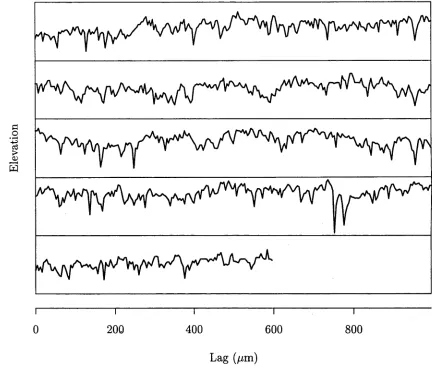
Roller profile In the manufacture of rolled products such as sheet metal and

paper, the surface roughness of the roller is crucial. If the roller is too smooth, it may slip or skid, causing tears in the product. On the other hand, if the roller is too rough this adversely affects the quality of the rolled product, for example by causing perforations. Therefore it is important for the surface roughness of a roller to lie within predetermined control limits. In order to prevent the manufacturing faults mentioned, the rollers are periodically inspected for wear measured in terms of adverse changes to the surface roughness.

(11)

I I I I I

0 200 400 600 800

Lag (/im)

Figure 1.1: The roller profile data broken up into 5 segments with consecutive segments plotted down the page. The scale at the bottom applies both horizontally and vertically.

roller. The stylus had a nominal tip radius of 4/im. The electrical signal giving the profile height, is recorded continuously but is digitised at discrete intervals, approximately 4/rni each, by the instrument used to produce the data.

The data are shown in figure 1.1 and a roughness analysis is performed in Chap ter 4.

Soil surfaces In Soil Science, considerable attention is being placed on under

[image:11.531.53.487.88.458.2]

(12)

(a) 0.00mm (b) 5.30mm (c) 10.05mm

(d) 14.30mm (e) 18.55mm (f) 22.50mm

[image:12.531.13.521.22.683.2]

(g) 27.00mm (h) 31.25mm (i) 35.50mm

Figure 1.2: Rendered images of the soil surface, dry and after eight successive periods of rainfall. The cumulative amount of rainfall is indicated in the caption for each

panel.

(13)

is an important factor in determining the effects of such processes. Contributing to the complexity of the problem is the dynamic nature of the surface as it varies with time due to these and other processes, for example rain and cultivation.

The data we have come from a particular study to assess the availability of water for plant growth after rain. Rainfall itself changes the surface topography through the impact of raindrops and the transportation of particles with the movement of water over the surface. Therefore it is necessary to understand the effect of rainfall on the soil surface as well as the effect of surface topography on the behaviour of water. The water that infiltrates the surface becomes available for plant growth; the remainder either evaporates or runs off. To infiltrate the surface the water needs to be stationary, collected in depressions on the surface, or travelling at low velocity. The surface roughness contributes to the number and size of such depressions and the speed at which water can flow.

A single surface measuring 600mm x 500mm was constructed in the laboratory with dry soil, a sandy loam sampled from Cowra, in South-Eastern Australia. Under the soil was a layer of free-draining coarse sand. The central 512mm x 450mm area of the surface was scanned by a laser device. Height averages over circular regions approximately 0.5mm in diameter were taken at 1mm intervals along parallel lines 1mm apart. The soil surface was then subjected to simulated rainfall consisting of 2.7mm drops falling vertically 13 meters and achieving 97 percent terminal velocity. The rainfall intensity was 90 mm per hour, which would correspond to a heavy storm in the region from which the soil was sampled. Rain was allowed to fall until ponding occurred. (Ponding is the phenomenon of free water appearing on the surface due to rainfall exceeding infiltration.) The surface was then scanned again. The process was repeated 8 times in all, with a night between each rainfall, yielding a time series of 9 images of the soil surface.

The soil surface data are rendered in figure 1.2 and a roughness analysis is given in Chapter 5.

Polym er surfaces The aim in the third application was to identify whether two

(14)

(a) STM 16

.%m v>

[image:14.531.14.520.21.746.2]

y ' X ’Cä:'

• /

|r># ' i if I . *%r (

> - v'^<

Vjf

f a , - * : #

£ i . ^ t K

(b) STM 35

(c) STM 43 (d) STM 52

(e) STM 70 (f) STM 75

Figure 1.3: Rendered images of the six polymer surfaces.

roughness properties.

(15)

wraps offer less opportunity for such organisms to adhere. Another contribution of statistical analysis is to compare surfaces in terms of smoothness.

The data set comprises three pairs of samples of the polymers, one sample from each pair produced by one manufacturing process and the other sample by an alter native process. Both samples in a pair were produced with similar input parameters to the process. The input parameters were different between pairs.

The surface elevations of each polymer sample were measured by coating it with a layer of gold just a few molecules thick, and analysing the coated plastic using a scanning, tunnelling electron microscope. The data from this source were recorded on a 128 x 128 grid, in the form of measurements that were height averages very close to grid point centres. For these data, pixels were 40 nanometres square.

The polymer surfaces data are rendered in panels of figure 1.3 and a roughness analysis is given in Chapter 6.

1.3 V isualising th e data

Visualisation is an important tool in many statistical applications. For the surface scientist, visual characterisation plays an important and sometimes crucial role in topography analysis. Stout et al. (1993, page 197) state that “it is generally ac cepted that a full intuitive appreciation of a surface can only be achieved by 3-D visualisation methods and that 2-D profiles are inadequate for qualitative assess ment.”

Profile data Nevertheless, if the only data available are profiles, then it is still

of value to get an appreciation of the nature of the data by a simple graph. When analysing the surface roughness of profiles using a simple scatterplot of heights against position, features to which one might pay particular attention are the irreg ularity of the sample path and the scale of its oscillations. To do this consistently, equal scalings should be applied to both the heights and the positions.

(16)

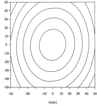
(a) contour plot (b) perspective plot

(d) rendered image (c) height encoded image

Figure 1.4: Four different visualisations of the first polymer surface data

sequence of points. The original surface probably followed a far more irregular path between successive points.

Gridded data There are several common ways of viewing the 3-D surfaces in 2 di

[image:16.531.11.519.18.676.2]

(17)

graphs end up a mess of ink in which it is hard to discern features.

One relatively recent way of viewing raw surface height data is to construct an image of the surface similar to how it would appear to the human eye. The eye remains the most powerful and versatile processor, particularly when complicated and ill-defined but patterned data are involved. A “rendered” image is created by calculating how much light from a particular source would be reflected to the viewer in a particular location. Figure 1.4 is a comparison between a contour plot, a perspective plot, an image plot and a computer rendered scene of the surface. Notice, in panel (d), that we can see evidence of directional dependence in the texture, something which may not be seen in the other graphs except by a trained observer.

The sequence of rendered images for the soil surfaces is shown in Figure 1.2. With careful inspection, it is possible to see how the surface is changing over time with successive amounts of rainfall. The higher areas are gradually being eroded, whereas deposits are being formed in the lower areas. This is easier to see if the individual ‘snapshots’ are animated to form a short movie sequence and played in time, allowing the viewer to switch between scenes both backwards and forwards.

Figure 1.3 shows the surfaces of the six plastic sheets. The fourth sample appears smoother and more regular than the others, although its fractal analysis was not markedly atypical; in fact its fractal properties are on a much finer scale than the

“bubbles” .

1.4 Statistical modelling

(18)

on the real plane for surface data. Therefore the data from a single surface/profile, £(•), is really one datum from an underlying random field X(-).

Since it is hard to carry out any statistical analysis from a single datum, we need to make some assumptions concerning the properties of these processes in order to obtain an effective increase in the sample size. In doing so, we should also ensure that any assumptions made are reasonable, both statistically and physically. By ‘reasonable’ we mean that they need not necessarily be true, but that they are close enough to the truth that any departure will have a negligible effect on the assumption-based methods.

The first assumption we make is that of intrinsic stationarity, which is defined for a random field (process) through first differences:

E[ X( s + t ) - X { s ) } = 0,

var [Ar (s + t) — X(s)] = v(t).

That is, the random field has constant expectation, and the variance of the difference of the random field at two locations depends solely on the relative displacement between the two locations and not on their positions. The function v{t) is known as the variogram and is studied in detail in chapter 3.

An earlier form of intrinsic stationarity is the intrinsic hypothesis of Matheron (1971). The intrinsic hypothesis differed in that it allowed for a linear drift in the process X(-).

The first part of the assumption, namely, that the random field has constant expectation, is not as unreasonable as might first appear considering the nature of the data. In the case of the practical examples outlined in section 1.2, the data are often taken on a much finer scale than the whole surface, so any change in the trend over the whole surface would be slight over the range of the data. The second part of the assumption requires that the process that produced the surface, again at the scale on which the data were collected, behaves in a uniform manner.

(19)

data, where the soil surfaces were artificially constructed, but not for the polymer data, where the polymer is manufactured by an extrusion process: the polymer is drawn out in one direction. More formally, this assumption is that of isotropy and is a tightening of the intrinsic stationarity assumption where we now require that the variance of the difference of the random field at two locations depend solely on the distance, rather than displacement, between the two locations, and not on their relative orientation:

var [X(s + t)- Ar(s)] = u(||t||).

The function v(||£||) is now one-dimensional, as it would be if the random field were itself one-dimensional. Accordingly we call the distance ||t|| the lag, to follow one-dimensional time series terminology. Methods for characterising surface rough ness from two-dimensional data assuming isotropy, and from one-dimensional profile data, are considered and applied to the soil surface data in Chapter 5.

If a random field is not isotropic then we say it is anisotropic. Methods for deducing whether a surface is either isotropic or anisotropic, and methods for char

acterising the surface roughness for anisotropic surfaces, are given and applied to the polymer data in Chapter 6.

When deriving performance properties, it is sometimes necessary to assume that the surfaces may be modelled by Gaussian processes. Indeed, Thomas (1982, page 9) writes:

Many formative processes, particularly those carried out in controlled conditions in research laboratories, can produce textures with height distributions that are accurately Gaussian. Their Gaussian nature is not an artifact: it arises as the natural result of a well-known statistical property, and will occur whenever a texture is created as the cumulative result of a large number of randomly located events.

(20)

In order to compare the asymptotic properties of one-dimensional and two- dimensional estimators, the properties will be expressed in terms of overall sample size, iV, the number of points in the domain of x(-). Lower case n will be used for the number of unique points in the one-dimensional projections of the domain of £(•). So for one-dimensional data, N — n, and for two-dimensional data, N = n2.

Self-similar and self-affine Self-similarity is a common assumption made about

profile data in order to model the irregular behaviour of the data.

There are a number of conflicting definitions of self-similarity, due to their dif ferent origins in mathematics and statistics. Here, we employ the definition from Taqqu (1988) for a one-dimensional process: a process X( t) is self-similar with pa rameter H if X(at) and aHX(t) have identical finite-dimensional distributions for all scalar values of a > 0.

For an intrinsically stationary process Ar, self-similarity implies that v(t) = c|t|Q where a = 2H. To see this, observe that

v(as) = var[A(as + at) — X(at)]

= var{a//[A(s + t) — X(t)]}

= a2Hv(s).

To obtain the desired form for the variogram, substitute a = |s|_1 and c = u(l). Self-similarity is sometimes taken to be the case where c = 1, and the term

self-affine used for the more general case when c is allowed to vary. In that case, a self-similar process may be specified by the single parameter, H.

(21)

Fractional Brownian m otion If X(t ) is intrinsically stationary, self-similar and

Gaussian, then it can be modelled by a scaled fractional Brownian motion, AZ (T-ft), where

Z

(0) = 0, EZ( t ) = 0, and

-Modelling profiles using fractional Brownian motion makes an implicit assump tion of self-similarity. From experience, we believe that in many cases such an assumption is unwarranted. As Thomas (1982) warns,

The theoretician and the instrument designer start with some postu lated mathematical model and are developing numerical descriptions of surface texture and theories of surface interaction. Both approaches are invaluable. But there is an obvious danger that they may diverge; in particular, theories may be developed which contain mathematically attractive assumptions not generally valid for real surfaces, and parame ters may become commonly measured and specified merely because their determination is instrumentally convenient.

As H —> 1, or equivalently as a —> 2, the dependence between increments over large lags becomes so great that the fractional Brownian motion tends to a straight line. None of the data sets illustrated in section 1.2 seems to exhibit this attribute.

(22)

C hapter 2

C haracterising surface roughness

We explore existing methods fo r the characterisation of surface roughness, pay

ing particular attention to their limitations. Most of these methods are for one

dimensional data and do not extend readily to higher dimensions. Some of the

methods concentrate on a related attribute such as the area about a trend line, and

fail to distinguish between surfaces with different roughness characteristics but sim 

ilar area.

We distinguish two qualitatively different components of roughness: erraticism

and scale. Most of the existing methods implicitly combine these two components,

thereby losing important information. A t this point we introduce fractal dimension

and show how, as a scale-independent measure, it quantifies the first component,

that of erraticism.

We model the behaviour of the variogram in the vicinity of the origin as an

approximation to a power law. This law can be defined directly in terms of fractal

dimension, but we define it in terms of an intermediate quantity, fractal index.

Fractal index is useful in that, like fractal dimension, it measures erraticism, but

it has the added advantage of being independent of the dimension of the data. We

derive the simple linear relation between fractal index and fractal dimension that

allows fractal dimension to be estimated.

(23)

CHAPTER 2. CHARACTERISING SURFACE ROUGHNESS 16

Associated with this power law is a scale factor. This serves as a measure of the

scale component of roughness. To be consistent with similar terminology from Sayles

& Thomas (1978b), this scale factor will be referred to as topothesy.

Finally, we describe a way of comparing the “overall” roughness between two

surfaces. This yields a partial ordering of surfaces in which either (a) one of two

surfaces is rougher than the other, or (b) the two surfaces are incomparable. The

method is based on the dominance of one variogram over another, and incorporates

(24)

2.1 R e v ie w o f e x istin g m e th o d s

There are numerous measures extant for quantifying surface roughness from profile data. Thomas (1982, pages 86-87) provides a table of definitions and origins for 23 common measures. This is by no means an exhaustive list.

Although most of the existing roughness measures have been developed for one dimensional data, some measures exist for two-dimensional gridded data; see for example Stout et al. (1993). These include extensions of the one-dimensional pa rameters, where this is possible, as well as measures specifically designed for two dimensions.

Many measures are application-specific, being defined in terms of how the surface may be expected to behave functionally in a given environment. One such example is the ‘bearing length’, or ‘bearing area’, which seeks to quantify the proportion of the surface that would support a flat object being forced upon it, by gravity for instance.

Some parameters are easily recognisable as statistical moment estimators, e.g.

skewness and kurtosis. However, the usual sampling assumption underlying the analysis of these estimators, that of independence, has been ignored, severely affect ing the validity of such approaches in the presence of correlation.

Nearly all measures of roughness can be shown to be measures of scale, in that a rescaling of the data is reflected as a similar rescaling to the measures. Thus, for two surfaces similar in all other respects, these measures provide an adequate means of differentiating the surfaces by size.

Amongst the most commonly used roughness measures (possibly due to their appearance in measurement standards) are: average roughness, root-mean-square roughness, and ten-point height. Define the mean level as x — n~l Y ! x i- Then the

(25)

the root-mean-square roughness by,

1

2

and if rqq < • • • < X[n] denote the order statistics of the Xi s, the ten-point height is the quantity,

for n > 10.

Caution must be used when using any of these measures to compare surfaces. Indeed, many practitioners advise that to use these measures to compare surfaces, the surfaces should be recorded over the same interval at the same sampling rate by the same machine. Two of these imperatives relate to the sources of error.

Firstly, there is the accuracy of the measurement equipment used to obtain the profile data from the surface. Different machines that employ different measure ment techniques, such as stylus and optical profilometers, cannot measure the exact elevation of a surface at an exact point. Instead, they perform height averages in the vicinity of the point. In addition, each type of machine gives a different type of average.

The second source of error, which is due to increasing the sample size by in creasing the range over which the profile is measured, can be attributed to bias. If, for the moment, we assume that X has constant finite variance and a covariance function 7(-), then the expected value of R 2q is

(26)

constant finite variance for X is dropped, the problem is exacerbated. In this case, the expected R 2 is a weighted average of the variogram over the range observed:

E(RS ■ j j s E i : '(<-->) - ; E

M

1=1 j = 1 1=1 V 7

So, depending on the form of the variogram, samples taken over wider ranges are measuring different quantities, and are therefore incomparable.

These problems are common to most existing scale-dependent roughness mea sures, including the other two quantities defined above, R a and R z.

To date, there do not seem to be any methods for gauging the accuracy of point estimates in any of the existing methods. We shall address this shortcoming in later chapters.

2.2 W h a t is ro u g h n ess?

Despite the plethora of roughness measures, there does not seem to be a generally agreed definition, either mathematically or in natural language, of what roughness is. As we saw in the previous section, it has generally been the case that a particular algorithm has been applied to data to obtain a measure, and the algorithm itself has been used as a definition of roughness, e.g. root-mean-square roughness.

There has been little discussion of what the result of these algorithms actually measures. Rather, there is usually an implicit assumption that the value achieved will be different for different data sets, and a hope that the implied ordering of data sets, from smooth to rough, will somehow agree with a person’s perception of roughness.

(27)

in manufacturing, where it is necessary to regularly inspect component surfaces for wear. Sadly, the existing roughness measures do not have these properties and have proven unreliable in this application.

Erraticism One of the appealing properties of fractal dimension as a quantifier

of roughness is that it captures the degree of erratic behaviour of sample paths. Adler (1981, Chapter 8) coined the term erraticism for this property when applied to the sample path of a stochastic process. For one-dimensional processes, it refers to the irregularity of oscillations as opposed to the scale of oscillations. This idea of the degree of irregularity or randomness of sample paths ties in well with human perceptions of roughness.

However, a measure of erraticism alone does not fully capture the whole concept of roughness. Imagine a profile that took the form of a sine wave. Its path is very regular and smooth, but if we were to dramatically increase the frequency and amplitude of the sine wave, then the path might appear rough in some sense.

Although it may be argued that increasing the frequency somehow increases the erraticism, if we were to look at the path on a smaller scale, i.e. by looking at it under magnification, then we may revert to our original characterisation of the sample as smooth.

Perhaps, then, scale-independence might be a desirable property for a measure of erraticism to possess. True scale-independence can only be achieved if the stochastic process is self-similar. As we discussed in Section 1.4, this property does not seem to apply in many practical situations. Therefore, we shall require that measures of erraticism be vertically scale-independent functionals, in the sense that any vertical rescaling of the process leaves the measure of erraticism unaffected.

To date, fractal dimension and closely related methods appear to be the only such quantifiers of erraticism. None of the traditional roughness measures manages to treat erraticism at all adequately.

Scale Nearly all existing measures of roughness provide a measure of scale, in that

(28)

vertically. If the data are magnified, then these measures increase.

Indeed, most traditional measures of roughness are linear functionals, for which increases in the data are reflected by the same increases in the measure. Since this aids comparison of such measurement between surfaces, we note this as a desirable property for measures of scale.

If two surfaces have similar erraticism, a measure of scale would seem appropriate to differentiate the two surfaces in terms of roughness, the surface that varies more being the rougher. In this way, measures of erraticism and scale complement each

other.

2 .3

F ractal m e th o d s

Undoubtedly, the name most commonly associated with the development of fractals and fractal dimension, and their application in the physical sciences, is that of Benoit Mandelbrot. The interested reader may consult Mandelbrot (1975, 1977, 1982, 1985) and Mandelbrot et al. (1984) for an appreciation of early works. Since then, there has been considerable investigation of the mathematical theory of fractals (Barnsley 1988 and Tricot 1993), and of the practical applicability of fractals in a wide variety of areas ranging from urban and landscape planning (e.g. Milne, 1991a,b) to oceanography and meteorology (e.g. Jain, 1986; Morrison & Srokosz, 1993), defence science (e.g. Lo et al., 1993), and the study of musical scores (e.g.

Hsii & Hsii, 1990; Lewin, 1991).

In the remainder of this thesis we shall confine our attention to fractal methods as they apply to the problem of characterising surface roughness.

2.3.1 Fractal dim ension and fractal index

Fractal dimension There is a variety of different definitions of fractal dimen

(29)

have different fractal dimensions, depending on the definition used, or have well- defined dimension according to one approach but not another. However, for the Gaussian-based models that we have in mind, all the common definitions are appli cable, and all produce the same numerical value for dimension.

The practical estimation of fractal dimension is typically based on estimation of a quantity that is sometimes called fractal index, that describes the way in which the variogram of the underlying stochastic process varies near the origin. (The term ‘fractal index’ is sometimes used to describe the rate of decay of the covariance function for arbitrarily large lags, rather than small lags. The duality between behaviour at infinity and the origin in the case of perfectly self-similar processes has caused the terminology to be used for behaviour at both extremes.) Quite apart from theoretical considerations, practical limitations often restrict estimation to moment properties of stochastic processes, so it is particularly helpful to be able to characterise relatively complex properties of sample paths in terms of properties of low-order moments, in particular of covariance. Thus, many estimators of fractal dimension are based on an estimate of fractal index, and use a simple formula relating the two to produce an estimate of dimension. Estimators based on the variogram and periodogram are of this type.

Fractal index The fractal index of an intrinsically stationary process with vari

ogram v(’) may be defined as the common value, a, of the real numbers

a = sup{£ > 0 : v(t) = 0(||t||^) as t —> 0}

b = inf{£ > 0 : ||£||* = 0[v(t)} as t —» 0},

provided they do have a common value. In practice, it is usual to assume a relatively simple model for the variogram, that ensures equality of a and b. For example, in the case of isotropy it might be supposed that

v(t) = c||t||a + o(||t||Q) (2.2)

(30)

Since the fractal index is so pervasive in this thesis, we reserve the Greek letter

a to symbolise it, and the accented a to denote an estimator for it.

R elation betw een dimension and index If the fractal index a is well-defined,

and if the process X is sufficiently closely related to (see below) a Gaussian field, then with probability 1 the realizations of X have fractal dimension

D — d -f- 1 — 5 (2.3)

see for example Adler (1981, Chapter 8), Sayles & Thomas (1978b) and Thomas & Thomas (1988). Note particularly that d < D < d + 1. Processes X for which D is larger have rougher-looking realizations, at least on a sufficiently fine scale.

With regard to the phrase ‘sufficiently closely related to’, Hall &: Roy (1994) showed that for (2.3) to hold it is not necessary that X be Gaussian. Indeed for (2.3) to hold, it is sufficient that X be a smooth function of a sequence of Gaussian random fields, with the fields having well-defined fractal dimension and the function satisfying a suitable moment condition. This implies that variogram-based methods for fractal dimension estimation are not restricted by a Gaussian assumption, but are appropriate to a much wider class of random field models.

IMPORTANT NOTE: Because of the negative relationship between fractal dimen sion and fractal index in (2.3), it is imperative that the distinction between the two be emphasised. Fractal dimension increases with an increase in the erraticism of a curve, and is therefore a measure of increasing roughness. In contrast, fractal index decreases with a similar increase in erraticism, and so is a measure of increasing

smoothness. Throughout this thesis, it will be necessary to switch attention from fractal dimension to fractal index and back again.

2.3.2 P oint estim ation

(31)

and apply to a wide range of data types, e.g. to random sample paths within a plane, such as the coastline of Britain. Because of their general nature, these meth ods often perform more poorly than specific methods tailored to special data types. Nevertheless, they do provide a means of dimension estimation in cases where there might not otherwise be one.

In the present problem, we choose to impose structure on the sample paths, specifically, that they are continuous functions. Consequently, we shall confine at tention to those dimension estimators specifically designed for such data sets. We now give descriptions of three of the most common approaches to dimension esti mation for continuous random functions.

These methods are described in the one-dimensional setting, since most of the work on the estimators is for one-dimensional data, the most common case. It is often beneficial to gain an understanding in one dimension before progressing to two or more dimensions. The two-dimensional setting will be discussed in detail in Chapters 5 and 6.

V a r io g r a m m e t h o d

This method relies on the one-dimensional version of (2.2):

Once this assumption has been made, log v(t) should be an approximately linear function of log |£|, for small t:

So, given an estimator fi(-) for the variogram, we may construct a plug-in estimator of a as the slope of the linear regression of log v(l/n) on xi = log l for the first k

values of /, i.e.

v(t) = c|t|a + o(|t|a) as t -> 0. (2.4)

logu(f) = logc + a\t\ o(l). (2.5)

(2.6)

(32)

Practical considerations, such as choice of k and the statistical properties of d, and therefore of D, will be discussed in Chapter 4.

Box counting

Because it is simple to understand and easy to implement, box counting is a popular method for dimension estimation. The basic box counting method involves parti tioning the plane into equal-sized squares, or boxes. The box covering is taken to be the set of boxes that intercept the curve. Fractal dimension is calculated from the limit of the ratio of either the logarithm of the box-covering area, or the number of boxes in the covering, to the box width, as box width tends to zero. See Barnsley (1988) for details.

In practical terms, the smallest box width is determined at least partly by the fineness of discretisation of the data, making it difficult to calculate fractal dimension from its formal definition. Consequently, the slope of a log-log regression, similar to that employed in the variogram method, is used. However, Hall & Wood (1993) show that this method is prone to bias of the order of (logn)-1. Instead they provide an alternative log-log regression method. Firstly, to imitate collecting the data at coarser scales, the data are sub-sampled at regular intervals: the greater the interval the coarser the scale. The box-covering area is then calculated for each sub-sample, and the log of the area is regressed against the log of the width of the sub-sampling interval.

Following their notation, define

B(i, l) = {(z — l)/m/rz, [(z — l)m + l]//rz,. . . , i l m/ n} (1 < z < g/, 1 < l < k),

where qi denotes the integer part of (n — T)/lm. Here, l denotes the level of discreti sation, m the width of a block, and B(i, /) the zth block of indices. The approximate area of the box-covering for the zth block is

(33)

where

e = Im/n, Uu = max X i i / n), and Lu = min X ( j / n ) .

The individual box covering areas are summed over blocks to obtain the total box covering area,

A(i) = j 2 A'‘ = e‘

i i

An estimate, Z), of fractal dimension may be obtained from the slope of a log-log regression,

2- D = _{~ x )}_log_A(l)

1=1

x)

(2.7)

where xi = log / and x = k~l x

i-The similarity between this box counting method and the variogram method above is not restricted to the use of log-log regression. When X(-) is Gaussian and

m is taken as 1, the two methods coincide.

In this case, Uu and Lu are, respectively, the maximum and minimum of just two values, X[(i — 1)1/n] and X(il/ri). Therefore,

(Uu - Lu) = \X(il/n) - X{(i - l)l/n\\

is the absolute difference of X(-) over a lag of l/n. For a Gaussian process this absolute difference has an expected value of 2n~l/2v(l / n) 1/2.

Thus, the expected box-covering area is

Ql

E{A(l)} = e, J 2 E IX(i l / n) - X[(i - l)l/n}\ i=1

= (l/n)qi(2/it) 1/2v(l / n)1/2

= (2/Tr)l/2v(l / n)1/2.

If we use (7t/ 2 )A(l)2 as the estimate of the variogram in (2.6) then we get (2.7)

exactly.

(34)

average of just n/l summands chosen from a possible n — l. All other estimators, including the empirical variogram introduced in the next chapter, use n — l. Conse quently, these estimators perform better, although their rates of convergence are of a similar order.

The fact that the box counting method is a special case of the variogram method, which performs more poorly by a constant factor, explains why we choose to con centrate on variogram-based methods rather than box-counting methods in this thesis.

S p e c tr a l m e th o d s

Fractal dimension can also be estimated using spectral methods based on the periodogram (see Dubuc et al., 1989). These methods make use of the relation between fractal dimension and fractal index (2.3) and assume second-order moment proper ties similar to (2.4). Although spectral methods are popular for estimating fractal dimension, Constantine & Hall (1994) note,

Consistent estimation of the spectral density, /(•), requires statistical smoothing, and a second level of smoothing is needed to estimate a (and hence D) from /(•). This complicates both the theoretical and practical sides of the procedure. By way of contrast, u(-) may be estimated directly and unbiasedly from observations of the stochastic process X on a grid; smoothing is not required at this level.

Nevertheless, Chan et al. (1995) propose a method, based on a continuous version of the periodogram, which avoids the complications in analysis introduced by statistical smoothing as noted above. Their method follows.

For convenience and without loss of generality, the domain on which X is ob served is taken to be (—1,1). Define

(35)

Here, I(u) is the full continuum periodogram and J(u)) is a semiperiodogram. Despite their similar construction, E{^4(u;)2} and E { B (uj)2} have quite different asymptotic behaviour:

E { v lH 2} ~ C a w“(“+1)

whereas

E { £ (cj)2} ~ <

C a u ) - ^ \

C W 2,

if 0 < a < 1,

if a = 1,

C2u 2, if 1 < a < 2,

as ui —» oo through integer multiples of 27t, where C\ and C2 are constants and Ca

is nonzero and depends on a. From this it can be seen that, for a > 1, a can not be estimated directly from I(w). Therefore estimation of a, and hence D, is based solely on the semiperiodogram J (cj), and is again achieved by performing a log-log linear regression, viz.

& = - { ~ x) log i( u)j)2 - x)2 l - 1,

j = i 3= 1

where w3 — 2ttj, Xj = loga;^, x = k~l Yhxj and A(u) is an estimator for A{lj).

Then D is estimated by D = 2 — d/2, as for the variogram method.

We do not intend to explore spectral methods any further in this thesis. Instead we have chosen to concentrate on characterising surface roughness using parameters, including fractal dimension, derived from the variogram.

2.3.3 T opothesy

(36)

study. This value was obtained from data pooled from all of the example surfaces under investigation. Individual estimates for the fractal index for each surface were calculated in Sayles & Thomas (1978a), and indeed a wide range of values, cover ing almost the whole possible range, was obtained. Topothesy may not define the statistical geometry uniquely; however, it does provide a measure of the scale of surface oscillations complementary to the measure of erraticism offered by fractal dimension.

There seems to be no agreed formal definition of topothesy; note the different definitions in Sayles & Thomas (1978b), Berry (1979), and Thomas & Thomas (1988). In particular, there exist non-equivalent definitions in the frequency and spatial domains. Therefore we propose an alternative, more convenient, definition based on the multiplicative factor c in (2.2). Since topothesy is to be a measure of scale, it is not unreasonable to require that the topothesy of AX( t ) be A times the topothesy of X(t), i.e. a linear functional of X(t).

An expression that fits this requirement is simply c1/2, where c is the constant of proportionality in (2.2). Note that Davies & Hall (1999) define topothesy as c. The definition of c1/2 is preferred here for its linearity property.

We can estimate c as the intercept of the linear regression of log v(l/n) on x f

Then the estimated topothesy is just c1//2.

For anisotropic two-dimensional data, c will be a function of orientation rather than a constant. This will be examined in detail in chapter 6.

Unlike fractal index, topothesy has physical dimensions. A simple dimensional analysis using (2.2) yields physical dimensions in metres (m) for topothesy of m1-Q/2, or equivalently m D~d — that is, metres to the power of the difference between fractal dimension and Euclidean dimension. In practice, it is probably easier to interpret if the unit for length is the same as the original unit of measurement, e.g. (^m )D~d.

Bearing this in mind, the two roughness parameters, fractal dimension and topothesy, could be combined in a simple expression to characterise the roughness

(37)

of a profile: for example, ‘the roller has a fractal roughness of 54.6 (//m)0 255

2.4 C o m p a riso n of ex istin g a n d fra c ta l m e th o d s

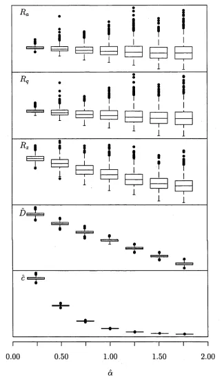
A numerical study was carried out to show how fractal methods perform in com parison with existing methods.

The three traditional roughness parameters i?a, R q and R z defined in Section 2.1 and the two fractal estimators D and c defined using the variogram method were calculated for a collection of simulated surface profiles. In calculating D and c, the one-dimensional empirical variogram (cf. 3.2) was used as an estimator of u(-), and

k was taken as 2.

Each simulated profile was a realisation of a stationary Gaussian random process with the stable exponential covariance model

7 M = 7(0) exp(—A|£|Q),

for its covariance function. Here, 7(0), the variance of the process, was set equal to the value 0.04 for all of the simulations. The simulations were performed using the algorithms in chapter 7.

Seven sets of 1000 profiles were simulated, each with different values for the pair (A, a). The a ’s took the values 0.25(0.25)1.75. The corresponding values for A were calculated so that the range of dependence within each process was approximately half the range of the data. To achieve this, A was calculated so that 7(0.5)/7(0) = e~3 « 0.05, which implies that A = 3 x 2Q.

Typical profiles for each pair of parameter values (A, a) are graphed in Figure

2.1.

Figure 2.2 contains 5 panels of boxplots, one panel for each of the roughness pa rameters discussed so far. Within each panel there are seven boxplots corresponding to the seven values of a. Each boxplot depicts the distribution of measures of 1000 simulated profiles.

(38)

[image:38.531.100.446.118.601.2]

(39)

T

0.00 0.50 1.00 1.50 2.00

a

[image:39.531.118.443.91.644.2]

(40)

only marginal when compared with the dramatic differences between boxplots for estimated fractal dimension and estimated topothesy.

In this instance, the difference in nature between profiles from the different mod els is exhibited in both the fractal dimension and the topothesy. Since topothesy is a linear functional, we could quite easily exaggerate the vertical scale of profiles from different models by certain factors so that their estimated topothesies were similar. It is comforting to know that this would have no effect on the estimate of fractal dimension, since it is scale-independent.

(41)

C h a p te r 3

T h e v a rio g ra m

All of the methods for characterising and comparing surface roughness developed

in this thesis are based on the variogram. Because the variogram plays such an

important role in these methods, it is fitting that a chapter be devoted to its study,

which addresses computational and stochastic properties of an appropriate estimator

for it.

There are a number of different estimators of the variogram; however for our

purposes the naive empirical variogram will suffice. Its limitations are mitigated by

the typical size of data sets in surface problems, and its benefits include mathematical

tractability, ease of computation (for which we provide computationally efficient al

gorithms), and its fam iliarity to various scientific and engineering groups, although,

in some cases, not as an estimator of the variogram.

The variogram and the auto-covariance function of a surface are similar in that

roughness properties that we wish to estimate can be derived from estimators of

either. However, there are a number of advantages in using the variogram over the

auto-covariance in this instance: it exists for a larger class of problems, it excludes

an unnecessary parameter, and its naive estim ator is unbiased.

We look at a few ways of displaying the variogram fo r one- and two-dimensional

data. Some of these graphs can provide useful inferences about the roughness

(42)

CHAPTER 3. THE VARIOGRAM 35

acteristics of a surface, such as isotropy or a dominant roughness direction.

The statistical properties of the methods depend heavily on properties of the em

pirical variogram as an estimator. We derive its moment properties and asymptotic

distributional behaviour in terms of the two roughness parameters, fractal index and

(43)

3.1 D e fin itio n

The variogram was defined in section 1.4 for an intrinsically stationary random process. More generally, the variogram for a random process X ( t ) may be defined as a function of two arguments, location t and displacement /i, by

v( t, h) — var [X(t + h) — X(i)].

From this definition, the following observation about v(t, h) may be deduced:

v(t, h) = v(t + h , —h). (3.1)

If X( t ) is intrinsically stationary then v(t , h) is independent of location and depends only on displacement. In this case we write it as v(h).

The simple observation (3.1) then becomes v(h) = v(—/i), that is, symmetry about the origin. This implies that when calculating or estimating v(t) from one dimensional data, one need only calculate v(t) for nonnegative values of t, and sim ilarly when estimating v(t) from two-dimensional data, one need only be concerned with t in a half-plane.

A necessary condition for the validity of variograms, in the sense that associated sample paths are real-valued, is that of conditional non-positive definiteness, that is, for any finite number of spatial locations t x, . . . , t mand real numbers c i , . . . , cm satisfying ci =

m m

-

1

,)

< o .

i=i j=i

In chapter 6 we explore the implications of this important property for fractal dimension and topothesy in the anisotropic two-dimensional setting.

(44)

3.2 E s tim a tio n

One of the simplest estimators of the variogram is the empirical variogram. Given a realisation of an intrinsically stationary random process X : Q —> R, the empirical variogram is defined as

and IC(h)\ > 1. For one-dimensional data, \C(h)\ = n — n\h\.

When dealing with gridded data, the domain of O(-) is itself a grid, centred at the origin. Thus, we can use perspective plots and similar graphical methods to explore its features.

The empirical variogram is also called the sample variogram in statistics, or the

structure function in other sciences. Interestingly, the structure function is already used in some areas of application to estimate fractal dimension, although the reasons for its use lack a theoretical basis.

There are other methods of estimating the variogram; see for example Cressie (1991). Most are concerned with robustifying the estimate against domination by a few summands in (3.2). When dealing with smaller non-gridded data sets (often the case in geostatistics) this is an important practical consideration. However, surface data sets are gridded and often large, implying that the number of summands | C(h)\

that go into estimating v(h) is large. The differences between different variogram estimators for such data are negligible. So, for mathematical convenience, we shall use the naive empirical variogram as our variogram estimator, although the methods developed are appropriate for other estimators too.

We shall see that point estimation of fractal dimension and other roughness parameters requires the variogram to be estimated at only a relatively small number of displacements. However, other methods presented, including the model fitting for simulation of section 4.3, require the variogram to be estimated over a large portion

(3.2)

t e c ( h )

where

(45)

of its domain, if not its whole domain. For this reason we provide a more efficient holistic algorithm for its computation.

One-dimensional algorithm

In the one-dimensional case,

n —|/i|

v(h) = ( n - |/i|)_1 ^ [ X ( t + \h\) - X { t ) } 2

t — 1

— ( n - \ h \ ) 1(5'ii|#l| — 2C\h\ + S2,\h\)

where

j n n - j

S \ , j = E jX 2 , S2,; = £ V u2, and C s = ' £ , X J C w ¥ i ,

U=1 U=j 1

for 0 < j < n. Here, {5ij} and {52,; }’s are sequences of partial sums and, assuming that they are calculated in an efficient manner and intermediate results are kept, will require 0(n) operations.

The quantity C j is recognisable as the discrete convolution of {Xj} with the

reverse of itself. Using the Fast Fourier Transform (FFT) to effect the convolution in the Fourier domain, we may calculate all of the Cj s in 0 ( n log n) time.

To avoid edge effects, embed the sequence of Xi s in a sequence of zeroes of overall length 2n: for 0 < j < 2n put

Y {Xj+i, ifO < j < n

I 0, otherwise.

It should be noted that {Xj} need only be extended to length 2n — 1, but we choose to extend it to a length of 2n, since algorithms for implementing the FFT perform better if the sequence length is a highly composite number.

(46)

Now, {C j} is the circular convolution of { Y j } with its reverse:

2n—1

C, = £ £

The computational complexity of a sequential algorithm is the maximum com plexity of its component stages. Hence, the one-dimensional empirical variogram may be computed in 0 (n lo g n ) operations, compared with 0 ( n 2) for direct compu tation.

Two-dim ensional algorithm

Although this is a direct extension of the one-dimensional algorithm, there is a significant difference: v(-) needs a half-plane rather than just positive values. The following method calculates v(h) for all displacements h in {1 — n, • • • , n — l} 2.

Because indices of arrays are usually nonnegative, we introduce the following notation to switch between the domain of v(-) and the indices of a two-dimensional array. Variables annotated with a prime, such as j', range over 1 — n , . . . , n and will be used for the domain of {)(•), whereas unannotated variables, such as j, range over 0 , . . . , 2 n — 1 and will be used to index arrays. Furthermore, the implicit relationship between a variable and its annotated counterpart is given by

if 0 < j < n if 0 < j' < n

if —n < j' < 0.

From (3.2)

v ( f , k') = [(n - 1/1)(n - \k'\)]~\Si m - 2Cjk + SUjk))

note the absence of primes on the subscripts — where

-2

u + j' ,v+ k'

u v u v