An approach to implementing a relational database system

IMPLEMENTING A

RELATIONAL DATABASE SYSTEM

H. G. Mackenzie

the rese

arch contained in this report is entirely my

own work.

26 November 1979

_{Hugh MacKenzie}

1. Introduction

2. The Relational Model

3. Other Relational Database System Implementations 3.2 PRTV

3.2 System R 3.3 INGRES 4. Sample ALF queries

5, Formal Specifications of ALF 5.1 ALF Syntax

5.2 Evaluation

5.3 Aggregate Functions 5.4 Nesting of queries

6. The Mapping between the Relational and Network Data Models 7. Transforming an ALF statement

7.1 Overview of Section 7 7.2 Query evaluation model 7.3 D-graph

7.4 Pattern Matching 7.5 V-graph

7.6 V-graph transformation

7.6.2 Coalesce equivalent nodes . _f

7.7 Use of V-graph in code generation i

7.8 Amalgamation of Equivalent Queries I

8. Code generation .I

8.1 Efficiency considerations 8.2 First pass

8.2.1 Finding Start Node and Initial Access Method

~

8.2.2 Subgraph Traversal and Access Method Extraction

J·

~

8.3 Second pass

~

8.3.1 Graph Traversal: Code Generation and Subquery Compilation

8.3.2 Currency and UWA usage

8.4 Boolean Test Generation in the presence of Subqueries

-8.4.1 Standard Boolean Test Generation

8.4.2 Introduction of Subqueries 8.5 Code optimisation

8.6 Final output 9. Extensions and Problems

9.1 Updates

9.2 Security and Integrity 9.3 More General Joins 9.4 Views

10. Conclusion Bibliography

Appendix A - Implementation Language

Appendix C - CODE-A, a sample target language Appendix D - Schema Specification

1.0 Introduction

Database management systems based on the CODASYL DBTG recommendations have become a de facto industry standard, and are available on the machines of most major manufacturers. These systems augment a higher level language such as COBOL, Fortran or PL/I with data manipulation commands, and hence using them requires programming an application in one of the host languages. This interface is at too low a level for the casual user. Many potential users are reluctant to make the initial heavy learning and programming investment required to use these systems effectively. In addition, the effort required after this initial investment, in programming each additional query, is considerable.

The situation would be vastly improved if the interface presented to the user was at a much higher level. The relational model, where the user views the data as a number of large tables, is one candidate for providing such a higher level interface.

In this paper, after giving a brief description of the relational model, I describe some currently implemented relational database management systems. Secondly, I describe the prototype implementation of a relational language, ALF, designed to act as a front end to a CODASYL database. ALF has been implemented as an interactive system at the CSIRO Canberra installation. It produces output in a language called CODE-A, and examples of the output may be found in Appendix E. This implementation involved setting up a mapping between the relational model and the CODASYL (network) model, and, from this mapping, deriving algorithms to translate commands in the relational language ALF into efficient programs suitable for execution on network databases.

The ALF translator may be regarded as a special purpose optimising compiler, as much attention has been paid to generating efficient code. The benefits of spending time on optimisation are even more clear cut with a database access language than with an ordinary programming language, as the programs being optimised are typically only a few lines long, and the extra time spent in translation can save many accesses to disc at execution time, in addition to saving central processor time.

As implemented at present, ALF does not contain any update commands, however their introduction would be straightfonvard, and the underlying algorithms would still be used if they were introduced.

The approach described in this paper has several novel features.

...---

---

- - - -- -- - - -- - -- -

---~

- - -- - · - - -- - - --- - ---- - - -- - - -- ·

--2

CODASYL set structure in implementing foreign keys, these keys are not explicitly stored. This would significantly increase retrieval efficiency, as well as introducing an important integrity constraint. 2) Implementing a relational interface to an existing database system allows the implementor to avoid most of the work which other

relational system implementors have had to face, for example file and

index structures, concurrent access, etc.

3) Although the network-relational correspondences have been pointed

out or alluded to on previous occasions, for example, in (Nijssen 1974), (Olle 1975), (Sibley 1974), translation algorithms developed from them have not been previously published, to my knowledge.

4) The translation process generates an intermediate language which may either be interpreted directly or translated into any (reasonable) target language. Whether the command is to be interpreted or compiled, and what the target language 1s to be, 1s determined by the interchangeable final pass plugged onto the translator. This feature allows the possibility of having a common interface to different

CODASYL Database Systems, perhaps running on different machines. The final pass currently included in ALF generates code in a language called CODE-A, which is described in Appendix C.

5) Unlike other relational systems, execution of a program generated by ALF does not involve the generation of any intermediate files: This contributes to increased retrieval efficiency.

The reader who simply wants some idea of the work described in this paper can read the sections 2 and 4, on "The Relational Model" and "Sample ALF queries'·.

These two sections are self contained. The section on "Formal Definition of ALF" contains some material oriented towards understanding the sections which follow on the translation algorithms.

This project would not have been· completed, or indeed started, without the encouragement and assistance of Dr J. L. Smith.

.

- -· .. · - - - -_ - - - -_- _-_--_--·--- ----·--- - - - · - - -· · · ·

-.

2.0

sys

·

the

. .. tog

anc

ear

inc

the

wa~ nur or:

a

t

coli

rela

De:

, I

r

There have been a great many articles published on Relational Database systems, thus only a brief and incomplete survey will be presented here. In particular, · the important topics of functional dependency and normalisation

will

not be covered.

The relational model of data was first proposed in (Codd 1970), a paper which, together with (Codd 1971a,1971b) produced a flood of research into Relational theory and practice. The Relational model used in this paper is the one described in Codd's

early

work; recent extensions, for example those described in (Codd 1979), are not ,.,

included.

Basically, the relational model describes a way in which a database user views

the data in a database. There is no requirement that this view shall correspond to the

way in which the data is stored. The data may be considered as being arranged in a number of tables or matrices, each one called a relation and given a name. Each. table

or

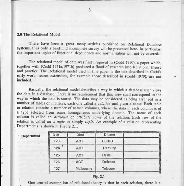
relation contains a number of named columns, where the data in each column is of a type selected from some homogeneous underlying domain. The name of each

column is called an attribute or attribute name of the relation. Each row of the relation is. called an n-tuple or simply tuple. An example of a relation representing Departments is shown in Figure 2.1.

"'

· _Department.

0#

Otoe Dname

123 ACT CSIRO

.

124 ! ACT Treasury .

125 ACT Health

126 ACT Defence

127 Melbourne Telecom

Fig. 2.1

One central assumption of relational theory is that in each relation, there is a

. subset of the attributes of the relation whose values uniquely identify the relation tuple

in

which they occur; that is, by appealing to the semantics of the system being modelled by tlie rclation:11 database system, it is known that two tuples may not haYe the same values of these identifying attributes. This constraint is assumed to be enforced by those programs which maintain the database. In addition, this subset is minimal, that is by removing an attribute from the subset, one destroys this uniqueness property. Such a subset of the attributes of a relation is called a candidate

key. A candidate key which never has any of its component attributes undefined is

[image:8.616.0.606.25.637.2]

-4

Fur a p:1rtil·t:l.1r :1ppliL":11i1i11. thL· 1t1t:tli1y of rcl:1ti1i11s :ind :1ttrih111L's c:111 he considered to modd tht.! application. This model is calkd a t\_•/otioncil schema.

A relation 111 a relational database may represent a cbss of objects (in the widest sense) in the real system being modelled by the database system. Two objects in the system may be related in some way. One way that relational database systems represent this is to have the identifying attributes (that is, the primary key or one of

the

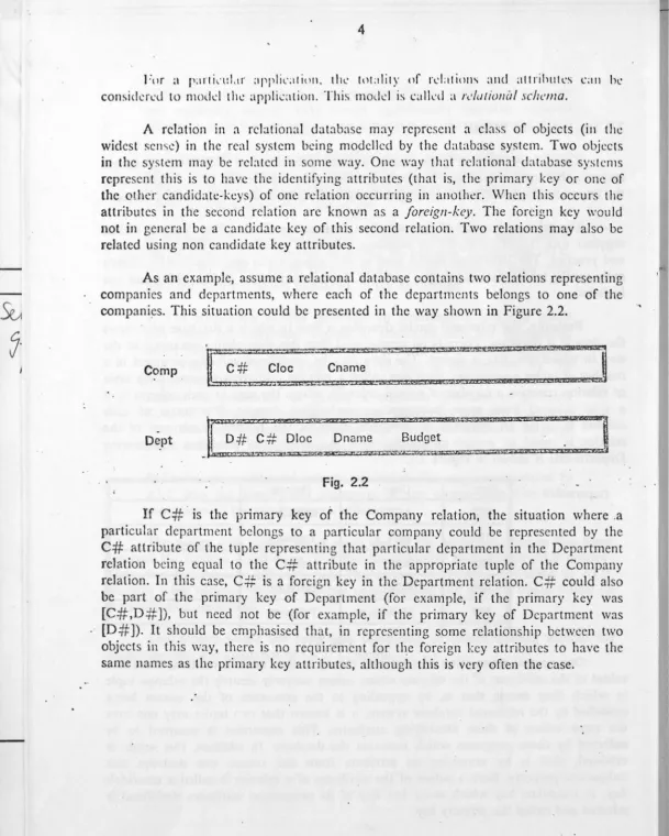
other candidate-keys) of one rdation occurring in another. Wht.:n this occurs the attributes in the second relation arc known as a foreign-key. The foreign key would not in general be a candidate key of this second relation. Two relations may also be related using non candidate key attributes.

As an example, assume a relational database contains two relations representing companies and departments, where each of the departments belongs to one of the compani~s. This situation could be presented in the way shown in Figure 2.2.

Comp

-Dept

Fig. 2.2

If

C# 1s the pnmary key of the Company relation, the situation where .a particular department belongs to a particular company could be represented by the

C#

attribute of the tuple representing that particular department in the Department relation being equal to the C# attribute in the appropriate tuple of the Company relation. In this case, C# is a foreign key in the Department relation. C# could also be part of the pnmary key of Deparlment (for example, if the primary key was [C#,D#]), but need not be (for example, if the primary key of Department was

.· [D# ]). It should be emphasised that, in representing some relationship between two objects in this way, there is no requirement for tl~e foreign key attributes to have the same names as the primary key attributes, although this is very often the case.

\

'

[image:9.649.10.619.13.773.2]

3. Other Relational Database System Implementations

This section first gives a classification of the types of language that have been proposed for manipulating data stored using the Relational Model, and secondly fits the methods used in the ALF implementation into context by describing some other Relational Database System Implementations. There have been many such implementations, and this report will mention only three of them, viz PRTV, System-R, and INGRES. The selection has been based on the fact that the systems described do not implement the operators specified in the relational language in a brute force, straightforward way, but make significant transformations and optimisations in translating from the operations at the logical level of the Relational language to the physical level at which the data is actually stored.

Languages for accessing data stored using the Relational Model have been classified in (Chamberlin 1976) under the following headings :

Relational Calculus Oriented Languages Relational Algebra Oriented Languages Mapping Oriented Languages

Graphics Oriented Languages

Natural English query langu?.ges could be added to this classification.

In Calculus oriented languages each relation may be thought of as a predicate in a first order predicate calculus, and each tuple may be thought of as a ground instance of such a predicate. A statement in a calculus oriented language contains a qualification which selects a subset of the tuples in the database. A targetlist selects attributes from the retrieved tuples, and a command operates on the selected values, outputting them or performing some other computation. The qualification is a formula in a first order predicate calculus, and may contain universal and existential quantifiers in some languages (Codd 1971 b ).

In Algebra Oriented languages a number of unary or binary operators are defined on relations, and produce new relations. These operators include Projection, Restriction (Filter, or Selection), Join, Division and the set operators Union, Intersection and Difference. There is an assignment operator, used to assign the result of a relational algebraic expres:;ion to an intermediate result relation, which may, in turn, be used in other expressions. Relational Algebra has been discussed in detail elsewhere, for example in (Codd 1972b), and will not be treated here.

6

Relational Algebra. An algorithm for this transformation is given in (Codd 1972b). The aloorithm "·as c!c,·clopcd with the aim of demonstrating the equivalence, independent of any implementation. The efficiency questions raised by this algorithm were adcJ rcsscd in (Palermo 1972).

Mapping Oriented languages are languages such as SEQUEL (Chamberlin 1974). They comprise nested mappings ; a mapping being a block of code which maps a known attribute or set of attributes into a desired attribute or set of attributes. The result of one such mapping may be used in specifying another mapping.

Graphics Oriented languages, of which Query-By-Example (QBE), (Zloof 1975, 1977), is the best known, operate by having the user fill in blank spaces in a predefined form, or blank relation.

It

is claimed in (Thomas 1975), that this approach facilitates learning to use a relational language. This assertion is less obviously true for more complex operations than for the simpler ones. In other ways graphics oriented, or tabular languages appear to be equivalent to relational calculus based languages, and translatable to thrm in a straightforward manner.

3.1 PRTV

PRTV, (Peterlee Relational Test Vehicle) is described in the series of papers by Hall and Todd, as well as in (Verhofstad 1976) and (Owlett 1976). It is a system developed at the IBM UK Scientific Centre at Peterlee, and has been used for some large applications. Its user interface, ISBL, (Information System Base Language), is based on Relational Algebra.

The underlying relational database files, called bricks, are stored sorted by leading attributes, common leading attributes being suppressed, and other attributes being compressed. Text values are stored in an area separate from the relation tuples themselves.

The algebraic operators union, intersection, difference, select, join and project are implemented at the ISBL level, and are specified in infix notation. There is an assignment operator. The ISBL expression is transformed to a language called CJL, (Common Intermediate Language). In this form the expression is called a cilstring, and is essentially the ISBL expression tree in a linearised, prefix notation.

The ISBL user may supply a numbe·r of assignment statements, any one of which may use the result of a previous statement. Relation names may be used as variable identifiers, or new variable identifiers may be introduced as a result of an assignment statement. Each time: an identifier is used, it is bound either by value or by name. If value binding 1s used, the current relation value 1s inserted into the expression. This is presumably done by copying the whole relation. If name binding is used, the relation name is inserted, and the relation tup es are materialised at the time the expres ion is evaluated. Name binding enables any changes to the database to be reflected in the answers to queries, and hence is used to define different views of the

---data. Then.: is another, less frequently used binding type, called binding by expression, which is described in (Owlett 1976).

The Algebraic operations in eayh statement are not carried out at the time that the statement is input, but are deferred until one of the following occurs.

a) The user lists a result relation.

b) The user asks the cardinality of a result relation.

c) The user requests that the result relation be explicitly materialised, and stored as a brick.

d) The user converts the result relation to a relational file . Relational

files allow a users program to access the relation as a sequential file, one tuple at a time.

When one of these op~rations occurs, the expression tree is optimised, and evaluated to produce the result tuples. The latest published status of the optimisation stage is given in (Verhofstad 1976). Verhofstad distinguishes two types of optimisation; global and local. Global optimisation deals with issues of database organisation, such as what indexes to maintain, and tuple placement control. These issues are discussed in (Hall 1975a).

Local optimisation is furthur divided into algebraic opttm1sations, which use relational algebraic identities to transform the query tree into an equivalent one, and non-algebraic optimisations, which transform the tree using such performance improving measures as file inversion. Local optimisation is discussed in (Hall 1975) and (Verhofstad 1976).

tree.

Local optimisation performs the following sorts of transformations on the query

• Filters (that is, selectors) are moved as far down the tree as possible. This causes them to be executed as early as possible, reducing the sizes of the relations that have to be handled.

* Multiple adjacent projections are merged into one projection.

• Projections which remove leading attributes, on which relations are sorted, require that the result be resorted, and are moved towards the leaves of the tree for earliest possible execution. This reduces the amount of data in each tuple that must be handled.

-8

transformed to a brick, and reaccessed when necessary.

* The most efficient implementation of the relational operators, particularly join, is estimated in a particular case. Indexes are used where possible.

* Idempotency laws for relational and boolean algebra are applied to simplify the expression.

* Various more complicated tree transformations, particularly involving the use of indexes, are applied. (see Verhofstad 1976)

Tree transformations similar to those used in PR TV are also discussed m (Smith 1975), in reference to the Relational Algebraic.system SQUIRAL.

After the tree is transformed, a process is associated with each relational operator, or internal node. Full materialisation, or realisation of intermediate files is avoided as much as possible. Each process on an internal node makes calls to the processes on the children of that _node to materialise a single result tuple. This tree of processes is similar to the List Set Generator method used in (Mackenzie 1977c). Realisation is necessary for some projections, where a file must be sorted to remove duplicates, and resorted using leading attributes as sortkeys. A node where a full realisation is necessary is called a break point .

3.2 System-R

System-R 1s one of the better known and most well developed Relational Database Systems. Its user interface language 1s SEQUEL (Chamberlin 1974). System-R consists of a Relational Storage System (RSS), whose Interface language is the Relational Storage Interface (RSI). The RSS is concerned with managing devices, space allocation and paging, locking, deadlock detection and backout, recovery, and with maintaining images and links, which are described later in this section.

On top of the RSS, and interfacing to it is a Relational Data System (RDS), which is accessed via au interface called the ReJ.ational Data Interface (RDI). RDI provides facilities closely parallel to those in SEQUEL, although it will also support other systems such as QBE (Zloof 1975, 1977). A programming language is interfaced

to the RDS using a cursor, which identifies a set of tuples called the active set of the cursor. One can associate a SEQUEL statement with a cursor, and retrieve tuples satisfying the statement into locations in the user program using a FETCH call.

The RDS contains an optimiser which chooses an algorithm to satisfy the query from the acce s methods supported by the RSS. It is this optimiser which is of most interest in this report.

-Relation tuples are stored in segments; and one segment may contain tuples

from a single relation or from more th:rn one relation.

Each tuple in a relation is identified by a tuple identifier , or TID. A TID

corresponds closely to a Database-key of CODASYL, being an efficient,

hardware-address oriented pointer to individual tuples.

The RSS makes explicit use of two structures, images and links.

An image is a B-tree index structure containing non-truncated keys. It provides fast access on a single attribute of a whole relation, and as the whole key is maintained in the index, can be used in retrieval without accessing the tuples themselves.

Leaf pages of an image are linked together in a doubly linked list.

Images may be clustering, in which case the tuples are maintained physically

sorted according to the image key, or nonclustering. It follows that there may be only

one clustering image for each relation.

An image resembles a SORTED, INDEXED, PRIOR PROCESSABLE set with OWNER SYSTEM, in CODASYL terminology. A clustering image corresponds

to the case where the record (relation) on which the image is defined has LOCATION MODE VIA the SET corresponding to the image.

A link is a mechanism for connecting tuples, and may be unary or binary. A unary link is a logical ordering on a· single relation, and resembles a SOR TED SET with OWNER SYSTEM, in CODASYL terminology. A binary link connects a single

tuple in one relation with all the tuples in another relation, such that the values of a particular attribute in the first, or parent, tuple equal the values of a particular attribute in the second, or child, set of tuples. A tuple participating in a link is joined,

· using TID pointers, to its prior and next twins in the link. Tuples must be inserted into a link individually at the RSS level. A link therefore resembles a MANUAL , non information bearing SET, where the SET membership is defined on the equality of certain data items in the owner and member records. Both types of link are PRIOR PROCESSABLE, in CODASYL terminology, as link members are connected with next and prior pointers.

Links and images may be created or destroyed at any time. The pointers which implement images and l"inks are TIDs and are stored as an affix to the tuple data. This affix may be expanded and contracted as images and links are created and destroyed.

-

-10

In summary, the storage structures used in System-R closely resemble a subset of those available in CODASYL systems, with the difference that in most CODASYL systems these structures cannot be created and destroyed.

The optimiser in the RDS begins by classifying the SEQUEL statement into one of several classes. The first class contains statements operating on a single relation, the second contains those containing a join term, and a third contains those which, in addition, use the GROUP BY option. Secondly, the optimiser examines the system tables to find images and links which could assist in executing the statement. Thirdly, a set of reasonable methods for executing the statement is derived, and lastly, cost estimates for each method are computed, and the method with minimum cost executed to produce a result.

For each relation, the system tables contain the following information.

R: The Relation cardinality.

D: The Number of data pages the relation occupies.

T: The average number of tuples per page (RID)

For each image, I, the image cardinality, (The number of distinct field values in the image), is maintained.

· A coefficient H, the number of tuple compansons equivalent to one page access, is estimated and stored.

Consider the case where there is a single relation query with a predicate containing a conjunctive term of the form (attribute) (relational-operator) (value). A number of cases arise. There may be no image, a clustering image, or a nonclustering image defined for the attribute. The relational operator may be "=" or not. The relation may occupy a file by itself, or there may be other relations in the file as well. To execute the query, either the whole relation may be scanned, or the image may be used. The properties of the predicate, together with the relation properties maintained in the system tables, are used to estimate the cost for one of eight methods for executing this type of query and to select one of them.

Consider a two relation query whose predicate contains a join term and a restriction on each relation in the query. There are a number of possible methods for evaluating such a query, usmg clustered or unclustered images on one or both relations, binary links between the relations, and whole relation scanning, possibly sorting the relations. A method is chosen which depends on the access paths actually available, and on whether the parts of the predicate involving one relation only are expected to be highly selective or not.

11

making calls to the RDS, and a result tuple produced incrementally wlh:ncvcr a FETC! I is done using that cursor. This avoids the generation of intermediate files.

3.3 INGRES

ING RES (Integrated Graphics and Retrieval System) was developed by Stonebraker and others at the University of California, Berkeley. It runs under the UNIX operating system on PDP 11 machines (model 34 or higher). The system is described in (Stonebraker 1976).

The user interface is via an interactive language, QUEL, which is calculus based, and allows aggregate functions to appear in the qualification. There is a version of QUEL callable from a higher level language. This version, called EQUEL, or Embedded QUEL, allows piped mode or tuple at a time retrieval into variables in a users program.

INGRES has an underlying storage structure which is paged, and in which each tuple has a TID similar to the TID in System-R, and similar to the CODASYL database-key. Five file structures are used. They are sequential or heap, hashed, compressed hashed, ISAM and compressed ISAM. Secondary indexes may be specified for any file. Each relation is stored as one such file, and there are no explicit links between files, except for those implied by the equality of attributes in different relations.

The hashed access methods provide retrieval given an exact value for the key attribute; ISAM in addition provides retrieval over a range of key item values.

The access methods all have a common interface, so that details of the access method's implementation is hidden from the higher level query execution processes. Adding a new access method is therefore straightforward, provided that it conforms to the existing interface conventions.

QUEL supports both retrieval and update, however only retrieval shall be explicitly considered here.

The query optimisation algorithms in INGRES operate by decomposing a query into a number of single variable queries. These queries are executed using a process called the OVQP (One Variable Query Processor). The reduced ranges are used in evaluating the residue of the query using tuple substitution. This process is similar to the process of pushing projections and restrictions back through joins in PRTV or in SQUIRAL (Smith 1975).

-12

them as a file indexed on a key to be used later in processing the residual query. After having evaluated those single variable queries that can be dctatched, the results of the evaluations are used to substitute attribute values in the residual query, creating a series of simpler queries. This process is equivalent to materialising the cartesian product of the reduced -ranges of the relations processed by the OVQP, and evaluating the residue of the qualification.

A more sophisticated decomposition algorithm is given in (Wong 1976), which gives an algorithm to be implemented in a later version of INGRES.

---4.0 Sample ALF statements

In this section I will show the capabilities of the calculus based relational language ALF which is the main topic of this paper. This will be done here using a set of example retrieval statements designed to demonstrate the language; A more formal definition will follow in Section 5. A larger set of example queries which were translated using the ALF translator, together with the output produced, is given in Appendix E. Syntactically the features of ALF are simil~r to, and to some extent modelled on, those of QUEL, although the underlying implementation, storage structures, and execution strategy is totally different.

4.1

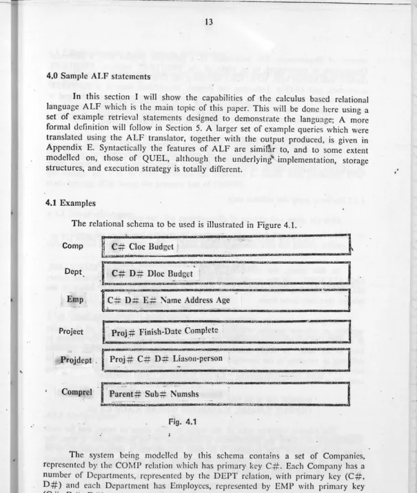
Examples

Fig. 4.1

The system being modelled by this schema contains a set of Companies, represented by the COMP relation which has primary key C# . Each Company has a number of Departments, repre~ented by the DEPT relation, with primary key (C#, D#) and each Department has Employees, represented by EMP with primary key (C#, D#, E#).

There arc Projects, represented by PROJECT with primary key PROJ

#.

Each Department may be associated with a number of Projects, and each Project with a

[image:18.632.16.621.17.732.2]

-,

14

number of Departments. The assoc1at1on of a particular Project with a particular Department 1s represented by a tuple of the PROJDEPT relation. PROJDEPT contains two foreign keys, (D#, C#) indicating the Department participating in the association, and PROJ # indicating the Project. In addition there is a SUPPLIER relation with primary key S#, a PART relation with primary key P#, and a

SUPPLY relation. The SUPPLY relation contains S# and P # as foreign keys. Each

tuple in the SUPPLY relation represents the fact that Supplier S# supplies Part P # .

Each of these sample retrieval commands will consist of a command, following

by a target/isl of attribute values to be retrieved and operated on by the command,

and a logical condition following the word "WHERE". This logical condition, or qualification, restricts the set of values returned in the target list.

4.1.1 Retrieval using one relation only.

Give the name and address of all employees who are over 60.

OUTPUT EMP.NAME, EMP.ADDRESS WHERE EMP.AGE GT 60

In this query, the command 1s OUTPUT, the targetlist 1s EMP.NAME, _ EMP.ADDRESS, and the qualification is EMP.AGE GT 60. The attribute names NAME, ADDRESS and AGE are qualified in this query by EMP, which is the relation that they come from.

In general however, attribute names m the target list are qualified by a variable, or relation variable, which may be thought of as ranging over all the tuples of a particular relation. Conceptually, the variable takes each tuple of the relation in turn as its value. In ALF, relation names do double duty as relation variables referring as variables to the corresponding relation. When a relation variable which is not a relation name is used, it must be declared in a RANGE statement before being used. Thus an equivalent way to express the previous query is

RANGE OF XIS El\1P.

OUTPUT X.NAME, X.ADDRESS WHERE X.AGE GT 60.

The relation variables take all the tuples in their range as value, and for each

combination of tuples, the qualification is evaluated. If the qualification is true, the targetlist is accepted. The targetlist is in some respects like a virtual relation, to be operated on by the statement command, except that there is not necessarily a primary

15

4.1.2 Retrieval using a join hetween two relation'>.

Give the name and address of employees who work for companies located in the ACT.

OUTPUT EMP.NAME, EMP.ADDRESS WHERE COMP.CLOC EQ "ACT"

AND COMP.C# EQ EMP.C# .

In this case the qualification reads " .. the company's location is "ACT" and the company's company number is the same as the employee's company number". The latter conjunct in the qualification is called a join term. Recall that the presence of the foreign key C# in EMP indicates the company to which each particular EMP tuple belongs (C# being the primary key of COMP).

4.1.3 Use of disjunction

Give the name and address of employees who work for companies which are either located in the ACT or which have budgets greater than ten million dollars.

OUTPUT EMP.NAME, EMP.ADDRESS WHERE COMP.C# EQ EMP.C#

AND [COMP .CLOC EQ "ACT" OR COMP .BUDGET GT 10000000].

4.1.4 Use of expressions in qualification

Give the department names of departments whose budgets are more than 20% of their companies budgets.

OUTPUT DEPT.NAME

WHERE DEPT.BUDGET GT 0.2 * COMP.BUDGET AND DEPT.C# EQ COMP.C# .

4.1.5 Multiple joins

Give the name and address of liaison people whose projects are not complete after the first of May, 1979, and who work for company XYZ, department ABC.

OUTPUT EMP.NAME, EMP.ADDRESS WHERE EMP.C# EQ "XYZ" AND EMP.D# EQ "ABC" AND PROJECT.FINISH-DATE LT 790501 AND PROJECf.COl\'IPLETE EQ "NO"

AND PROJECT.PROJ # EQ PROJDEPT.PROJ

#

1

16

AND PROJDEPT.D# EQ E1"IP.D#

AND PROJDEPT.C# EQ EMP.C# ..

4.1. 6 Introduction of aggregate functions in qualification

Find all departments whose budgets are greater than the average departmental budget (that is, the average for all companies).

RANGE OF Dl, D2 IS DEPT.

OUTPUT D1.D# WHERE

Dl.BUDGET GT A VG(D2.BUDGET) .

4.1. 7 Another example using an aggregate function

'

Find all departments whose budgets are greater than the· average departmental budget for their own companies.

RANGE OF D1,D2 IS DEPT.

OUTPUT Dl.D# WHERE _I

DI.BUDGET GT AVG(D2.BUDGET WHERE D2.C# EQ· Dl.C#) .

In example 4.1.6, D2 ranges over all tuples m the DEPT relation, and

computes the average budget. D 1 ranges over all tuples of the DEPT relation a second time, accepting those tuples which satisfy the qualification, that is whose budgets are greater than the previously computed average.

In example 4.1.7, Dl ranges over all the tuples of the DEPT relation, and for each tuple, the average is computed by D2 ranging over all the DEPT tuples which have the same C# as the Dl tuple. There is scope for optimisation here, but this optimisation is not the concern of the ALF user.

It is important to note that the text which follows the aggregate function A VG, is merely another query in the form

targetlist WHERE qualification

This query is evaluated, and the aggregate function applied to the collection of tuples which result from the evaluation. The number of items in the targetlist must equal the number of arguments expected by the aggregate function. Aggregate

functions currently available in ALF are MEAN, A VG, MAX, MIN, RANGE,

COUNT, TOT AL, SSQ, EXISTS, ALL.

These last two functions provide facilities equivalent to existential and universal quantification 111 the query qualification, and greatly extend the power of ALF retrieval statements. For a fuller description of these see Section 5.3, and the examples

- - - --- -

4.1.8 Use of two aggregates in retrie}·al statement

Find companies which have average departmental budgets less than 30000 or a maximum departmental budget greater than 100000.

RANGE OF Dl,D2 IS DEPT. OUTPUT COI\tlP.C# ·wHERE

MAX(Dl.IlUDGET \VHERE Dl.C# EQ COMP.C#) GT 10000000

OR AVG(D2.IlUDGET \VHERE D2.C# EQ COMP.C#) LT 30000.

In this example, the variable COMP ranges over the tuples of the COMP relation, and for each tuple, Dl and D2 individually range over all the DEPT tuples to compute the MAX and A VG aggregate functions. There is scope here for optimgation of the execution of this query, but again, this is not the concern of the ALF user .

.

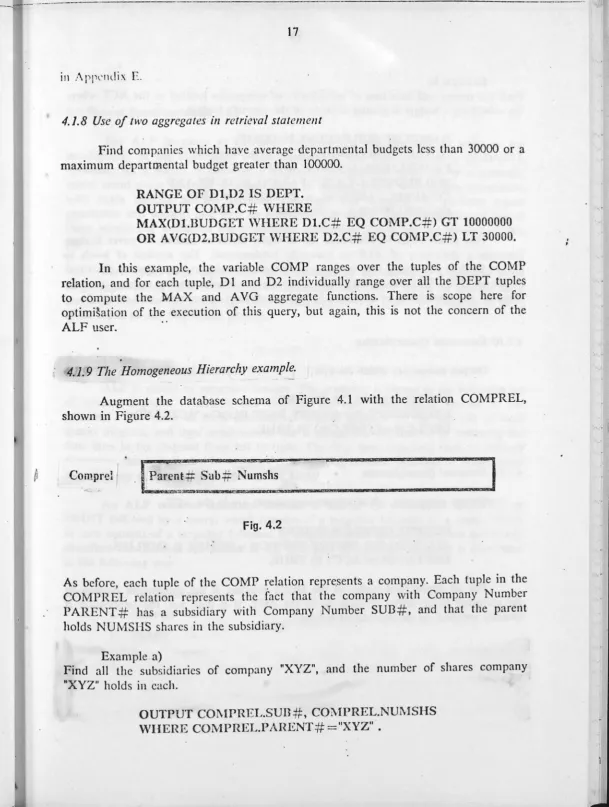
4.1. 9 The Homogeneous Hierarchy example.

Augment the database schema of Figure

4.1

with the relation COMPREL, shown in Figure 4.2.

I

Fig. 4.2

As before, each tuple of the COMP relation repre.sents a company. Each tuple in the COMPREL relation represents the fact that the company with Company Number PARENT# has a subsidiary with Company Number SUB#, and that the parent holds NUMSHS shares in the subsidiary.

Example.a)

Find all the subsidiaries of company "XYZ", and the number of shares company

"XYZ" holds in each.

[image:22.630.17.627.17.825.2]

-18

Example b) ·

Find the names and locations of subsidiaries of companies located in the ACT where the subsidiary's budget is greater than ¥i of the parent's budget,

RANGE OF SUB,PARENT IS COMP.

OUTPUT SUB.CNAl\lE, SUB.CLOC WHERE

PARENT.CLOC EQ "ACT" AND

SUB.BUDGET GT 0.75 * PARENT.BUDGET AND

COMPREL.PARENT#

=

PARENT.C# AND

COMPREL.SUB#

=

SUB.C#.

This process can be continued for as many levels as needed, however it does illustrate a deficiency of ALF as currently implemented. The number of levels is always fixed in the query, that is, there is no transitive closure operation as described in (Zloof 1976). This means that there is no mechanism for issuing a query such as "Find all the subsidiaries of company XYZ, and all their subsidiaries, and so on ... "

4.1.10 Existential Quantification .

Output companies which have at least one department located in the ACT.

OUTPUT COMP.C# WHERE

EXISTS(DEPT.D# WHERE DEPT.DLOC="ACT" AND

DEPT.C# =COMP.C#) IS TRUE.

4.1.11 Universal Quantification

Output companies, all of whose departments are in the ACT.

OUTPUT COMP.C# WHERE

-ALL(DEPT.D# WHERE DEPT.C# =COMP.C# IMPLIES

DEPT.DLOC="ACT") IS TRUE.

For all department tuples in the DEPT relation, if the department belongs to the company being tested, it must be in the ACT. If it does not, the implication is trivially satisfied, as the antecedent is false.

The EXISTS and ALL functions are really predicates over one or more

relations, rather than functions over attributes selected from relations. Only the variables in the targetlist are significant, not the attributes. EXISTS is true if there is a combination of the targetlist variables which satisfies the qualification. ALL is true

·

if

the qualification is satisfied for all possible targetlist variable combinations.

-

-

~-

--- .,.

'

~ '

19

5.0 Formal Specification of ALF

The ALF language as currently implemented was designed to assist in the development of the algorithms which translate it into operations on a CODASYL database. As it stands it contains a statement for retrieval only. To be a generally useful stand alone language it would have to be augmented with update commands, with extra options on the retrieval command (for example, to perform report generation and sorting) and with an interactive capability. The introduction of any of these would not invalidate the translation algorithms which are the subject of this paper.

Nor would these algorithms be invalidated by the choice of a different input language; although ALF is based on the relational calculus, it would be possible for a language based on relational algebra or a language such as Query by Example to serve as an input to this ~ranS'lat1on process.

5.1 ALF Syntax

ALF is parsed by recursive descent. The grammar is shown in the following set of syntax diagrams. There is one· diagram for each nonterminal symbol in the grammar. The name of each nonterminal symbol appears on the top left of each syntax diagram, and legal constructs in the language are constructed by following the flow lines in the diagram from left to_ right. The flow lines may loop back to indicate repetition; this is indicated by appropriately pointing arrows. Terminal or nonterminal symbols may appear in the diagram.

An ALF retrieval statement consists of one of the comma,nds OUTPUT or PRINT followed by a query, which consists of a targetlist followed by a query, which in turn consists of a targetli~t followed by a qualification clause. Using the previously described conventions, the syntax of the first part of retrieval statement is illustrated in the following way

retrieval statement

+-OUTPUT-+

--+

+----+-PRINT--+

The full syntax follows

query---.

-'I

-20

statement

+----1

range statement ----+

I

---+

+---

-

---

-

----I

+-- retrieval statement--+ 1

range statement

-- RANGE -- OF -- variable list - IS - relation list retrieval statement

+-OUTPUT-+

--+ +---- query--- .

+-PRINT--+

query

-targetlist-qualification

clause---targetlist

+---

---+

t

.

I

---expression---qualification clause

-WHERE boolex ---boolex

+--- IMPLIES ----+

t

implicand

I

impl icand

+---OR---+

________ ±_

disjunct ___

l

______

_

disjunct

+--NOT--+

I

I

+---+----AND---+

1

I

---conjunct---conjunct

+--- [ boolex ] ---+

I

I

-----

term---r,

term

expression

aterm

afactor

aprimary

expression

21

+---

EQ

---+

I

I

+---

NE ---+

I

I

+---

GT

---+

I

I

+--- GE

---+

I

I

LT -expression

--1 I

+---LE---+

I

I

+---IS---+

I

I

+----EQUALS----+

I

I

+---

=

---+

I

I

+---

<

---+

I

I

+---

>

---+

+---- + ----+

I

I

+---- - ----+

t

I

--- aterm

+---- * ----+

I

+---- I ----+

I

t

afactor

I

+---- ** ----+

'

I

V

--- aprimary

I

--- item

---I

·

f · 1 ·

I

+-- ar1th- unction - (-arg 1st-)---+

I

I

+---

subquery

---+

I

I

+---

numeric constant---+

I

I

+---

logical constant---+

I

I

+---

string constant---+

I

.

I

+---

(

---

expression --- )

---+

·,·

-1 .

22

subquery

aggregate-function - ( -- query -- )

agregate-function

•

item

arglist

---AVG---+- MAX -+

+- MIN -+

+- MEAN-+

+-TOTAL -+

+-RANGE-+

+- SUM -+

+- SSQ -+

+-EXIITTS--+

+- ALL -+

+- SUM -+

+- SSQ -+

+- SD -+

relation variable . attribute name

-+--- ---+

t

.

I

---expression---arith-function

---+-

SIN

-+---+-

cos

-+

+- TAN -+

+- -+

Informally, the target list consists of expressions built up from items, which are

dotted pairs consisting of a relation variable and an attribute name. The relation variable must either be a relation name or must have been previously declared in a

RANGE statement. The relation referred to by a particu ar relation variable is called the range of that variable. Each relation variable may be thought of as taking a tuple from it's relation as it's value. The attribute name must be an attribute name in the relation referred to by the relation variable. The item pair selects the attribute value

from the relation tuple which is the current variabl~ value.

The qualification consists of a logical expression built up by using the logical operators AND, OR, AND NOT and IMPLIES. The precedence implied by the syntax diagrams may be altered by use of brackets in the usual way.

Terms consist of expressions connected by relational operators. Terms of the form R l.D l relational operator R2.D2 are called join terms; and those join terms where the relational operator is EQ play a special role in that they are (usually) used to connect one relation with another, and may allow one of the relations to be

23

Expressions are composed of items of the form relarion variable . attribure name, linked in the usual way using arithmetic operators and arithmetic functions. The variable in an item is said to qualify the attribute. The value of an item is the value of the named attribute in the relation tuple which is the current value. of the variable.

-

-

.

Each term may be thoughtof as a function of the relation variables in it, taking the values true or false.

5.2 Evaluation

The evaluation of an ALF command may be visualised in a number of ways. The following way, taken from (Codd 1972b) but omitting the steps concerned with universal and existential quantification, will be used in this paper.

1) Take the cartesian product of the ranges of all the relational variables which occur in the query.

·

rr

two or more variables range over the same relation, then that relation will occur in a cartesian product with itself in the final product. The cartesian product, sometimes called full

quadratic join, is as defined in (Codd 1972b ).

2) Reject those tuples in the cartesian product for which the qualification is false. If the qualification contained subqueries it would be necessary to invoke this evaluation process recursively to evaluate the query contained in the subquery, and hence to evaluate the qualification. 3) Project the result of 2) onto those items which occur in the target list. This projection does not eliminate duplicate tuples, but removes those items not specified in the target list.

4) Compute any expressions in the target list for each remaining tuple.

5.3 Aggregate Functions

In

general, a command may contain Aggregate Functions, which operate over the tuples retrieved by the associated query. Duplicate tuples are not removed before evaluation of the aggregate function, unlike some other relational languages.

24

1) MEAN, AVG

Compute the mean of the values of the targetlist expression.

2) MAX, MIN

Compute the maximum or minimum of the values of the expression in the targetlist.

3) RANGE

Compute the difference between the maximum and minimum values for the expression in the targetlist.

4) TOT AL, COUNT

Compute the total number of tuples returned as a result of the following query.

5) SUM

Compute the sum of the values of the targetlist expression.

6) SSQ

Compute the sum of the squares of values of the targetlist expression.

7) SD

Compute the standard deviation of the values of the targetlist expression.

8) EXISTS

This function returns the bool.~an constant TRUE if there are any tuples satisfying the qualification of the query governed by the EXISTS function. If no tuples satisfy the qualification, FALSE is returned.

9) ALL

The ALL function has a single argument. Let the argument be the item RV.DI, and let the range of RV be R. The function returns TRUE if all the tuples in the R relation satisfy the qualification, otherwise it returns FALSE. For example, the following would be TRUE if all employees in the database were under 50 years old.

ALL(E1VIP.E# WHERE EMP.AGE LT 50)

5.4 Nesting of queries

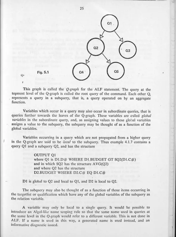
The qualification of the subquery may itself contain other subqueries, and so on, although more than two levels would be unusual. This leads to a hierarchy of queries in a statement, which may be represented graphically as in Figure 5.1.

25

Fig. 5.1

I

This graph is called the Q-graph for the ALF statement. The query at the topmost level of the Q-graph is called the root query of the command. Each other Q; represents a query m a subquery, that is, a query operated on by an aggregate function.

Variables which occur in a query may also occur in subordinate queries, that is queries further towards the leaves of the Q-graph. These variables are c:1lled global

variables in the subordinate query, and, as assigning values to those glo'.)al variables assigns a value to the subquery, the subquery may be thought of as a function of the global variables.

Variables occurring in a que1y which are not propagated from a higher query in the Q-graph are said to be ,focal to the subquery. Thus example 4.1.7 contains a query Q 1 and a subquery Q2, and has the structure

OUTPUT QI

where Ql is Dl.D# WHERE Di.BUDGET GT SQ2(Dl.C#) and in which SQ2 has the structure AVG(Q2)

and where Q2 has the structure

D2.BUDGET WHERE D2.C# EQ Dl.C#

D 1 is global to Q2 and local to Q 1, and D2 is local to Q2.

The subquery may also be thought of as a function of those items occurring in the targetlist or qualification which have any of the global variables of the subquery as the relation variable.

A variable may only be local to a single query. It would be possible to introduce an Algol-like name scoping n1le so that the same name used in queries at the same level in the Q-graph would refer to a diITcrent variable. This is not done in ALF. If a name is used in this way, a generated name is used instead, and an informative diagnostic issued.

[image:30.633.38.628.19.816.2]

-\

6.0 The I\1apping Ilctwcen the Relational and Network Data J\fodels

The first step in defining this mapping is. to set up a .correspondence between a

relational and a network schema which may be used to derive an equivalent network schema from a relational schema, and vice versa. Such a correspondence is suggested

in

(Olle 1975). A starting point is to set up the following fairly obvious

correspondence between CODASYL Records and Relations, and CODASYL Data

Items and Relation Attributes.

Network Term _{Relational Term}

-t· . . .

+

Record Type

Record Instance Data item in record

Relation name

tuple of relation Attribute in relation

+

...

+

Before defining the correspondence, note that the word coset is used throughout the rest of this paper to mean set in the CODASYL sense, following (Nijssen 1975).

A relational schema may be derived from a network schema by applying the following two steps.

1) Starting at the top of each hierarchy (at each record which is not

a

member of a non SYSTEM owned coset), propagate the primary key of each record down through the coset making it a data item of the member record of the coset. If data items propagated in this way are actually stored in t.he member record, the coset is said to be non information bearing (Metaxides 1975). If the data items are not stored

in

the record, but are implicitly defined by the coset, the coset is said to be information bearing, and the data items .are called 1•irtual data items. This propagation may be continued dov,in a hierarchy of cosets if necessary, virtual attributes being used as source attributes. This is done for each· hierarchical path in the network schema.

2) Define a relation corresponding to each record type, and define

attributes of the relation corresponding to the data items of the record. Virtual data items in the network schema become attributes in the rclation:.il schema. They arc called virtual allributes. The user at the relational level need not be aware that the virtual attributes arc not

In this paper, all coscts arc information Gearing. If a cosct i~ 11011 informatio,i bearing in the original network schema, that is, data items exist in the owner and member records whose equality defines the cosct occu·rrence in the schema, then those

data items must become virtual items in the member record.

The correspondence between a coset in a network schema and the equality between a primary key and a foreign key in a relational schema is the lynchpin of the

whole translation process used in ALF.

The reverse transformation from a relational schema to a network schema may

be carried out by identifying foreign keys in relations and defining a coset between

that record as member, and the record containing the foreign key as its primary key as owner. Foreign key names need not be the same as the names of the corresponding

primary keys, although, conventionally, they often are. Foreign keys must be chosen

with the semantics of the underlying data in mind.

Comp Fig. 6.1

... ~;,, .. ~"'--,11>."- ~ .. ~ ... "l

C#

t---~

~

.. ·- : -,,,."-"'"'"'""'.'""""•~

.

.

.

·

)!---,

B.ffi,,:;ill'.,:;.:.a;"..&£J.

rJJ

Dept S1 SS2

-

-

-~~Y

-~

]

·~°l..\.).''i...£~ ~~ ~ I.

·, '

.

,

.

-~t"':m.kr&~~':filj

S2 $3

. .

Project

~~

;;~

~~~WL

TI

L--=,,,.J

S4

Each chosen foreign key becomes a virtual data item 111 the member record of the derived coset.

[image:33.666.0.626.18.808.2]

Diagram, is called the C-graph of the network schema in this paper. The C-gr:1ph for the database used in the Ex·amplcs in Section 4 is r,iven in Figure 6.1, gi,·cn that tl10,e data items with the same names as primary keys of other records were chosen :1'i the

fo_rcign keys.

The network entity which corresponds most closely to the relational variable in ALF is a variable which takes a database key as its value. A database key docs in fact identify a network record occurrence, corresponding to a relation tuple, at least inside a single run-unit. The database key variable must be constrained to refer to one type of record only.

Thus, three extra correspondences are added to the table given earlier in this section

Network Term _{Relational Term}

+

...

...

...

+

Coset

Database key variable

Primary key - foreign key correspondence

Relation va1iable.

virtual data item Foreign key or virtual attribute

+

...

-

.

";

·

.,·

. .

.

. . .

.

.

.

. .

. .

. . .

.

. . . +

In the following sections the terms that have been defined as being in correspondence

will

be used somewhat interchangeably; the meaning will be obvious from the context.

'\

•

7.0 Transforming the ALF Statement

7.1 Overview of Section 7

The following section will describe the translation algorithms and demonstrate their validity. First the model for query evaluation in ALF initially given in Section 5.2 will be specified. Secondly a model for network databases using an equivalent structure called a D-graph will be described. Thirdly a graphical pattern, called a V-graph, after a similar structure defined in (Palermo 1974), will be derived from each query, and matching this pattern against the database D-graph will be shown to be equivalent to the original model for query evaluation. Fourthly, transformations will be defined on the V-graph, and it will be shown that each transformation produces a V-graph equivalent to the previous one in the sense that the set of answer tuples produced by matching it against the D-graph is unchanged by the transformation. Lastly it will be shown that the pattern matching process corresponds to CODASYL network traversing algorithms.

The translation algorithm may be divided into the following steps:

1) Input and preprocess the ALF statement.

2) Remove virtual attributes from each query.

3) Coalesce equivalent V-graph nodes.

4) Amalgamate equivalent queries.

5) Process each V-graph, starting at the V-graph corresponding to the root query of the Q-graph.

6) Optimise the generated code.

7) Either interpret the optimised code, or use it to generate statements in the required target language.

In step 1, the ALF statement is parsed and put into an internal form. Before the main part of the statement translation, two preprocessing steps are done.

The first of these converts each occurrence of the aggregate function ALL into an occurrence of the EXISTS function. This is done by applying the identity

ALL X WHERE B(X, .. )

<

=

>

NOT EXISTS X WHERE NOT BC', .. )

,·

to each subquery acted on by an ALL function.

The second preprocessing step removes references to virtual relations, or views. (See Section 9 .4)

Step 5, processing the query, is carried out for each subquery as well. This step may be divided as follows:

Sa) Find a starting node in the V-graph and an initial access method. Sb) Determine node accessing order and access methods for each node. Sc) Generate intermediate code for the query (This step will involve the processing of subqueries)

If the V-graph is disconnected, steps 5a and Sb will be repeated for each

disconnected subgraph.

7 .2 Query Evaluation Model

As described in Section 5, a query in ALF is an object of the form

targetlist WHERE qualification

Evaluation of a query is a process which produces a set of targetlist tuples. If

the query is part of a subquery, then these tuples will be operated on by a aggregate

function to produce a scalar value, and if it is part of a command, they will be

operated on by the command to produce some sort of output.

As described in Section 5, an ALF query may be thought of as being evaluated

by a four stage process.

1) If LV1, ••. ,LVn are the local variables in a query, and R

1, •••• ~ are

their respective ranges, take the cartesian product of the relations R₁ •••

R0 • If there are global variables GV_{1, •••} ,GV m in the same query, then

each time the query is executed, each global variable will have as value

a tuple Trom a relation in a higher level query. These tuples TGV 1 TGV m are concatenated to each tuple of the cartesian product.

Thus, the cartesian product has the following form:

LV1 LV₂

+---+ +---+

Ri[ 1] Rd 1]

R1[2) X R₂[2] X

Ri[ 3 J R₂ [ 3]

GV1

+---+

TGV₁

As the cartesian product contains every possible combination of tuples from its component local variable relations, the cardinality of the cartesian product will be the product of the cardinalities of each local variable relation. Materialising such a huge relation is out of the question, for efficiency reasons.

2) The query qualification is evaluated using attribute values from each tuple in the cartesian product. As the qualification is a boolean expression of terms containing items of the form variable.attribute, each column in the cartesian product must be labelled implicitly with the attribute name and the relation variable from which it was derived. All tuples for which the qualification is false are rejected, and all for which the qualificiation is true are retained.

3) The remaining tuples are projected onto those items which occur in the query targetlist, that is, items not participating in the targetlist are ignored.

4) The targetlist expressions are computed from the items in the tuples that remain.

5) If the query occurs as part of a subquery, the aggregate function of the subquery is applied to the resulting tuples, and if the query occurs as part of a retrieval statement, the statement command is applied to the resulting tuples.

There are several noteworthy features of this algorithm.

The first is that the process contained no operation occuring between tuples of the cartesian product, and so if each tuple of the cartesian product could be materialised one at a

time,

the qualification could be evaluated and that tuple accepted or rejected before materialising the next tuple.

The second is that if the cartesian product tuples could be produced incrementally in the sense that only one extra relation was multiplied into the cartesian product at once, and if the qualification could be factored into conjuncts of the form Q

=

factor AND residue, where factor contained items from those parts of

the tuple already materialised, then further relations need only be multipled into the cartesian product if the part so far materialised satisfied the boolean expression factor.

The most obvious case of this is where tuples from a single relation would not enter the cartesian product if they did not satisfy a conjunct in the qualification referring only to a relation variable with that relation as range.

C.

J

7.3 D-graph

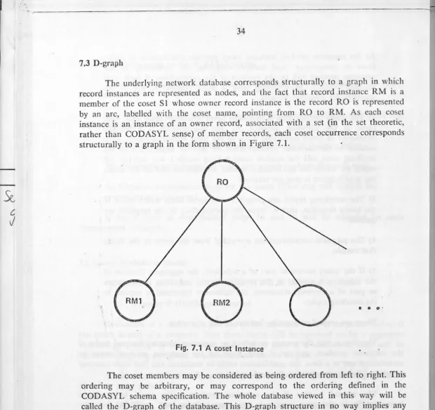
The underlying network database corresponds structurally to a graph in which record instances are represented as nodes, and the fact that record instance RM is a

member of the coset SI whose owner record instance is the record RO is represented by an arc, labelled with the coset name, pointing from RO to RM. As each coset

instance is an instance of an owner record, associated with a set (in the set theoretic, rather than CODASYL sense) of member records, each coset occurrence corresponds structurally to a graph in the form shown in Figure 7.1.

• • o•

Fig. 7.1 A coset Instance

The coset members may be considered as being ordered from left to right. This ordering may be arbitrary, or may correspond to the ordering defined in the CODASYL schema specification. The whole database viewed in this way will be called the D-graph of the database. This D-graph structure in no way implies any particular physical implementation.

Operations on this graph corresponding to CODASYL DML operations may

[image:39.656.5.625.15.599.2]