Rochester Institute of Technology
RIT Scholar Works
Theses
Thesis/Dissertation Collections
2002
Efficient Utilization of Fine-Grained Parallelism
using a microHeterogeneous Environment
William L. Scheidel
Follow this and additional works at:
http://scholarworks.rit.edu/theses
This Thesis is brought to you for free and open access by the Thesis/Dissertation Collections at RIT Scholar Works. It has been accepted for inclusion
in Theses by an authorized administrator of RIT Scholar Works. For more information, please contact
Recommended Citation
Efficient Utilization of Fine-Grained Parallelism using a
microHeterogeneous Environment
by
William L. Scheidel
A Thesis Submitted
III
Partial Fulfillment of the
Requirements for the Degree of
Master of Science
III
Computer Engineering
Primary Advisor: _ _ _ _ _ _ _ _ _ _ _ _ _ _ _ _ _
_
Dr. Muhammad Shaaban, Assistant Professor
Committee Member: _ _ _ _ _ _ _ _ _ _ _ _ _ _ _ _ _
_
Dr. Andreas Savakis, Associate Professor
Committee Member: _ _ _ _ _ _ _ _ _ _ _ _ _ _ _ _ _
_
Dr. James Heliotis, Professor
Department of Computer Engineering
Kate Gleason College of Engineering
Rochester Institute of Technology
Rochester, New York
Release Permission Form
Rochester Institute of Technology
Efficient Utilization of Fine-Grained Parallelism using a
microHeterogeneous Environment
I, William L. Scheidel, hereby grant permission to the Wallace Library of the
Rochester Institute of Technology to reproduce this thesis, in whole or in part, for
non-commercial and non-profit purposes only.
William L. Scheidel
ABSTRACT
Heterogeneous computing
environments use an assortment ofhigh
performance machines with
different
architecturesin
an attemptto
mostefficiently
executethe
varioustasks that
are requiredby
an application.While
this
environmentis
very
well suitedfor
tasks
such asimage
understanding,
heterogeneous
processing
has
key
limitations
which
including
the
lack
of supportfor fine-grained
parallelism, the
high
communication
overhead ofmoving
tasks
between
machines,
andthe prohibitively
high
costs.The
goal ofthis thesis
is
to
propose a newcomputing
paradigm,
calledmicro-Heterogeneous computing
ormHC,
whichincorporates PCI
(or
otherhigh
speedlocal
system
bus)
based
processing
elements(vector
processors,
digital
signalprocessors,
etc) into
a general purpose machine.In
this
mannerthe
benefits
ofheterogeneous
computing
on scientific applications canbe
achieved whileavoiding
some ofthe
lim
itations.
Overall
performanceis increased
by
exploiting
fine-grained
parallelism onthe
most efficient architectureavailable,
whilereducing the
high
communication overhead
and costs oftraditional
heterogeneous
environments.Furthermore,
mHCbased
machines can
be
combinedinto
acluster,
allowing both
the
coarse-grained andfine
grained parallelism
to
be
fully
exploitedin
orderto
achieve even greaterlevels
ofperformance.
An
existing
high
performancecomputing
API
(GSL)
was chosen asthe
interface
to the
systemto
allowfor
easy
integration
with applicationsthat
werepreviously
developed
using this
API.
The
ensuing
chapters will providethe
motivationfor
this work,
an overview ofheterogenous
computing,
andthe
details
pertaining to
microHeterogeneous computenvironment will
be
examined as well asthe
results.Finally,
the
future
of microTABLE OF CONTENTS
List
ofFigures
vList
ofTables
viAcknowledgments
viiGlossary
viiiChapter
1:
Introduction
1
Chapter
2:
Heterogeneous
Computing
5
2.1
Background
.5
2.2
Task
Scheduling
9
2.2.1
Segmented
Min-Min
10
2.2.2
Relative
Cost Algorithm
.12
2.2.3
Heterogeneous-Earliest-Finish-
Time
andCritical Path
on aPro
cessor .... . . . ... .14
2.2.4
Other
Mapping
Heursitics
18
2.3
Programming
19
2.3.1
Parallel Virtural Machines
(PVM)
19
2.3.2
Message
Passing
Interface
(MPI)
. . ....20
2.4
Limitations
....21
Chapter
3:
Application Program Interfaces
23
3.1
Background
. .233.2.1
Basic Linear
Algebra Subprograms
(BLAS)
24
3.2.2
Vector.
Signal,
andImage
Processing Library
(VSIPL)
...25
3.2.3
GNU Scientific
Library
(GSL)
... .28
Chapter
4:
microHeterogeneousComputing
30
4.1
Description
30
4.2
mHCAPI
32
4.3
Example
Devices
33
4.3.1
XP-15
34
4.3.2
Pegasus-2
35
4.4
Comparison
to
Heterogeneous
Computing
... .37
4.4.1
Task
Granularity
37
4.4.2
Task Execution
Overhead
38
4.4.3
Cost
Effectiveness
...39
4.4.4
Analytical
Benchmarking
andProfiling
40
4.4.5
Scheduling
Algorithms
40
Chapter
5:
microHeterogeneousComputing
Framework
42
5.1
Usage
42
5.1.1
Initialization
Parameters
. . ...42
5.1.2
Configuration
44
5.2
Implementation
. . ....46
5.2.1
Overview
. .46
5.2.2
Initialization
... ...46
5.2.3
Task Creation
... .50
5.2.4
Task
Scheduling
. .52
5.2.5
Task Execution
...52
5.3
Scheduling
Heuristics
. . ....53
5.3.2
Real-Time Min-Min
....55
5.3.3
Weighted
Real-Time
Min-Min
57
Chapter
6:
Results
59
6.1
Methodology
59
6.2
mHCSimulator
. . . .61
6.3
Application
Simulations
. . .62
6.3.1
Matrix
.62
6.3.2
Stats
. .64
6.3.3
Linalg
66
6.4
Scheduler
Performance
Comparison
67
Chapter 7:
Conclusions
74
7.1
Accomplishments
. . . .74
7.2
Limitations
. ... . ...75
7.3
Future Work
76
Appendix A:
Complete
mHCAPI
78
A.l
mHCSpecific
Functions
78
A. 2
Matrix
Operations
....78
A. 3
Vector
Operations
79
A.4
Polynomial
Solve
80
A. 5
Permutations
80
A. 6
Combinations
81
A.7
Sorting
81
A. 8
Linear
Algebra
.81A. 9
Eigenvectors
andEigenvalues
. .83
A. 10 Fast Fourier Transforms
. . . .84
A. 12
Statistics
...86
Appendix
B:
Sample Configuration
Files
87
B.l
Device Configuration
. . . .87
B.2
Bus
Configuration
89
Appendix
C:
Sample
mHCApplication
90
Appendix D:
mHCFramework
Source
Code
92
Appendix E:
mHCSimulator Source Code
93
LIST OF FIGURES
1.1
A Cluster
of microHeterogeneousComputers
.3
2.1
A Heterogeneous Environment
6
2.2
Code-Type
Profiling
Example
. . .8
4.1
A
microHeterogeneousEnvironment
31
4.2
The XP-15 DSP Accelerator
Card
34
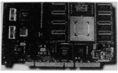
4.3
The Pegasus-2 Vector
Processing
Accelerator
Card
[6]
.36
5.1
microHeterogeneousComputing
Framework
...47
6.1
Matrix Application: Performance
vsNumber
ofDevices
...63
6.2
Stats
Application: Performance
vsNumber
ofDevices
.65
6.3
Linalg
Application: Performance
vsNumber
ofDevices
.66
6.4
Performance
ofRandom
Task Graphs
on aUniform
Set
ofDevices
. .69
6.5
Performance
ofRandom Task
Graphs
on aNon-Uniform
Set
ofDevices
70
6.6
Performance
ofRandom Task
Graphs
for
Increasing
Bus Transfer
Times
71
LIST OF TABLES
3.1
Example
ofVSIPL Blocks
andViews
27
3.2
Summary
ofVSIPL
Functionality
27
3.3
Summary
ofGSL
Functionality
. . .29
4.1
Scientific
Areas
Supported
by
the
mHCAPI
33
4.2
Comparison
ofthe
XP-15
and a1.4
GHz
Intel P4
[23]
35
4.3
Pegasus-2
Sample
Operation Performance
[6]
37
6.1
Matrix
Simulation
Data
Summary
.64
6.2
Stats Simulation
Data
Summary
. .65
6.3
Linalg
Simulation Data
Summary
67
6.4
Uniform
Set
ofDevices Performance Data
68
6.5
Non-Uniform
Set
ofDevices Performance Data
70
6.6
Increasing
Bus Transfer Times Performance Data
71
ACKNOWLEDGMENTS
I
wouldlike
to thank
everyone who supported orhelped
mein any
way to
completethis thesis:
Dr. Muhammad
Shaaban
-For
the
idea
of microHeterogenousComputing
andallowing
my to take
partin
it.
Dr. Andreas
Savakis
-For
providing
help
and counsel whenneeded.Dr.
James Heliotis
-For
being
a part ofmy
committee.My
family
-For
GLOSSARY
ANALYTICAL
BENCHMARKING:
Process
ofdetermining
the
suitability
of a partic ular machineto
execute a particulartask
CPOP:
Critical
Path
on aProcessor
Scheduling
Heuristic
ETC:
Estimated
time to
completion.The
estimated amount oftime that
a particular task
will requireto
execute on a particulardevice.
HEFT:
Heterogeneous-Earliest-Finish-Time
Scheduling
Heuristic
MAPPING:
Process
ofassigning
atask to
be
executed on a particular machineMHC:
microHeterogeneousComputing
MIMD:
Multiple
Instruction,
Multiple Data
MPL
Message
Passing
Interface
PVM:
Parallel Virtual Machine
RC:
Relative
Cost
Scheduling
Heuristic
RTMM:
Real-Time Min-Min
Scheduling
Heuristic
SIMD:
Single
Instruction,
Multiple Data
VECTOR
PROCESSING:
Type
ofprocessing
that
operates on arrays ofdata
ele mentssimultaneously
Chapter
1
INTRODUCTION
Heterogeneous
computing
environments use an assortment ofhigh
performance machines with
different processing
architecturesin
an attemptto
mostefficiently
executethe
varioustasks
requiredby
an application.This
type
of environmenthas
provento
be
very
effectivefor
applications such asimage
understanding
[28]
wherethere
aremany different levels
ofprocessing
that
arebest
suitedto
variousunderlying
architectures.
However,
there
arelimitations
that
preventit
from
becoming
applicableto
an even wider set of problems.
One
ofthe
maindrawbacks
ofheterogeneous
environmentsis
the
granularity
ofthe
parallelismthat
canbe
supported.Due
to
the
loosely
coupled nature ofthe
architecture, the
grain size mustbe large
enoughto
overcomethe
overhead requiredto
send a
task to
a particular machine.This
overheadis
dependent
onthe
size ofthe
task,
the working
setrequired,
andthe type
ofinterconnect
used.Therefore,
evenif
amachine might
be
ableto
provide significant performance gainsfor
a particulartask,
the
inherent
overheads might preventit
from
being
efficiently
used.Also,
applicationswhich consist of
mostly
finer-grained
parallelism are unableto
benefit from heteroge
neous environments.
Another hindrance
to using
heterogeneous
environmentsis
their
cost effectiveness.
There
arevery
few
applicationsthat
warrantthe
cost andtime
This
thesis
proposesa newcomputing
paradigm,
named microHeterogeneous computing
ormHC,
withthe
goal ofachieving
some ofthe
benefits
of aheterogeneous
environment whileavoiding
the
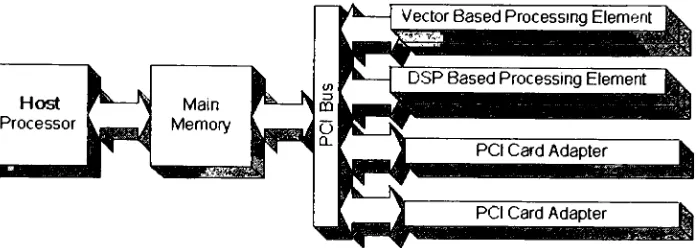
aforementionedlimitations. The
mHC environmentincorporates PCI
based
processing
elements(vector
processors,
digital
signal processors,
etc) into
a general purpose computerthereby
creating
a small-scaleheteroge
neous system wellsuitedto executing
scientific applications.This
environmentis
then
ableto
exploitfine-grained
parallelismby
mapping individual function
calls,
defined
by
the
mHC applicationprogramming interface
(API),
to the
best
suitedprocessing
element
that
is
available.These function
calls arethen
executedin
parallel.Per
formance
is increased
by
running
tasks
onthe
most compatible architecture, whileno
longer
requiring
both
the
high
communication overhead and costs oftraditional
heterogeneous
environments.Through
the
use of a standardAPI,
the
applicationcode
becomes independent
ofthe
microHeterogeneouscomputing
environmentbeing
used.This
greatly increases the
overallflexibility
ofthe
system whilemaintaining
compatibility
withexisting
applications.Furthermore,
the
mHCbased
machines canbe
combinedinto
a clusterusing
suitable
interconnects
which allowsboth
coarse grained andfine
grained parallelismto
be
fully
exploitedto
achieve evenhigher levels
of performance.This
combinationcreates an
extremely
cost effective platformfor utilizing
variouslevels
of parallelismand various architectures
in
orderto
achievethe
highest
performance.A
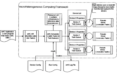
sample mHC environmentis depicted in Fig. 1.1 outlining
these
variouslevels
of parallelism.To demonstrate its
effectiveness, the
framework
requiredto
support mHCbased
large-GrainedParallelism ExploitedByOuster
Sample Apptcation
Clusterof mHCCompfant Computers
Figure
1.1:
A Cluster
of microHeterogeneousComputers
actual applications
to
be
compiled and runusing
standardtechniques.
The framework
consisted of an application
programming
interface
based
on a subset ofthe
GNU
Sci
entific
Library [11],
a real-timedynamic scheduling
algorithm,
and simulateddevices
that
executedthe
variousfunction
calls.Since
real applications were compiled andrun under
the
framework,
accurate performance numbers were obtained andclearly
demonstrate
the
applicability
ofthe
mHC architecture.The
organization ofthe
remainder ofthis
document is
asfollows:
Chapter
2
givessome
background
onheterogeneous
computing,
its
limitations,
programming
andscheduling
methods;
Chapter
3 is
an overview ofthe
microHeterogeneouscomputing
environment;
Chapter
4
discusses
applicationprogramming interfaces
and specifically
ones relevantto
scientificcomputing;
Chapter
5
details
the
microHeterogeneous [image:17.500.90.432.74.306.2]Chapter
2
HETEROGENEOUS COMPUTING
The
concept of microHeterogeneouscomputing is
a variation onthe
standardheterogeneous
computing
environment[14]
[21].
This
chapter gives abrief
background
on
heterogeneous
computersincluding
scheduling
andprogramming
techniques.
The
chapter concludes with adiscussion
onthe
limitations
ofheterogeneous
environments.2.1
Background
Heterogeneous computing is
an architecture which provides an assortment ofhigh
performance machines
for
useby
an application and arosefrom
the
realizationthat
no single machineis
capable ofperforming
alltasks
in
an optimal manner.These
machines
differ
in
both
speed as well asin
capabilities and are connectedusing
high
speed,
high bandwidth intelligent interconnects
that
handle
the
intercommunication
between
each ofthe
machines.Heterogeneous
computing is
an extensionto
homoge
neous
computing,
which usesonly type
ofmachine, that
has
the
potentialto
increase
performance and cost effectiveness.
The
needfor heterogeneous
computers arosefrom
the varying
needs oftoday's
most computation-intensive applications.
These
applicationsgenerally involve
many
different
computing modes,
such asSIMD,
MIMD,
and vectorprocessing,
whichhave
the
potentialto
be
exploited.However,
withtraditional
homogeneous
computersonly
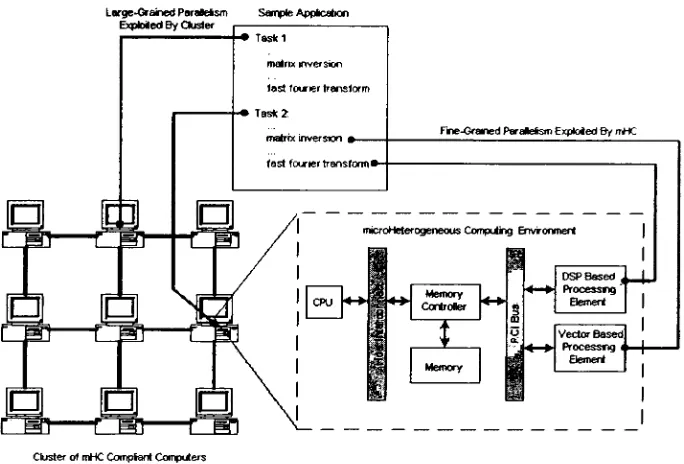
3-Cube MIMO
3x3 Mesh SIMD
3-Cube MIMD
[image:20.500.91.403.73.359.2]Four Element Vector
Figure 2.1: A Heterogeneous Environment
suffer and
thus
limiting
the
effectiveness ofthese
architectures.This is
summarizedby
Amdahl's
Law,
which statesthat the
performance of a systemis
dictated
by
the
percentage of code
that
requires atype
ofprocessing
notparticularly
supportedby
the
hardware.
Heterogeneous
computing
addressesthis
problemby
providing
an assortment ofmachines
that
are capable ofefficiently performing
varioustasks.
Analytical
bench
marking is
usedto
determine
the
optimalspeedup
that
a particular machine canachieve when
it
executes codethat
is
best
suitedfor
that
machinetype.
The
relabasis
ofdetermining
how
well a code segmentis
ableto
be
matchedto the
machine[27].
The
results ofthe
analyticalbenchmarking
arethen
usedto
determine
feasible
partitioning
andmapping
of applications.Once
all ofthe
different
machineshave been
benchmarked,
the
codeto
be
executed must
be
profiled.Since
Heterogeneous
systemsinvolve many different
classes ofhigh
performancemachines,
it
becomes
essentialto
correctly
identify
the type
ofcode
being
run sothat
an attempt canbe
madeto
matchit
withthe
most efficient machine.Without
this
information,
the
performance enhancementsthat
heteroge
neous
computing
environments can provide arelost.
The
profiling
is
done
off-line andis
usedto
determine
the
computing
modethat
exists
in
each program segment aswellasthe
executiontimes.
The different
types that
canbe identified
include:
vectorizabledecomposable,
vectorizablenon-decomposable,
fine/coarse-grain
parallel,
SIMD/MIMD
parallel,
scalar,
and special purpose[15].
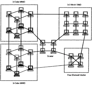
An
example of application
profiling
is
shownin Fig. 2.2.
The
programsegmentsdetermined
by
the
profiler mustthen
be
mappedontothe
most efficient
hardware in
orderto
minimizethe
completiontime
of an applicationrunning
on aheterogeneous
computer.This efficiency depends
heavily
on computation costs,
communicationcosts,
andinterference
costs[22].
Computation
costsinvolve
the
computationtime
of a particulartask
on a particular
machine.Since
aheterogeneous
computerinvolves
many
different
types
ofthe
assigned machine.Communication
costsinvolve
the
communicationtime
between
processors whentasks
aredivided
acrossdifferent
machines and aredependent
uponthe type
ofinter
connectionnetwork used and
the
bandwidth
whichis
available.In
orderto
realizethe
performance
improvements
offeredby
heterogeneous
computing
the
communicationcosts must
be
minimized.The
interconnection
medium mustbe
ableto
providehigh
bandwidth
(multiple
gigabits per second perlink)
at alow
latency. It
must also overcome current
deficiencies
such asthe
high
overheadincurred
during
contextswitches,
the
overheaddue
to the
need ofexecuting
high level
protocols on eachmachine,
andthe
overhead ofmanaging
large
amounts of packets[15].
While
the
use ofLANs
has
become
commonplace, these types
of connections are not well suitedto
heterogeneous
supercomputers.
t
Code Block 1
Code Segment
1
Code Block 2
^
...
Code Segment 2
<' .Code Segment
s a.Rode
Block
n;
mmM
SIMD
MIMD
CO
CO <
Vector
[image:22.500.130.374.419.613.2]Interference
costs
areincurred
when multipletasks
are assignedto
amachine,
which creates resource
contention
and reduces processor utilization.Interference
costsincrease
overall completiontime
andtherefore
must alsobe
minimizedduring
the
mapping.
Mapping
a parallel program onto a parallel architectureto
minimize completiontime
has
already been
shownto
be
anNP-hard
problem evenin
ahomogeneous
environment
[4].
The fact
that
aheterogeneous
computerinvolves
a myriad of machinessimply
complicatesthe
matterfurther. The
efficientmapping,
orscheduling,
ofthe
tasks
of an application onthe
availableresources,
however,
is
one ofthe
key
factors
for achieving high
performance andhas
become
one ofthe
mostintensely
studiedissues
dealing
withheterogeneous computing
environments.2.2
Task
Scheduling
Scheduling
for
aheterogeneous
environmentincludes
of all ofthe
sameissues
found
in
scheduling for homogeneous
environments plussome additionalissues.
Scheduling
needs shared
by
both
homogeneous
andheterogeneous
systemsinclude job
scheduling,
intermediate-level
scheduling,
andlow-level
scheduling.Job scheduling involves
the
selectionbetween
available processesto
run onthe
availablehardware.
The
intermediate-level
scheduling
is in
charge ofsmoothing
operations overfluctuations
in
the
currentload
ofthe
system.The low-level scheduling determines
the
next process
to
run on a machinefor
a certain amount oftime.
The
schedulerin
aheterogeneous
environment must alwaysbe
aware ofthe
dif
most appropriate machine as well as
be
preparedto
reassigntasks
in
casethe
systemconfiguration changes
[15].
In
addition, the
scheduler mustbe
acutely
aware ofthe
bottlenecks
andqueuing delays
causedby
the
heterogeneity
ofthe
hardware.
The
following
are some ofthe
morerecently
developed scheduling
heuristics
in
cluding
Segmented
Min-Min, Max-Min,
andGA. Brief
descriptions
of other commonmapping
heuristics
are also providedfor
completeness.2.2.1
Segmented
Min-Min
In
the
standardMin-Min scheduling
heuristic,
the
minimum completiontime
for
eachtask
is
computed with respectto
each ofthe
machinesthat
arecurrently
present.The
task
withthe
overall minimum completiontime
(taking
any
overheadinto account)
is
selected and assignedto the corresponding
machine.The
task
is
then
removed andthe
process continues until alltasks
have been
scheduled[2,
10].
This heuristic is
very simple,
fast,
and provides good performance.One
drawback,
however,
is
that
small
tasks
are assigned and executedfirst
whichleaves
some machinesidle
whilelarger
tasks
arebeing
executed.The
Segmented
Min-Min heuristic
proposedin
[30]
attempts
to
solvethis
problemby
altering the
Min-Min
algorithmto
schedulelarge
tasks
first.
The
Segmented
Min-Min
algorithmfirst
computesthe
expectedtime to
compute(ETC)
for
eachtask
on eachmachineproducing
anETC
matrix whereETC(i,j)
is
the
ETC for
task
i
on machinej.
The
tasks
arethen
sortedinto
atask
list in
descending
order which
has
the
effect ofpromoting tasks
withlarge
ETC
values.The
task
list is
Segmented
min-min(Smm)
1.
Compute
thesorting
key
for
each task:Sub-Policy
1
Smm-avg:
Compute
the averagevalueof eachrowin
ETC
matrixET<y>
Sub-Policy
2
-Smm-min:
Compute
the
minimum value ofeach rowin
ETC
matrixfcej/i
= minETC(i.j)
j
Sub-Policy
3
-Smm-max:
Compute
the
maximum value of each rowin
ETC
matrixkex/i
=maxETC(i.j)
i
2.
Sort
the tasksinto
a tasklist in
decreasing
orderoftheir
keys.
3.
Partition
the tasks
evenly into N
segments.4.
Schedule
each segmentin
orderby
applying Min-min.
Even
though
Segmented Min-Min only
proposes a slight changeto
the
standardMin-Min
algorithmit
successfully improves
the
load
balancing
and enhancesthe
performance
from
2%
to 12%.
The scheduling
time
is
also reducedbecause
the
Segmented
Min-Min
uses adivide
and conquerstrategy
which reducesthe
search space ofthe
Min-Min
algorithm whendetermining
whichtask to map
[30].
2.2.2
Relative
Cost
Algorithm
The Relative
Cost
Algorithm
uses a relative cost criterion ratherthan
prioritizing
tasks
based
on size.The
relative cost of atask
is
calculatedby dividing
the
task
completion
time
ctk(i,j)
by
the
average completiontime
oftasks i.
This
assuresthat
ahigher priority is
givento tasks that
have
a good matchbetween
tasks
andmachines and minimizes
the
overall completiontime
[29].
The
completeRelative
Cost
RC Algorithm
1.
For
eachtask
i
and machinej,
let ct(i.j)
=ETC(i,j)
andp(i)
=0
ys(iJ)
=ETC(iJ)/ETC(i)avg
2.
For
k
=1
to
t
do
(a)
for
task
i,
1
<i
<t
andp(i)
=0
i.
computectk{i)avg
=^,ij<mctk(i:j)/m
ii.
select machineB,
suchthat
ctk(i,Bi)
=mmi<j<mctk(i,j)
iii.
compute7d(z,
Bt)
=cifc(i,
Bt)/ctk(i)avg
(b)
selecttask
^^
suchthat
-)a{Ak-.BAk)a
x
7d(^c,.4t)
= min-ys(i,B,)a x
7d(z\Bi)
l<t<t,p(i)=0(c)
let p(j4fc)
=1
andF(Ak)
=BAk,
that
is,
assigntask
Ak
to
machineBAk
(d)
for
task
i
with1
<i
<t
andp(i)
=0.
modify
rf,
(,
i)-/
ctk(l'J)
tfJ^BAk
cik+i(i,J)
y
ctk(i.j)
+
ETC(Ak:BAk)
otherwiseThe factor
of7^
x7,,
is
usedto
fine
tune the matching
andload
balancing
criteria.The
smallerthe 7^ the
better
the matching
of machines.Therefore
tasks that
matchmachines
better
willbe
given ahigher
priority.The
a parameteris
usedto
adjust7S,
or
the
static relativecost,
andis
alwaysbetween 0
<
a<
1.
The
specific valuefor
ais generally determined
by
way
of experimentation.In
practice, the
Relative Cost Algorithm
provides a good compromisebetween
load
balancing
andmatching proximity
andconsistently
performsbetter
then
Min-Min,
2.2.3
Heterogeneous-Earliest-Finish-Time
andCritical Path
on aProcessor
Instead
ofusing
a strict performance measurement such as estimated completiontime
or relative
cost,
Heterogeneous-Ealiest-Finish-Time
(HEFT)
andCritical Path
on aProcessor
(CPOP)
determine
task
scheduling based
onthe
application'stask
graph[24].
The
task
graphis
adirected
acyclic graph,denoted
by
G
=(V,E),
whereV
is
the
setOf
vtasks
andE
representsthe
set of e edgesbetween
the tasks.
The
edges represent
the
dependencies between
the
tasks,
with edge(i,j)
meaning
that
task Ui
mustbe
completedbefore
task
nj
may
begin.
Two important
properties ofthe task
graph arethe entry
and exittasks.
Entry
tasks
arethose tasks that
have
noparent
task
and exittasks
arethose tasks
that
have
no children.A
costmatrix,
W,
is
calculatedin
which eachwt j
representsthe
estimated executiontime
oftask
nt
onprocessor
pj
.Tasks
in this
systemare orderedby
their
priorities which arelinked
to
their
upwardand
downward
ranking.The
upward rankis
calculatedrecursively
by
traversing
the
graph upward and
is defined
by
ranku(ni)
=W[
+
max(c7J
+ ranku(nj))
(2.1)
ir,succ(n,)where
succ(ni) is
the
set of successors oftask nz,
is
the
communicationcost of edge(i,j),
andWi
is
the
average computation costfor
task
n{.Therefore,
the resulting
ranku(ni) defines
the
length
ofthe
critical pathfrom
task rii
to the
exittask
andcalculated
by
traversing
the
graph upward andis
defined
by
rankd
(
n,
)
=wl+
max (W~+ cJJ +
rankd(nj))
(2.2)
where
pred(ni) is
the
set of predecessors oftask
n*.The
resulting
rankd(ni) is
the
longest distance from
the entry task to the task rij
but
does
notinclude
the
computation
cost oftask
n,-.The
HEFT
algorithm consists oftwo phases,
aprioritizing
phase and a processorselection phase.
During
the
prioritizing
phase, the task
list is
sortedby decreasing
order of ranku. This provides a
linear ordering
ofthe tasks
which preservesthe
precedence
constraints.Once
the tasks
have been
properly
ordered,
the tasks
are mappedto the
processorsduring
the
processor selectionphase.During
this phase,
an appropriateidle
time
slotis
located for
eachtask.
The
search starts atthe time
equalto the
ready
dime
ofn^
onPj
, orin
other wordsthe time
whenallinput
data
oftask
n^
has
arrived at processorpj
.The
search continues untilfinding
the
first idle
time
slotthat
is
capable ofholding
the
computation cost of
task
nj.HEFT differs
from
mostmapping
algorithmsbecause it
considers
assigning
tasks
in idle
time occurring
between
two previously
scheduledtasks
instead
ofautomatically
beginning
the
searchfor
an appropriate processorstarting
at
the time the
last
scheduledtask
has
completed.The
completeHEFT
algorithmis
HEFT
Algorithm
1.
Set
the
computation costs oftasks
and communication costs of edges with mean values.2.
Compute
ranku
oftasks
by
traversing
graph upward,starting from
theexittask.
3.
Sort
the tasks
in
ascheduling list
by
nonincreasing
order ofranku
values.4.
whilethere
are unscheduledtasks
in
the
list do
(a)
Select
the
first task,
n,from
the
list
for
scheduling.(b)
for
each processorpk
in
the
processor-set(pk
6Q)
do
i.
Compute
EFT(rii,pk)
valueusing
the
insertion-based scheduling
policy.(c)
Assign
task rn to the
processorpj
that
minimizesEFT
oftask
rii.5.
endwhileThe CPOP
algorithm consists of sametwo
main phases asthe
HEFT
algorithm,
a
prioritizing
phase and a processor selection phase.During
the
prioritizing
phasethe
upward anddownward
ranks of all ofthe tasks
are calculated.The
priority
ofthe tasks
is
the
summation ofthe
upward anddownward
ranks.The
critical path ofthe
applicationis
then
determined. First
the entry task
is
selected and marked as atask
ofthe
critical path.The
successor withthe
highest priority is
then
selected andmarked as part of
the
critical path.This
continues untilthe
exittask
is
reached.Once
the
prioritizing
phaseis
complete, the tasks
arethen
mappedto
processorsin
the
heterogeneous
system.Tasks
that
are part ofthe
critical path are mappedto
the
critical-pathprocessor, p^,
which minimizesthe
cumulative computation costs ofthe tasks
onthe
critical path.Tasks
that
are not part ofthe
critical path are assignedto
a processor which minimizesthe
earliest executionfinish
time
ofthe task.
The
CPOP Algorithm
1.
Set
the
computation costs oftasks
and communication costs of edges with mean values.2.
Compute
ranku
oftasks
by
traversing
graphupward,
starting from
the
exittask.
3.
Compute
rankd
oftasks
by
traversing
graphdownward,
starting from
the
entry
task.4.
Compute
priority(rii)
=rankd{rn)
+
ranky(m)
for
eachtask
n,in
the
graph.5.
\CP\
=priority(nentry),
wherenentry
is
the
entry
task.6.
SETqp
=priority(nentry),
whereSETcp
is
the
set oftasks
onthe
critical path.7.
while nkis
notthe
exittask
do
(a)
Select n_,
where((n_,
esucc{nk))
and(priority(rij)
=\CP\)).
(b)
SETcp
=SETCP
U
rij.(c)
nk
<-n,
8.
endwhile9.
Select
the
critical path processor(pep)
whichminimizes_^neS.r
Wi.j.Vpj
Q
10.
Initialize
the
priority
queuewiththe
entry
task.11.
whilethere
is
an unscheduledtask
in
the
priority
queuedo
(a)
Select
the
highest
priority task rii
from priority
queue.(b)
if
rii eSETcp
theni.
Assign
the
task
n, onpep(c)
elsei.
Assign
the task nt to the
processorpj
whichminimizestheEFT(ui,pj).
(d)
Update
the
priority
queue withthe
successors ofnt,
if
they
become ready
tasks.
12.
endwhileWhen
tested
on56,000 randomly
generated
task graphs,
HEFT
andCPOP
onaverage performed
better
then
otherlist
scheduling heuristics
such asDynamic-Level
Scheduling [20], Mapping
Heuristic
[9],
andLevelized-Min Time
[14].
HEFT
producedschedules
that
reduced executiontime
in
86%
ofthe
fifty-six
thousand
randomly
generated
task graphs,
whileCPOP
producedbetter
schedulesin
65%
ofthe
cases.Due
to
the
promising
results andfast
scheduling
times,
HEFT is currently
being
2.2.4
Other
Mapping
Heursitics
Many
othermapping
heurisitics
have been designed
to map tasks
onto aheterogeneous
environment of which
only
a sample aredescribed
here. All
ofthe
following
heuristics
statically
schedule meta-tasks(a
set oftasks
withnodependencies)
ontothe
machines.This
requiresthat
both
the
number oftasks
andthe
number of machinesis
known
before
the
scheduling
processbegins.
All
ofthese
heuristics have
been
evaluatedin
[5].
OLB:
Opportunistic
Load
Balancing
assigns eachtask
in arbitrary
orderto the
first
available machine
[2].
This
technique generally
does
not produce acceptable schedules.UDA: User-Directed
Assignment
assigns eachtask
to the
machinethat
has
the
best
expected execution
time
[2].
This
technique
generally does
not produce acceptable schedules.
Fast Greedy:
Assigns
eachtask to the
machine withthe
minimum completiontime
[2]-Max-Min: A
variationto
Min-Min in
whichthe
task
withthe
overall maximumcompletion
time
from
the
set of all unmappedtasks
is
selected and assignedto
the corresponding
machine[2,
10].
This
technique
generally does
not produceacceptable schedules.
GA: The
genetic algorithm operates on a population of chromosomesfor
a givenproblem and
is
usedto
search alarge
solution space.The initial
populationheuristics
available[26].
This
algorithmgenerally
providesfor
good performancethough
it
is
much slowerthen
Min-Min
whileonly performing
slightly
better.
A*:
A*uses a
tree
based
methodin
orderto
incrementally
build
a solutionfor
the
task
mapping.The
root node ofthe tree
is generally
that
of a nullsolution,
intermediate
nodes represent partialsolutions,
andleaf
nodes representfinal
solutions.
The
nodes are ratedby
a costfunction
andthe
node withthe
minimum
costfunction
is
replacedby
its
children whilethe
node withthe
highest
cost
function
is
removed[7].
This
algorithm providesvery
good schedulesfor
some situations
but is
very slow,
averaging
about1200
times
slowerthen that
of
Min-Min
[5].
2.3
Programming
Parallel programming
environmentsinclude
the tools
neededto
write anddebug
ap
plications
for
parallel machines.These include programming
languages,
compilers,
debuggers
and other aides.A few
ofthe
different
programming
languages
currently
available are
discussed here.
2.3.1
Parallel Virtural
Machines
(PVM)
PVM
(Parallel
Virtual
Machine)
is
a software systemthat
enables a collection ofhet
erogeneous computers
to
be
used as a coherent andflexible
concurrent computationalresource
[18].
The
overall objective ofthe
PVM
systemis
to to
enablesuch a collection
of computersto
be
usedcooperatively
for
concurrent or parallel computation.The
unit of parallelismin
PVM
aretasks
which aregenerally
Unix
processes.communication
and computation.The
systemallows
usersto specify the
set of machines
for
an applicationto
use.The
user alsohas
the
choiceto
viewthese
resourcesas an attributeless collection of virtual
processing
elements or chooseto
exploitthe
capabilities of specific machines
in
the
host
poolby
positioning
certain computationaltasks
onthe
most appropriate computersA
systemlevel
process runs on each ofthe
computer systemsthat
permitsthe
collection of machines
to
be
viewed as a coherent system.The
system supports process
management,
communication via messagepassing,
and synchronizationthrough
the
use of namedbarriers. Important
to
heterogeneous
computing,
PVM
allowsmul-tifaceted
virtual machinesto
be
configured withinthe
sameframework
and permitsmessages
containing
morethan
onedatatype
to
be
exchangedbetween
machineshav
ing
different data
representations.Examples
of programsthat
have
been
executedunder
PVM include
matrixfactorization,
stochastic simulation oftoroid
networks,
and
Mandlebrot image
computations.2.3.2
Message
Passing
Interface
(MPI)
The Message
Passing
Interface
(MPI)
[1]
is
anotherprogramming
environment usedfor
parallelprocessing
andis
compatible withheterogeneous
environments.The
goalof
MPI is
to
create awidely
used standardfor
writing
messagepassing based
applications.
The interface
providedis
practical, portable,
efficient,
andflexible
andhas
become
widely
used.The
implementation
ofMPI is
fundamentally
different
then
PVM. MPI
does
notIn-stead
each processoris
assigned
a rank whichthen
determines
which parts ofthe
application
that
processor will execute.This division
oftasks
among
processorsis
left solely
up to the
developer writing
the
application.The MPI
standardincludes
routinesto
do
point-to-point communicationbetween
two
processing
elements,
collective operationsto
simultaneously
communicateinfor
mation
between
allprocessing
elements,
andimplicit
as well as explicit synchronization.
The
standarddoes
not providedirect
supportfor
sharedmemory
operationsor support
for
threads.
MPI
has
mostrecently
been
usedby
MPEG
encoding
anddecoding
applications[3].
2.4
Limitations
Although heterogeneous
computing
environmentshave
provento
be
very
usefulfor
some
applications,
it
has drawbacks
which preventits
usefrom
becoming
widespread.These limitations include
the
focus
on coarse-grainparallelism, the
inherent
communication
costs,
andthe
actualimplementation
costs.Heterogeneous computing
environmentsfunction
mostefficiently
on applicationsthat
demonstrate
avery
coarse-grained parallelism.This
coarse-grained parallelismresults
in
large
task
sizes and reducedcoupling
which allowsthe
processing
elementsto
work more efficiently.This
requirementis
alsotranslated to
mostheterogeneous
schedulers since
they
arebased
onthe
scheduling
ofmeta-tasks,
i.e.
tasks that
have
no
dependencies.
elimina-tion
[24]
containthis type
ofparallelism, there
aremany
applicationsthat
do
not.These
types
of applicationsmay
have finer-grained
parallelism ortend
to
be
moretightly-coupled
and are not ableto
benefit
as muchfrom
a standardheterogeneous
environment.
In
these
cases,
the task
sizeis
smaller andthe
overhead requiredto
distribute
the tasks
becomes
greaterthen
the
performance enhancement achievedby
executing
the task
on adifferent
architecture.This is
alsotrue
with applicationsthat
include many
dependencies
which require moredata
to
be
passedbetween
machines.The inherent
communication costs are anotherdrawback
ofusing
aheterogeneous
environment.
Generally,
specializedinterconnects
mustbe
usedin
orderto
provide ahigh bandwidth low
latency
connection[15].
These
specializedinterconnects
tend to
be
very
expensive and are not always available.The
other optionis
to
use standardnetworking
equipment(LANs)
whichis
more cost effectivebut
cangreatly hinder
the
overall performance ofthe
heterogeneous
environment.As
the
granularity
ofanap
plication
decreases,
the
performance characteristics ofthe
interconnect
mustincrease
or risk
becoming
abottleneck in
the
system.Finally,
the
implementation
cost ofheterogeneous
networksis
very
prohibitive.Creating
aheterogeneous
network requiresspecialized machines andhigh
speedinter
connectsin
orderto
produce an environment with good performance characteristics.The
cost mightbe
acceptablefor
applicationsthat
areknown
to map
well ontothis
type
ofenvironment,
but in
other casesthey
aresimply
not cost effective.The
next chapterdiscusses
the
roleof application programinterfaces
and specifiChapter
3
APPLICATION PROGRAM INTERFACES
3.1
Background
An
application programinterface
(API),
sometimes referredto
as an application programming
interface,
is
the
interface
by
whichan application program accesses servicesprovided
by
anoperating
system or other applications.An API
provides alevel
ofabstraction
between
the
application andfunctionality
that
the
API
providesto
ensurethe portability
ofthe
code.The
use ofAPIs
in
modern applicationdevelopment is
omnipresent.Computers
have
become
so complexthat
low-level
functionality
is
constantly
being
abstractedto
higher
levels
through the
use ofthese interfaces.
Operating
systems are requiredto
provide one of
the
mostdiverse APIs
that
becomes
the
bridge between
user applications
andthe
hardware
upon whichthey
are executing.Using
anAPI
to
provide accessto underlying
functionality
has
someimportant
benefits. First it
allows an applicationto
maintain portability.As
long
asthe
inter
face
provideddoes
notchange,
an applicationusing
the
API is
notdisrupted
if
the
functionality
that
the
API
providesis
modified.This is
especially true
ofAPIs
that
The
use ofAPIs
also makessoftware
development
easier and more robust.Soft
ware
developers
do
not needto
concernthemselves
withlow-level details
such asdrawing
pixels on ascreen,
sincethese types
ofthings
have
already
been
abstractedto
high level
APIs
such asOpenGL
[19].
APIs
that
have become
a standard are alsowidely
used andtherefore widely
tested,
making the
functionality
that
they
provideless
proneto
errors and moredependable.
For
microHeterogeneouscomputing
environments, the
mostimportant
APIs
arethose
dealing
with scientific computing.3.2
Scientific
Computing
APIs
Heterogeneous
and microHeterogeneouscomputing
aremainly
focused
on scientificbased
applications sincethese types
of programsbenefit
mostfrom heterogeneous
environments.
These APIs
provide accessto the
basic
building
blocks
of scientificcomputing
which canbe
utilizedto
create complete applications.A
few
ofthe
morecommonscientific
computing
APIs
arediscussed here.
3.2.1
Basic
Linear
Algebra Subprograms
(BLAS)
The Basic Linear
Algebra
Subprograms
(BLAS)
[17]
are a set oflow level
operationsthat
arefundamental
to
numericallinear
algebra.The
motivation wasto
create ahighly
optimized set of routines commonto
most scientific applicationsin
orderto
improve
the
overallperformance.Since
a significant amount of executiontime
is
generally
spentin
these
low level
operations, reducing the time
requiredto
performthese
BLAS
is
divided
into
three
separatelevels dependent
onthe type
ofdata
that
is
operated on.The
Level 1
BLAS,
implemented
between
1973
and1977,
includes
subprograms
for
scalar and vector operations.The
software packageLINPACK
usesthe
Level
1
BLAS
extensively for
the
solution ofdense
andbanded linear
equationsand
linear
least
squares problems.The Level 2
BLAS,
implemented
between 1984
and
1986,
deals
with matrix-vector operations andthe
Level 3
BLAS,
implemented
between 1987
and1988,
deals
withmatrix-matrix operations.The linear
algebra software package
LAPACK
utilizesthe
Level 2
and3
BLAS for
portable performance.Overall,
BLAS
have
enabledmany
applicationsto
improve
performance while maintaining
portability.Orginally,
BLAS
wasimplemented in Fortran
66
but
specificationsfor Fortran
77,
Fortran
95,
andC
now exist.Highly
efficient machine-specificimplementations
of
BLAS
are availablefor
almostevery
modern computer architecture.In
general,
BLAS
has been
very
wellreceivedby
developers
for
the
high
performance ofthe
library
routines and
the
portability
that
comes withusing
a standardizedAPI. The
routinesprovided
have
become
the
building
blocks
of alarge
portion of scientific applicationsover
the
pasttwo
decades.
3.2.2
Vector,
Signal,
andImage
Processing Library
(VSIPL)
The
Vector,
Signal,
andImage
Processing Library
(VSIPL)
[13]
wasdesigned
to
provide a
portable,
object-basedAPI for
signal andimage
processing
on embeddedsystems.
The API began development in 1996
by
Hughes Research
Laboratory
andLockheed-Sanders, Nothrup Grumman,
Digital.
Intel,
andCray
withthe
common goalto
createan
industry
supported standardfor
vector and signalprocessing
primatives.One
ofthe technical
goalsthat
VSIPL
setto
achieve wasto
be
very
portable.To
accomplish
this,
the
VSIPL API is implemented
in
ANSI
C
and requiresonly
a simple re-compile
to
portbetween
platforms.The API
alsodoes
not restrictthe
actualimplementation
ofthe
computational portion ofthe
standard.This
allows vendorsto
create optimized
implementations,
if
desired,
whilemaintaining
source-code portability
based
onthe
API.
VSIPL is
an object-basedlibrary,
whichis
adeparture from
traditional
libraries,
such as
BLAS,
that
arefunctional based.
Applications
utilizing
the
VSIPL
API
usespecial abstract
data
types
whoseimplementations
arehidden
to
allowfor
vendor-private
implementations.
The
maindata
types
used areblocks
and views.Blocks
are contiguous storage areas
in
whichthe
actualdata
values are stored.Views
arethen
createdto
determine how
ablock
ofdata is handled. The
three
main view characteristics are offset
from
the
beginning
of ablock,
the
number of elements(length),
and
the
spacing between
the
elements(stride).
For
example,
agroup
of ninedata
elements wouldbe
storedin
a contiguous storage area within a
block
as shownin
Table 3.1(a).
In
orderto
create a viewfor
the
entire
block
as avector, the
offset wouldbe
setzero, the
length
wouldbe
setto nine,
and
the
stride wouldbe
setto
one.If
only the
even elements weredesired,
a viewwould
be
created with an offset ofone,
alength
offour,
and a stride oftwo.
This
123456789
I
2
I
4
I
6
I
8
1
2
3
4
5
6
7
8
9
(a)
A
block
ofdata
(b)
A
view of even elements(c)
A
matrix viewTable
3.1:
Example
ofVSIPL
Blocks
andViews
also
be
used as a3
x3
matrixby
creating
a view with an offset ofzero,
a rowlength
ofthree,
a row stride ofone,
a columnlength
ofthree,
and a column stride ofthree.
This
view would contain all ofthe
data
elementsbut
wouldbe
usedlike
a matrix asshown
in
Table
3.1(c).
The VSIPL
API
supports a wide range offunctions
that
are most commonto
scientific
based
applications
with an emphasis on signal andimage
processing.A
summary
ofthe
functions
included is
located
in
Table 3.2.
VSIPL
alsoincludes
specialaccommodations
for
embedded applications.Better
performance
is
achievedthrough the
use ofearly
binding
which allocates resourcesfor
an operation asearly
as possible.The
memory
spaceis
alsodivided into
a userdata
space and a
VSIPL
data
spacein
orderto
assurethat
data is
not corrupted.The
userdata
space containsdata
the
useris
ableto
manipulatedirectly.
Only
data
in
the
VSIPL
data
space can operated onby
VSIPL
operations andis
hidden from direct
Signal
Processing
Vector/Matrix
Ops
Linear
Algebra
i>FFT >
Convolution
>
Correlation
>
FIR/IIR Filters
>
Arithmetic
>
Comparison
\>
Selection Operations
>
Boolean
Operations
>
Data
Conversion
o
Inner, Outer,
Kronecker
Product
>Matrix-
Vector,
Matrix-Matrix
Multiply
>QR, LU,
Cholesky
Decompositions
t>
Solvers
user manipulation.
In
orderto
makedevelopment
on an embeddeddevice
easier.VSIPL includes
specialdevelopment
modes withhigher degrees
of errorchecking
anda production mode which runs
faster
andincludes
no errorchecking
to
save spacein
embedded
devices.
3.2.3
GNU Scientific
Library
(GSL)
The GNU Scientific
Library
(GSL)
[11]
is
a modern numericallibrary
for C
and C+4-programmers.The
project was startedin 1996
atthe
Los
Alamos
National
Labo
ratory
by
Dr M. Galassi
andDr J. Theiler
afterthey
became
discouraged
withthe
restrictions of
the
licenses
of otherexisting libraries.
With
this in mind,
GSL
wasreleased under
the
GNU General
Public License
(GPL)
[12],
making
the
library freely
available.
With
supportfor
over1000
functions,
GSL
aimsto
providethe
most comprehensive scientific
computing
library
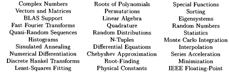
available.A
summary
ofthe
functionality
covered areshown
in
Table 3.3. GSL has been successfully
compiled under all modernoperating
systems
including
SunOS, Solaris,
Linux, HP-UX, IRIX, BSD, Windows,
andApple
Darwin.
GSL
successfully
combines avery
powerfullibrary
with aneasy to
use and understand
interface.
The
library
uses an object-orienteddesign
and allowsdifferent
algorithms
to
be
easily
pluggedin
or changed at run-time withoutthe
needto
recompile
the
actual application.The function
callsfollow
a standardnaming
conventionand
data
types
which makethe
library
particularly
easy for
the
ordinary
scientificComplex Numbers
Roots
ofPolynomials
Special
Functions
Vectors
andMatrices
Permutations
Sorting
BLAS Support
Linear
Algebra
Eigensystems
Fast Fourier
Transforms
Quadrature
Random Numbers
Quasi-Random Sequences
Random Distributions
Statistics
Histograms
N-Tuples
Monte
Carlo Integration
Simulated
Annealing
Differential
Equations
Interpolation
Numerical Differentiation
Chebyshev
Approximation
Series
Acceleration
Discrete
Hankel Transforms
Root-Finding
Minimization
Least-Squares
Fitting
Physical
Constants
IEEE
Floating-Point
Table
3.3:
Summary
ofGSL
Functionality
Another benefit
to the
GSL
is its
compatibility
withother scientificbased APIs. It
provides
direct
supportfor
allthree
levels
ofBLAS,
making
the transition
from
BLAS
to
GSL
atrivial
matter.The
GSL
also usesthe
sameblock
and view representationsof
data
that
VSIPL
uses.This
allowsGSL
function
callsto seamlessly interact
withembedded
devices
based
onthe
![Table 4.2: Comparison of the XP-15 and a 1.4 GHz Intel P4 [23]](https://thumb-us.123doks.com/thumbv2/123dok_us/123638.11982/49.500.44.454.81.204/table-comparison-xp-ghz-intel-p.webp)
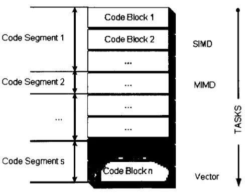
![Figure 4.3: The Pegasus-2 Vector Processing Accelerator Card [6]](https://thumb-us.123doks.com/thumbv2/123dok_us/123638.11982/50.501.82.420.87.263/figure-pegasus-vector-processing-accelerator-card.webp)
![Table 4.3: Pegasus-2 Sample Operation Performance [6]](https://thumb-us.123doks.com/thumbv2/123dok_us/123638.11982/51.500.136.372.82.171/table-pegasus-sample-operation-performance.webp)