A Process Capability Index for Three-Dimensional Data with Circular or Ellipsoidal Tolerances.

Rochester Institute of Technology

RIT Scholar Works

Theses

Thesis/Dissertation Collections

2005

A Process Capability Index for Three-Dimensional

Data with Circular or Ellipsoidal Tolerances.

Veljko Fotak

Follow this and additional works at:

http://scholarworks.rit.edu/theses

This Thesis is brought to you for free and open access by the Thesis/Dissertation Collections at RIT Scholar Works. It has been accepted for inclusion in Theses by an authorized administrator of RIT Scholar Works. For more information, please [email protected].

Recommended Citation

A

Process Capability Index for Three-Dimensional Data with

Circular or Ellipsoidal Tolerances.

Veljko Fotak

December, 2005

A

Thesis Submitted to the Faculty of the Center for Quality and

Applied Statistics in Partial Fulfillment of the Requirements for

the Degree of

MASTER OF SCIENCE in Applied Statistics.

Prof.

Joseph

G. Voelkel

(Thesis advisor)

Prof.

Daniel

R. lawrence

Prof.

Steven Lalonde

Prof.

Illegible Signature

Rochester Institute of Technology Digital Media Library

Electronic Theses, Thesis/Capstone Projects and Dissertations (ETD)

Approval Form

J/,?

If/{

/~r

t?

1<\

Student Name:

_Y_

(L.-_-T) _ _

o

_ _ _

v _ _

v _ _ _ _ _

---,_

Date:

7//Z /05

\;~ (

Degree: __ ~'_~\~=~

____________________ __

r:-College:

t:

V\ U\

l

n

-<2.

e

!'- 'vY\ '\

J )

I

Department/Program:

A(zr

C.J

This is a Master's Thesis

><-.,

Master's Thesis/Capstone Project _ _ or Ph. D. Dissertation (Please check one.)

Title:

A ProcesS

Capo. bi

);.J..

y

TnJex.

~r lTzr~~

-

0;Y12~n5io~/

Qg,±o-

with

Cirw.!ctr c r

EJJiQl50ida.1

To/en::;,oc.

z.::'

5.

I

The above- mentioned thesis, thesis/Capstone project or dissertation has been reviewed and accepted by the student's committee.

Signaturee Date Signed

Joseph G. Voelkel

locI'!

_I

/0;-(Committee Chair)

Daniel

R. lawrence

(Committee Member Co-Chair)

Steven Lalonde

(Committee Member

(Committee Member)

(Committee Member)

Review and Acceptance of ETD: I have reviewed the final electronic version of the above-me[lti(()ned document and determined that it is an accurate representation of the document reviewed' and accepted by th.e committee.

THESIS RELEASE PERMISSION FORM

ROCHESTER INSTITUTE OF TECHNOLOGY

COLLEGE OF ENGINEERING

Title of Thesis:

A Process Capability Index for Three-Dimensional Data with Circular

or Ellipsoidal Tolerances.

I, Veljko F otak, hereby grant permission to the Wallace Memorial

Library of R.I. T. to reproduce my thesis in whole or in part. Any

reproduction should not be for commercial use or profit.

Signature

Velika Fatak

TableofContents

A Process

Capability

Indexfor Three-Dimensional DatawithCircularorEllipsoidal

Tolerances 1

Thesis Release Permission Form 2

Table ofContents 3

TableofFigures 4

Abstract 5

Why

asingle-numerical measure 6

Theproposedprocess_{capability index} 8

Gauge R&R inthree dimensions 1 1

Literaturereview 13

Otherprocess_{capability indices} 15

Calculating

the_summarymeasure of_variability 21

Ageometric interpretationoftheprocedurepresented 24

Estimating

cand_calculatingthemultivariate process _{capability index} 28

Estimating

M 31

Extensions

top

dimensions 32

Application: analysis of color metrics 33

Applications 39

Example 1 42

Example2 51

Example3 57

Appendix 1 64

The function Rub 66

The function Invrub 68

Appendix2 69

The function Pei 71

Appendix3. Dataassumption_checking, instrument

I,

long-term

data,

cyan 73

TableofFJ2ures

Figure 1. Toleranceregionand smallest .99captureellipse 9

Figure2. Tolerance regionand proposed .99capture ellipse 10

Figure 3. Data andtoleranceregion with similarorientations 17

Figure 4. Data andtoleranceregion withdifferentorientations 18

Figure 5. Dataandtoleranceregionwith differentorientations andfittedcapture ellipsoid. 19

Figure 6.

Tolerance,

dataandfittedellipse 25

Figure 7. Transformationto "U-space" 26

Figure 8. Transformationto "V-space" 27

Figure 9. Process capability

indices,

Example 1 46

Figure 10.

Data,

toleranceandfitted ellipsoid,Example 1 48

Figure 11. Tolerance andnatural .99captureellipsoidsforeach var. component,

Example 1 49

Figure 12. Toleranceandfitted .99capture spheresforeach var.component,Example 1.... 50

Figure 13. Process capability

index,

Example 2 53

Figure 14. Data and_{tolerance region,} instrument

A,

Example 2 55

Figure 15. Toleranceregion andfitted.99 capture spheresforeachvariancecomponent,

instrument

A,

Example 2 56

Figure 16. Process capability

indices,

Example 3 61

Figure 17. Dataandtoleranceregion, instrument

A,

Example 3 62

Figure 18.

Tolerance,

.99naturalcapture ellipsoid and.99capturefittedellipsoid, instrument

A,

Example 3 ₆₃

Figure 19. Output ofthePeialgorithm ₇₁

Figure 20. Lightnessversus_time,

long-term,

_cyan,instrument1 74

Figure 21. Chromaversus _time,

long-term,

_{cyan, instrument1 75}

Figure22. Hueversus_time,

long-term,

_cyan, instrument1 76

Figure 23. Normal probabilityplot,

long-term,

cyan, instrument

I,

lightness 78

Figure 24. Normal probabilityplot,

long-term,

cyan, instrument

I,

chroma 79

Figure _{25. Normal probability}plot,

long-term,

_cyan, instrument

I,

hue 80

Abstract

We discuss the estimationof a process _{capability index for} three-dimensional data.

Initially,

we focus onthe case inwhich the _engineeringtoleranceassociated withthe measurements is

a sphere.

Then,

we extend the discussion to the more general case in which the _engineering

tolerance is ellipsoidal. In both _cases, we

develop

_summary measures for repeatability and

reproducibility,to beusedinthe context of a process_{capability index.}

Inthe sphericaltolerance case we_{define summarymeasures,} where each measureis based on

the diameterof a sphere that leads to a pre-specified capture rate (we will usehere 99%). As

a process _capability

index,

we propose _ratios, where each ratio is the diameter of such a

sphere divided

by

thediameterofthetolerancesphere.

In the ellipsoidal tolerance case, such _summary measure will be based on the length ofthe

major axes of the ellipsoid of identical shape and orientation to the tolerance ellipsoid

providing apre-specified capture rate

(again,

we will use here 99%). As aprocess _capability

index,

we propose _ratios, where each ratio is the major axis ofsuch ellipsoid divided

by

the

major axis ofthe toleranceellipsoid.

We present two algorithms in the language R aimed at

facilitating

the estimation of our

summary measure ofvariability. The first algorithm evaluates the _probability that a linear

combination ofthree(or

fewer)

independent chi-square variables willbe lessthanor equal to

a given constant. The second algorithm estimates the value a linear combination of

offer an algorithm in the language R for _computing the process _{capability index in} the

context of color metrics.

Wepresent applicationsto color measurements andto R&Ranalysis of color metrics.

We show how the components of variance in these three-dimensional measurements can be

easily compared to each other and to the tolerance region, using the single-dimensional

summarymeasures of process capability.

Whyasingle-numerical measure

In the single-sample trivariate normal _case, six numbers (three variances and three

covariances) are needed to describe the variability. We suggest here the use of a

single-numerical _summary measure ofvariability, mainly to be used withinthe context of a process

capability

index,

to replacethosesix numbers.

Whilethe use of asingle-dimensionalmeasureof_{variability necessarily leads}to a partial loss

of

information,

there are various advantages of_usingsuch univariate measure:

Such a _summarymeasureallows foran_easy andintuitivecomparison ofthe observed

variability in relation to the defined tolerance region. An appropriate ratio of the

observed _variability to the tolerance offers a meaningful estimate ofthe amount of

tolerance

"used"

Similarly,

such a _summary measure offers an _easy and intuitive comparison ofthe

relative magnitudes of the estimated components of variance

(allowing

for the

identification and comparison of major sources of variation). This measure can then

beusedto prioritize correctiveactions, ifneeded.

A univariate _summary measure allows for other kinds of comparisons of variance

components,

depending

on the particular applications. In the colorimetric example

that we _provide, the univariate measure of _variability offers intuitive means to

compare instruments intermsofthe observed variability.

The proposed measure of _{variability is} easier to comprehend than the six-number

variance-covariancematrix.

Depending

on the _application, other _{summary measures,} or even direct analysis of the

Theproposedprocesscapabilityindex

In the case of spherical _tolerances, we propose to fit a sphere that provides a pre-specified

capture rate to the data. Our proposed process _{capability index} can then be computed as the

ratio between the diameterofthis fitted spheroid and the diameter ofthe tolerance spheroid.

As discussed inthe Otherprocess_{capability indices} section,other metrics derivedfromsuch

sphereshave been proposed inthe past (mostnotably, the volumes),but most methods agree

in

fitting

a sphere _providinga predetermined capture rate.

In the case of ellipsoidal tolerances, as discussed in more detail in the Literature Review

section, it is common practice to base an estimation ofprocess _capability on some measure

relative to the smallest ellipsoid that provides a particular capture rate - for

example,

by

comparingthe lengthofthe major axis of said ellipsoidto the length ofthemajor axis ofthe

tolerance ellipsoid. A two-dimensional representation is available in Figure 1. The smallest

ellipsoid _providing a pre-determined capture rateis what would _{commonly be} usedto derive

[image:11.534.32.431.49.484.2]

Figure 1. Toleranceregion and smallest.99capture ellipse.

Tolerance 99 Data Capture Data

In contrast, we recommend _using a different ellipsoid - that

is,

the ellipsoid with the same

shape and orientation of the tolerance ellipsoid that provides a particular capture rate (we

[image:12.534.24.432.57.533.2]

Figure 2. Toleranceregion and proposed.99capture ellipse.

\

/

/

**V

V

/

,/

Tolerance

99 Fitted Capture Data

We will refer to the smallest fitted ellipsoid (presented in Figure

1)

as "data capture", or

"natural",

ellipsoid and to the fitted ellipsoid ofsame shape and orientation as the tolerance

(as in Figure

2)

as"fittedcapture", or

"fitted"

ellipsoid.

In the case of ellipsoidal tolerances, we propose the use ofthe major axis ofthe ellipsoid of

the same shape and orientation as the tolerance ellipsoid as a _summary measure of

variability.

However,

forthe purposes of a process_capability

index,

the choice of whichaxis

to use leads to invariant results. That

is,

given that the shape ofthe compared ellipsoids is

identical,

the ratio ofthe major axes is identical to the ratio ofthe minor axes

-or, in the

more generalcase,to theratioof_anyother_{corresponding}pair of axes.

Gauge R&R inthreedimensions

We have decided to present the use ofthe proposed _capability indexwithin the context ofa

process _capability, or gauge _{repeatability} and_{reproducibility}

(R&R),

study, as such studies

naturally leadtocomparisonsbetween toleranceregions and variance components.

The simplest R&R scenario involves one _{operator, using} one gauge, _making a series of

measurements on one single part. In the context of an R&R study, the variation of such

measurements can be summarized

by

"repeatability". "Repeatability" is definedas the length

of an interval that captures a predetermined fraction /(we will use_^=

.99) of such

measurements. Inthe case with spherical_tolerance, we estimate _{repeatability}as the length of

the diameter ofthe sphere thatcaptures a predetermined fraction y ofthe reported readings

collected

by

one _{operator,using}one _gauge, onone singlepart.

In R&R studies, it may be possible to further subset _{repeatability into} additive components

labeled "short-term repeatability", "medium-term

repeatability" and

"long

term

If we are to consider a scenario in which one of the above factors (operator or _gauge)

changes, we fall under the realm of "reproducibility".

"Reproducibility"

is defined as the

length of an interval that captures a predetermined fraction y (we will _use/=

.99) of such

measurements. For _example, if we consider multiple operators, using one gauge, each

making a series of measurements on one single _part, we obtain a variation that is

conventionally labeled as "operator reproducibility".

Alternatively,

"reproducibility" can

refer to the case in which we have one operator _using multiple gauges, or

instruments,

to

make a seriesof measurements on one singlepart; inthis case,we speak of"inter-instrument

reproducibility".

In the three-dimensional case with a spherical tolerance, we estimate "operator

reproducibility"

as the length of the diameter of the sphere that captures a predetermined

fraction y ofthe reported readings collected

by

multipleoperators, using one gauge, on one

single part. "Inter-instrument

reproducibility"

will be similarly estimated as the length ofthe

diameter ofthe sphere that captures _y ofthe reported readings collected

by

one _operator,

using multiple _gauges, on one single part

-and so _on, for whatever component of

"reproducibility"

isofinterest.

In the more general case of elliptical _tolerances, we extend the definitions of both

repeatability and_{reproducibility;} that

is,

we estimate_{repeatability} as the length ofthe major

axis ofthe ellipsoid of equal shape and orientation to the tolerance ellipse that captures yof

the reported readings collected

by

one operator, _using one _gauge, on one single part.

"Operator-reproducibility"

canthen_{be similarly defined} asthelength ofthe major axis ofthe

ellipsoid

-of equal shape and orientation to the tolerance ellipse

-that captures_yof the

reported readings collected

by

multiple _{operators,using} onegauge, onone single part.

"Inter-instrument reproducibility"

can then_{be similarly}estimatedas the length ofthe major axis of

the ellipsoid

-of equal shape and orientation to the tolerance ellipse - _that

captures _y ofthe

reported readings collected

by

one _{operator, using} multiple gauges, on one single part

-and

soon, forwhatever component of

"reproducibility"

is ofinterest.

Those components of variance

(repeatability

and _{reproducibility)}

including

possible

interactions (such as, an "operator - _short term"

interaction)

can be estimated _using the

standardMANOVAmethod of moments. Weoffersome examplesinthe

following

sections.

Literaturereview

This thesis extends the work ofVoelkel

(2003),

who examined the two-dimensional R&R

analysis inthe case whenthe specifiedtolerancewas circular.

General

theory

behindgaugeR&Rstudies canbe found in AIAG

(1992),

Wheeler and

Lyday

(1989)

and

Burdick,

Borrorand

Montgomery

(2005).

The application presentedhere is relatedto color metrics. Volz

(1995)

discusses multivariate

analysis of color metrics.

The process described falls under the wider _category of"coverage problems", discussed

by

Guenther andTerragno (1964).

The estimation of our _summary measure of _variability requires the estimation of the

probability that a non-negative linear combination ofindependent chi-square variables will

be smallerthan or equal to a given constant. The same distribution of quadratic

forms,

with

relative _application, has been discussed in various different contexts.

Johnson,

Kotz and

Balakrishnan

(1998)

offer an extensivediscussionofthe_existing literatureon the topic.

The distribution of a linear combination of j2

random variables, in particular, has been

discussed andtabulated

by

Grad and Solomon

(1955),

by

Solomon

(1960)

and

by

Marsiglia

(1960)

in the bi-and tri-variate cases. Johnson and Kotz

(1968)

presented tables for 4 and 5

dimensions and Solomon and Stephens

(1977)

offered tablesbased on linear combinationof

6,

8 and 10 variables.

The ideas proposed

by

Solomon were developed into a series ofalgorithms; in particular,

Sheil and O'Muircheartaigh

(1977)

offer an algorithm (AS

106)

to calculate the _probability

thata linearcombination ofA'non-central independent x~

random variables willbe less than

or equal to a constant c. Davies

(1980)

offers an algorithm (AS

155)

with the same

functionality,

but employs inversion of the characteristic function to obtain _{the solution,}

basedon a _previouslypublished paper

by

the same author (Davis (1973)). Farebrother

(1984)

offers an improved version (AS

204)

to the algorithm AS

106,

leading

to _{generally faster}

computing times. The algorithms AS 155 andAS 204 are both based on a method outlined

by

Ruben (1962).

Johnson,

Kotz andBalakrishnan

(1998)

discussother approaches thathave

been employed to estimate the distribution function of a linear combination of chi-square

variables.

Otherprocess_{capability indices.}

Voelkel

(2003)

discussessome _summarymeasures of_variabilitythathave been considered in

the past. The discussion is specific to the case in two

dimensions,

but the concepts _apply

similarlyto our case.

Inparticular, the area of an ellipse of equal shape and orientation to the tolerance ellipsehas

been proposed

by

Hulting

(1992). We believe this _summary measure of_variability to have

one major

difficulty

in interpretation. While this area-based measure is mathematically

equivalent to the circle-diameter _measure, in most applications the users are more often

thinking

interms of original units ofmeasure, ratherthen in terms ofthe squared _{(or cubed)}

units associated with tolerance surfaces and volumes. The sphere-diameter measure that we

propose is expressed in the original units ofthe measurements, thus _offering more intuitive

interpretations.

The length ofthe major axis ofthe natural ellipse _providing a specific capture rate

(Hulting

(1992)

and Demeter

(1989))

has some appeal as it is a _{very intuitive summary} measure of

variability. We discuss here why we consider it an _{ineffective summary}measure to be used

withinthe context of aprocess_capability index.

When the defined tolerance is spherical, there is no difference between the length of the

diameter of the "natural" sphere _providing a certain capture rate and the length of the diameter ofthe fitted sphere _providing the same capture rate, as the two will be necessarily

equivalent. Ontheother

hand,

with an ellipsoidal tolerance,a comparison ofthelength ofthe

majoraxis ofthe ellipsoid_offeringa specific capture rate _{could, potentially,} offer_misleading

results.

We will illustrate the _possibility of_misleading results in two dimensions. Consider a

two-dimensional dataset with its smallest, or_natural, .99 data capture ellipsoid. Assume that the

size and shape of said ellipsoid are _very similar to the size and shape of the tolerance

ellipsoid.

If,

for _{example, the} direction of maximum _variability of the data was _perfectly

aligned with the direction of maximum _variability ofthe tolerance region, as in Figure

3,

a

ratio ofthe major axis ofthe data and tolerance ellipses close to 1 would appear to suggest

that the observed _variability is about the same size of the tolerance region,

leading

to an

acceptable product, or process. The dataset depicted includes 100 data points. As expected,

given a capturerate of.99, we can observethatone pointfallsoutside of our .99datacapture

ellipsoidandoutsidethe toleranceregion.

Please note, a ratio larger than 1 would indicate that the proportion of observations

falling

withinthe tolerance is smallerthan thepredetermined capture rate (.99). A ratio smallerthan

1 wouldindicate that theproportionofobservations

falling

withinthe tolerance is largerthan

the predetermined capture rate (.99). A process _{capability index} smaller than 1 is thus

desirable.

[image:19.534.17.447.42.510.2]

Figure 3. Dataandtoleranceregionwithsimilarorientations.

^

+

\ S_

r*

*l^fi^

-Tolerance

-.99 Data Capture

+ _Data

T

If,

on the other _{side, the} direction of maximum _variability ofthe data was not aligned with

the tolerance region, as in Figure

4,

_anyratio basedon a comparison oflengths or surfaces of

the two depicted ellipses would still be approximately

1,

but the number of observations

falling

outside ofthe tolerance region would be considerably higher. In our example, only

one observation falls outside ofthe .99 capture ellipsoid, but 7 observations fall outside the

tolerance region.

Clearly,

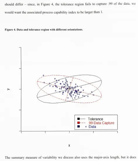
theprocess _{capability indices for}thecases in Figure 3 and Figure 4

should differ

-since, in Figure

4,

the tolerance region fails to capture .99 of the

data,

we [image:20.534.29.501.49.600.2]

would want theassociated process_{capability index} tobe largerthan 1.

Figure 4. Dataandtoleranceregion withdifferentorientations.

+ 7^

' ----t +-fcT V

-i

\

/

X

/+

K

X

'l

.

J^

-Tolerance

-.99Data Capture

+ _Data

T

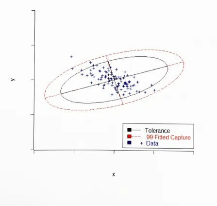
The summary measure of_variability we discuss also uses the major-axis length, but it does

account for the differences in orientation between the data and tolerance region, thus

being

preferred in most applications. Given the same scenario as the one presented in Figure 4,

when _computing a process _capability

index,

we would fit the capture ellipse presented in

Figure 5. The ratio ofthe length ofthe major axis of said ellipse to the length ofthe major

axis of the tolerance ellipse _{is approximately 1.3}

-indicating, correctly, that the process

variability is indeed larger than the tolerance region. In this example, the predetermined

capture rate is .99, but the tolerance region only captures 93% of the

data;

with out

methodology, the associated process _{capability index is correctly} estimated as

being

larger [image:21.534.26.473.303.727.2]

than one.

Figure 5. Dataandtoleranceregion withdifferentorientations and fittedcapture ellipsoid.

.<T^, s

1

/

/

r

-Tolerance

-.99

Fitted Capture

+

Data

Wang

et al.

(2000)

discuss three other multivariate process _{capability indices (we} cite the

relevantindices inthree-dimensional_{applications,} although allthreehave beenpresented ina

more generalmultivariatesetting):

Shahriari,

Hubele and Lawrence

(1995)

propose a _{capability index based} on three

components: a ratio of volumes (the numerator

being

the volume defined

by

the

engineering tolerance region and the denominator

being

the volume of a modified

process region

-the smallest region similar in shape to the _engineering tolerance

region, circumscribed around a_probability contour), a measure ofthe distance ofthe

centers ofthe tolerance and dataregions and an indexvariable

indicating

whetherthe

modifiedprocessregion isoris not contained withinthe tolerance regions.

Taaam,

Subbaiah and

Liddy (1993)

propose a _{capability index based} on the ratio of

thevolume ofthe toleranceregionto thevolumeof a modified process region

(which,

inthe caseofmultivariatenormal

data,

is an ellipsoid_providing a99% capturerate).

Chen

(1994)

proposes a _capability index to be applied, as the title of his paper

suggests, to rectangulartoleranceregions. His index has no intuitive interpretation in

themultivariate _case,but it isexpressedintheoriginal unitsofmeasure ofthedata.

Kotz and Johnson

(2002)

present an extensive list of publications _regarding process

capability

indices,

andlisttheavailableliterature on multivariateindices.

Calculating

thesummarymeasureof variability

Consider the simplest case of one operator, using one _{gauge, making} a series of

measurementson one single_part, inwhichwe wantto estimate repeatability.

We assume that the variation in these measurements can be modeled

by

a multivariate

(trivariate)

normal

distribution,

_which, without loss of _generality, we assume is centered at

zero:

x~n3(o,i:s).

We also assume that the given toleranceregion is atri-dimensional ellipsoid

(or,

in a special

case, a _sphere) centered at zero. An ellipsoid can be _{mathematically} described

by:

{x

: x'Mx= c2

),

where M is a non-negative definite symmetric matrix

defining

the shape of the ellipsoid and c is a scale factor. For the tolerance ellipsoid, we set c- 1

, which

reduces the equation ofthe tolerance ellipsoid to

{x

: x'Mx=l}. The _{tolerance region can}

thenbe describedas theseries of points

{x

: x'Mx <

1}

.

Please note _that, forthe present purposes, an ellipsoidal and aspherical tolerance region are

treatedinthe same manner.

In orderto compute our _summarymeasure of_variability, we aim at

fitting

an ellipsoidwith

the same shapeandorientationas those of_{the tolerance ellipsoid,} sothata certainproportion

(the "capture_rate") ofthe observeddata falls withintheellipse

itself;

that

is,

we wanttofind

c suchthat:

P(X'M

X<c2)

=

In geometric _terms, we wantto shrinkorstretch the tolerance matrix M

by

a factora so that

wefindthematrix ofthe same shape and orientationthatgives:

P(X'aMX

<l)=y

_or, equivalently:

P(X'aMX<l)=P X'MX <

-= PJX'MX< c2

)

= y

V

a) Where c2 =l/a

In order to more _{easily find c,} we can equate the quadratic form X'MXto a linear

combination of independent chi-square variables (as the distribution ofthe latter has been

amply discussed in the past in the context of "coverage problems", as discussed in the

Literature reviewsection ofthe present). Toaccomplish this goal, we _apply a series ofthree

transformations of variables. While these three transformations could have been

accomplished in a _single, albeit more _{complex, transformation,} we present them here in a

step-by-step fashiontofacilitate understanding.

As afirst_step,we set U =_MI/2X .

U is a lineartransformation of a multivariate normal random _variable; it is well know that U

itselfis also multivariate normal:

U~N3(0,i:u)

, where

u

= Ml/2i:xMl/2.

Because X'MX =X'Ml/2Mi/2X = U'U

, p(x'MX < c2

)=

p(u'U <c2

)

Eu

is a symmetric positive definite matrix and can be decomposed as follows (Johnson and

Wichern

(2002,

pp. 66-67)):

u

=

PuDuP,;

where

Du

isadiagonalmatrix_containingthe eigenvaluesof

Hu

:

D.

K

o o

o

zU2

0

0 0 I

Where

Xu_

_,/lUi and

Xlh

aretheeigenvalues ofthematrix

u

and

Xu_

>

Xu^

>

Xih

and

Pu

=[eU|

,eU2,euJcontains the corresponding orthonormal eigenvectors; we should

note that P.'

P..

=1.

Ina second_{transformation,} weset V =

P^

U.

Thevariance-covariancematrix ofV is:

ln=p:eupu=p:pudup;pu=idui =

du

Thatis,V~N3(0,Du).

Wethen

finally

havetheequation:U'U = VT^P^'V = V'V

.

Sincewearehere

discussing

the_{tri-variate case,}

X'MX = U'U=VV = V2

+V; +

V2

Since

V],V2

and

VJ

are normal variables with _{variance, respectively,}

Xu

,XlH and/lu , we can

equate: V2

+V22 +

V^

=

Xu

Y2 +_/LH Y2 +

Xu

732, where

Yx

,

Y2

and

Yi

are independent standard

normalrandom variables.

That

is,

we have equated X'MX to a weighted sum of independent chi-square _variables,

each with one degree of

freedom,

where the weights are the eigenvalues of the

matrix

u

=

M1/2LXMI/2 :

p(x'MX<c2

)

= P(U'U <_c 2

)

= P(v2 + V2 + V2 <c2

)

=

p(XUi

Y;

+

Xu^

Y; +

^

Y2 <c2

)

=

y

After

briefly

discussing

the _geometry ofthe above transformations, we will discuss how the

proposed process _{capability index} reducesto c.

Ageometricinterpretation_oftheprocedure presented

We havepresentedthe aboveas three consecutivesteps inorderto _{simplify understanding} of

theprocedure. Thethree steps takencan be easilyexplained when looked at _sequentially and

with a geometrical interpretation. Figure

6,

Figure 7 and Figure

8,

on the

following

pages,

offera graphical representation ofthe process.

Please _note, we have assumed _previously that our measurements follow a multivariate

normal

distribution,

centered at_{zero; that}

is,

X ~

N3

(0,

x

)

.

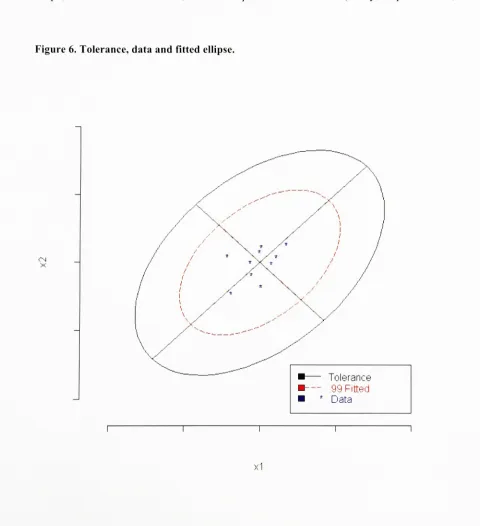
Step

1: Please refer to Figure 6. _{Our starting} point is the equation of the tolerance

ellipsoid, which we can describe

by

a sequence of points

{x

: x'Mx=

lj

. A second ellipsoid,

with the same shape and orientation, provides a predetermined capture rate and can be

described

by

the set of random variables

(X

:X'MX <

c2

}.

Thetwo ellipsoids have the same [image:27.534.9.489.185.711.2]

shape,orientationand _{centroid; the two}ellipsoids differ in scale(set

by

the parameter c).

Figure 6._Tolerance, dataandfitted ellipse.

CM X

-Tolerance

-99 Fitted

*

Data

x1

Step

2: Please referto Figure 7. The firsttransformation,U= M1/2X

, hasthe effect of

shrinking both the tolerance and data ellipsoids _along the directions of maximum _variability

(axes ofthe tolerance ellipsoid). Both ellipsoids reduce to spheroids; the tolerance ellipsoid

can be described

by

a set ofpoints

{u

: u'u=

l},

_whilethe fitted _{ellipsoid can} be described

by

a set of random variables

(U

: U'U <c2

Figure 7. Transformationto "U-space".

CM

Tcrerance 99 Fitted

Data

u1

Step

3: Please refer to Figure 8. The second transformation,V = _P^U

, rotates both

the tolerance and fitted regions. The resulting spheroids have their axis aligned with the

coordinate systems. Both ellipsoids reduce to _spheroids; the tolerance ellipsoid can be

described

by

a set ofpoints

{v

: v'v _=1), while the fittedellipsoid can be described

by

aset of

random variables

[V

: V'V< c2

Figure8. Transformationto "V-space".

>

Tolerance 99 Fitted

Data

i

v1

[image:29.534.10.468.23.715.2]

Estimating

c and_calculatingthemultivariateprocess _{capability index.}

As discussed in the literature review _section, various methods and algorithms have been

proposedinthepastto solve:

P\XU

Y2 +

X:i

Y2

+

Xu

732

<c2)=

y,where

7,, 7,

and

Y}

are independent standard normal

random variables.

In Appendix 1 we use two algorithms to solve the above equation. The first estimates

ygiven the eigenvalues

Xu

,

Xu

and

Xu

and the parameter

c2

; the second algorithms

estimates

c2

given theeigenvalues

Xu

,XU^ and/lu andtheparameter y.

The

inequality

_\r\P\Xu Y2

+

Xu

Y2 +

Xu

Y2 <c2

)=

_{y is} overparametrized. An often used

reparametrization employed, for example, in the tables compiled

by

Marsiglia

(1960),

leads

to: P(Y2+r]Y2+r2Y2 _<r3) =

y

Where

'

i

=

K

IK

r2 =

\

IK

r^c2jXUi

We will continue to use the overparametrized version of the equation in the present

discussion.

Once we have M and c, we can proceed _{in estimating} our _summary measure of_variability

and _computing the _{capability index} as follows.

Geometrically,

as discussed

by

Johnson and

Wichem

(2002,

pp.

65-66),

the three-dimensional fitted ellipsoid can be determined

by

the

three axes, whose orientation is described

by

the eigenvectors _etofthe matrix M and whose

half length inthe _e(direction is equalto , where

Xt

isthe

/"'

correspondingeigenvalue

ofthematrix M.

Inthe spherical case, wehave

Xx

=

X2

=

X3

= X

. The diameterofthe spherecanbe calculated

as d=

2c/

Jx

.

For the purposes of _calculating the _capability

index,

we calculate the diameter of the

tolerance sphere:

dlol

- 2 1

-[X

Theprocess _capability

index,

definedas the ratiobetween the diameter ofthe "fitted" sphere

andthe diameterofthe tolerancesphere, reduces to:

d

_

2c/

VI

d,o,

~

2/

VI

=_c

In the ellipsoidal _case, wecalculate the lengthofthe major axis ofthe ellipsoid, ofthe same

shape and orientation as the toleranceellipsoidthatprovides apre-determinedcapture rate_/.

Our process _{capability index} will then be the ratio ofthe major axis ofthis ellipsoid to the

major axis of the tolerance ellipsoid.

Clearly,

for the purposes of

developing

a process

capability

index,

theratio ofthemajor axes will be equalto the ratio of e.g. the minor axes,

becausethe shapesofthe ellipsoidsareidentical.

The length of the major axis of the fitted ellipsoid will be equal to

2c/^Xmin

where

Xmm

=

min(/l1,

X2

,

A3

)

. Please note, that the major axis ofthe ellipse isassociated with

the smallest eigenvalues ofthe matrix M

-as the length of each axis is

inversely

related to

the size ofthe eigenvalues ofM. The length ofthe major axes ofthe tolerance ellipsoid will

be equalto:

2/^jXmm

, sotheprocess capability index

is,

again, c.

Theprocess _capability

index,

defined asthe ratio betweenthe length ofthe majoraxis ofthe

"fitted"

spheroid andthe lengthofthe major axis ofthe tolerance ellipsoid,reduces to

2c/y/C

2/V-C

The use of c as a scale factor allows for quick and intuitive comparisons.

So,

for _example,

ifc=0.1

, we would conclude that the amount oftolerance

"used"

by

the data

-or

by

the

particular variance component studied - is 10

percent. This also allows for comparisons of

variance components.

Estimating

M

In some _{applications,} the users _may not be given a matrix M that describes the size and

orientation ofthe tolerance region.

Rather,

a set ofacceptableobservations _{may be}provided,

from which the user has to derive an equation

describing

the tolerance region. A similar

approach was used in the field of color science to derive a series of equations

describing

tolerance regions whose size and orientation _{vary according}to the position in color space of

the measured sample.

We define

t;

asthe vector oflength 3 containingthe measurements ofthe

i'h

observations.

Ifwe consider a set ofdata points

describing

the entire acceptable tolerance region, define

tol

asthesample variance-covariance matrix associated withthis set ofdatapoints.

Wethenproceed

by finding

thevalue _c]calej =

t-S^t,

for everyobservation /.

We_{define c]cale}

,max

=

max(c2.afe,

)

. We thendefine M as:M

=

1^,

.

scale, max

Extensionstopdimensions

We presentour methodin _{the three-dimensional case,} but the argument applies _equally well

to thep-dimensional case.

With spherical _tolerances, our_summarymeasure wouldbe the diameterofthe p-dimensional

spheroidthatleadsto apre-determinedcapture rate.

With ellipsoidal _tolerances, our _summary measure would be the length ofthe majoraxis of

the ellipsoid (ofequal shape and orientation to the tolerance _ellipsoid) that leads to a pre

determined capture rate.

When

fitting

this ellipsoid,we would use a similar set of equations:

p(x'MX<c2)=p(uV<c2)=P(J^XUpY2<c2).>

p

p

With eitherspherical or ellipsoidal _tolerances, c can be interpreted as _estimating the fraction

oftolerance "used"

by

the component of variance ofinterest.

In practice, the main use of this is in the two-dimensional _{case, extending} the result of

Voelkel (2003).

Application:analysisofcolor metrics

We present in the

following

section various applications ofthe proposed process _capability

index,

in the context of color metrics. Our process _capability index is presented within the

framework ofthe

CIE94

(Bems

(2002,

pp.

72-74))

standard for color measurements. In the

present _section, we

briefly

summarize the most relevant

CIE94

concepts andhow

they

reflect

onthe applicationof our process _{capability index.}

Onecommon coordinate systemfor reportingcolor

data,

andthe format inwhichthe datasets

weremade available to us, isthe CIELAB coordinate system (Bems (2002),pp. 72).

Briefly,

CIELAB can be described as a rectangular coordinate system with axes labeled L ,a and/? .

Themagnitude ofthe

L*

coordinate describestheamount of

lightness,

that of refersto the

amount of redness-greenness while that of b*

refers to the amount of yellowness-blueness.

"CIE"

stands for Commission Internationale de l'Eclairages

-an international

body

of color

scientists -while

"LAB"

refersto the L\ and b*

coordinate system.

Every

measurementcan

thenbe

described,

withinthe CIELABmeasurement_system,

by

a vector v =

[L*

bj.

Despite the common use ofCIELAB in reporting

data,

CIE94

definescolor tolerances within

a different coordinate _system, defined _simply as

"lightness-chroma-hue",

with axes

labeled

L\

C*ab,

H'ah.

CIE94

offers an equation to estimate the size of the acceptable tolerance region for color

differences (Berns (2002, pg. 72). While this above equation was developed to estimate the

size of a tolerance region around a particular

"standard",

we have applied a slight

modification to the formulas supplied, in order to compute color differences around the

mean. Wedefine:

A94

= ^=1 f *^* V + AC_ab \kcSc j AH V ab \^h^hj , where:

Sc

= ₁₊

0.045CJ,

S

=1+

0.015^

kL

-kH

-kc

= ₁for_{reference conditions}

Similarly,

with slight modifications to the standard formulas (Berns

(2002,

pp.

72),

Stokes

(1992),

Seve(

1996)):

M!=L'balch-T

*c:b4aijAbijf4d*r+(b>)f

AH h = ab ala,c,y -a'bla,ch

[0-5(C,to,cAC

+ +b'ba,chb

* )f2

Finally,

to obtain an estimate of our tolerance _region, given a certain position in the

.

b'

color space, which reflects in the

C*ab

factor,

we have to set a maximum acceptable

"overall color

difference",

asmeasured

byAf94

. Forthepurposes ofthe presentexample, we

will _setA94 -

1,

a value

commonly used in industrial application, although the exact value

will depend on the particular application studied. In an applied situation, the value of

AE94

willbe established

by

theuser.

Theregion _containingacceptable observationcanthenbe describedas:

T:

'AT

V K^L^LJ ( K^* \ ab AC \kcScj f A IT* V AH_ab ykf/Sfj _j <1

Given a set of Z,*,a*and

b*

measurements, we are then able to both transform the data and

derivean equationforthe toleranceregionin

AL*

,

AC*fc

,

AH*ah

space.

Thesizeandorientation ofthetolerance region canbe described

by

adiagonalmatrix:

M =

0 0

1

^

0

0 _A2

1/

We should observe that the tolerance ellipsoid axes defined

by

the

CIE94

_standard, are

aligned with the

AL*

,

AC*ab

,

AH*ab

coordinate system.

To estimate the scale factor c for a particular variance _component, we need to estimate the

eigenvaluesofthematrix

Eu

=

MI/2LXM1//2

, which inturnrequires anestimateof

x

.

In our simplest scenario (one operator, using one gauge to take n measurements on a part),

we could model each_reading

Xx

=

AC*ab AH*ah

)

as follows:

X;

=

p+>,with:

p =

(0

₀

ei~N3(0,LJ

We can_easily estimate

Hx

as

Var(AX*

)

Cov(AC;A,AI*)

CovfA/CAT)

Cov(az.*,ac;J

Var(AC;J

Cov(AH*ab,AC:b)

Cov(AL*.AHlb)

'

cov(ac;,a//;J

Var(A^;J

Once we have obtained our estimate of xas described above, we can proceed

by

finding u

=M'/22:xM

1/2y- M\/2

We then calculate the eigenvalues

X,

,X, ,X, of the matrix and use the latter in

estimating cin P[X

Y2

+

Xu.

Yi

+

K,

Yi

^c2)=y.

To find c for a given set of eigenvalues

Xu

,

AUi

,

AM

and a capmre rate /, we proposed an

algorithm in Appendix

1,

which is an adaptation of the Ruben algorithm presented

by

Farebrother(1984).

In more complex cases, such as a typical gauge R&R study, we are interested in the

estimation of components of variance. In typical applications, we can assume that the

variation of a process can be subset into _short, medium and

long

term components. For

example,we couldassume thatwe couldmodel each_{reading xijk} =

\AL*ijk

ACa/,

AHabj as

follows:

xjik = _u+

si

+mj

+'k' with:

u=

(0

0

s, ~MVN(0,Ls)

i^-MVISKO.EJ

lk

~MVN(0,L,)

Please note that the total error term xis equal to the sum of the short, medium and

long

termcomponents:

Xx

=

Es

+

Em

+

,

.

Multivariate ANOVA _{techniques and,} in _{particular, the} so called "method of

moments"

(Montgomery

(2001,

pp

512-549),

Jobson (1999),

Rencher(2002))

can be employed to

obtain

Es,Hm

and

,

. Wecanthencalculate:

tu-s

u,m=M'/2i:mM1/2

tUJ

=

M1/2L,M1/2

'/2V lVfl/2

u

=Ml/-ExM

Wecan thenobtainthe foursets of eigenvaluesto obtain estimates of_c,csl,cml,ch.

These fourestimates would correspond to common summaries ofthemeasurement systems.

Forexample, cslwouldbe anestimateof shorttermrepeatability.

In the one-dimensional _case, we can observe

that:c2

=

c],

+c2ml

+cft. Voelkel

(2003)

proved

that, in the two-dimensional case,

c2

<c2

+_c2ml

+cft

-the case for perfect _{additivity only}

holds when all ofthe components of variance are oriented in the same direction (that

is,

the

estimated variance-covariance matrices all have the same eigenvectors). The same concept

appliesto three ormore dimensions:

c2

<c2

+_c2, +

c,2

, withtheequality

holding

only when

all components ofvariancehave thesamespatial orientation.

In the same _way the method of moments applied to univariate cases can result in negative

component of variance _estimates, in multivariate settings the method ofmoments can result

inestimatedmatricesthatarenot non-negative definite.

From our _examples, we observed that this problem tends to most often manifest

itself,

in

multivariate_settings, whenmost ofthe variance is alignedwith onedimension. For_example,

we encounteredthisproblem when _estimatingvariance componentsin ourthird example (the

long-termcyandata).

When the estimated components of variance arenot non-negative definitematrices, we used

the Calvin-Dykstra algorithm(CalvinandDykstra (1991)). Otherpossible remedial measures

aredescribed

by

CalvinandDykstra(1991).

Applications

We present here three different examples, all relative to estimation of variance (and

components of_variance) of color metrics.

1. An estimation of

inter-_{instrument reproducibility and of the related components of}

variance (short terms and medium

term)

and possible interactions

(instrument*

medium-term), basedon measurements on awhite sample.

2. A comparison of the components of variance (short-term and _medium-term) of

measurements obtained with 12 different

instruments,

based on measurements on a

white sample.

3. A comparison of the long-term and medium-term _variability components of 12

instruments usedtomeasure acyantile.

The instruments used in the three examples are ofthree different kinds: handheld spheres,

benchtop

spheres andhandheld bidirectional. The instruments were labeledasfollows:

Table 1. Instrumenttypes.

Instrument Type

A Handheld Sphere

B Handheld Sphere

C Handheld Sphere

D Handheld Sphere

E

Benchtop

Sphere

F

Benchtop

Sphere

G

Benchtop

Sphere

H

Benchtop

Sphere

I Handheld Bidirectional

J Handheld Bidirectional

K Handheld Bidirectional

L Handheld Bidirectional

Twopairs ofidenticalmodels wereincluded inthe experiment: Aand

B,

Kand L.

The experiments were conducted under the assumption that no operator effects would be

significant. Under this assumption, no data on operators has been collected and the

assumption itselfcouldnotbe tested.

The capturerate _{y for}the data-fittedellipsoidshas beenset in theseexamples at .99.

The data was made available to us in the L metrics. We converted to

AL*

,

AC*lh

,

AH*ab

spaceusingthe formulas discussed inthe previous section.

After converting the data to

AL*

,

AC*ab

,AH

*ab

space, we proceeded

by

verifying that the data

did meet our assumptions

-that

is,

that the data is multivariate normal and that no trends

over time are present. Our technique requires also that the mean of each univariate

distribution is zero

-given that

AX*

,

AC*,,

,AH

*ab

are essentially differences from the mean

value,

they

are_necessarilycentered at zero.

We first checked for independence over time (that

is,

for a lack of time-related trends or

measurement drift). No formal tests were employed

-rather, the data was plottedversus the

order of observationand_{visually inspected for}trends.

In order to _verify the _normality assumption, we utilized four univariate tests

(Shapiro-Wilkins (Shapiro and Wilkins

(1965)), Kolgomorov-Smirnov,

Cramer andAnderson

Darling

(Ryan and Joiner

(1976)))

to check for departures from normality in the univariate data

distributions.

Finally,

we employed the Mardia tests for Skeweness and Kurtosis (Mardia

(1980))

and the Henze Zirkler T-test _{for normality (Henze} and Zirkler

(1990))

to check for

multivariate departures. We used normal _probability plots and chi-square

Q-Q

plots

(Chambers, Cleveland,

Kleiner and

Tukey

(1983))

to assess univariate and multivariate

normality departures. The procedureappliedis exemplifiedforone instrument in Appendix 3.

Overall,

we were satisfied with the results of such tests and concluded that the data did not

presentproblematic departures fromourassumptions.

Example 1

The dataset used in this first example consisted of 10 measurements taken _every

hour,

for 8

hours,

on each of12 instruments.

We assumethatwe couldmodel each_{reading xijk} =

\AL*jk

AC*ab

AH*ah

J

as follows:

Xijk

=_M-+

mi +

ij

+

miij

+

Sk(ij)

> with:

u=

(0

0

m1~N3(0,LII1)

1,-^(0,2.)

mi^-N^O,^)

sk(ij>

~

N3

(0,

Es

)

, where wedefine:

Hx

=_{total variance}

Ls

=_short-term (within_the

hour)

variance component

m

=_medium-term

(hour-to-hour)

variance component

Lj

=instrument_{variance component}

Emi

=instrument

-mediumterminteractioncomponent

Using

the

CIE94

equations, we find that the tolerance matrix associated with a white sample

is_simply asphere:

M =

1 0

0 1 0

0 0 1

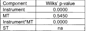
We report here one ofthe metrics used in the test for significance ofvariance _components,

the p-valueassociated with the F statistic for

Wilks'

multivariate test (Johnson and Wichern

(2002)). When tested at a 5% significance

level,

the instrument and the instrument-medium

term interaction components of variance were _significant, but the medium-term component

was not. In our_analysis,we retainedthe MT componentof_variance,because thehigher-level interaction is significant; in order to obtain a meaningful estimate of

Lm

, we applied the [image:45.533.41.224.290.356.2]

Calvin Dykstra algorithm).

Table 2.Significanceof variance_{components, Example 1.}

Component Wilks'

p-value

Instrument 0.0000

MT 0.5450

lnstrument*MT 0.0000

ST na

Using

the expected mean square table presented in Table 1, we obtainedthe

following

estimates for

ourcomponents of variance:

2.

=

^.3289

.0261

.0261 .0541 -.0234

.0077 -.0234 .0257 v

^.0425

-.0010

-.0010 .0006 -.0001

.0019 -.0001 .0006

mi

=

^

.1225 .0096 .0005

A

.0096 .0037 .0005

.0005 .0005 .0005

J

=

f

.0054 -.0005 .0003^

.0005 .0000 .0000

v .0003 .0000 .0000

:

= 1

.1585 .0179

.0179 .0498 -.0238

.0050 -.0238 .0246

Table3. EMS for Example 1.

Source df EMS

Instrument 11 L,+10Elm+80E.

MT 7

Ls+10Emi+120i:ni

lnstrument*MT 77

^s+102mi

ST 864

^s

Total 959

Once we obtained the above estimates, we could _employ the algorithms presented in

Appendix 1 to calculate our process _{capability index for} each component of variance.

Keeping

in mind_that,because M = I ,

E

=M1/2t

M1/2 =

t

iu,st=M|/2i:stMl/2=i:st

E =M' E M' =E

u,instrument*mt instrument*mt in:strument*mt

t,

u,mtmt mt =i\,mtm,

rV2 _ = MV . M' = E. u.rnstrumentt instrumentt rnstrumentt

The estimated process _{capability indices for}each component of variance and forthe total are

presented in Table 4 and plotted in Figure 9.

Table 4. Process capabilityindices,Example 1.

Component

c~

c

Instrument 1.17 1.08

MT 0.04 0.19

InsfMT 0.82 0.91

ST 0.28 0.53

Total 2.29 1.51

Figure_{9. Process capability}indices,Example 1.

o

Tolerance

o

Inst MT InsfMT

Component

ST Total

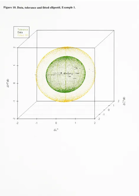
[image:48.534.9.498.35.684.2]

Figure 10 depictsthe data _{points, the tolerance}region and the .99 capture region ofthe same

shape and orientation as the tolerance region. In this case, as the c value of 1.54

indicates,

the length ofthe major axis ofthis fitted region _{is approximately 1.5} times the length ofthe

majoraxis ofthe toleranceregion.

Figure 1 1 depicts the tolerance region and the natural .99 capture ellipsoids relative to each

variancecomponent.

Figure 12 depicts the tolerance region and the fitted spheres relative to each variance

component. As the c value of 1.08

indicates,

the instrument-to-instrument component of

variance

by

itselfexceedsthe size ofthe toleranceregion.

Figure10.Data,toleranceandfittedellipsoid, Example 1.

/

TO X <

^^^a^^^jgg

i

o

AL1

_Cl

"

U

[image:50.534.32.503.37.701.2]

[image:51.534.10.452.43.698.2]

Figure 11. Toleranceand natural.99capture ellipsoidsforeachvariancecomponent,Example1.

Tolerance

99 MT

99InsfMT

99 ST

_d

CD

X <

I

0

AL*

-> *

"

O

<

f -1

[image:52.534.15.516.36.694.2]

Figure 12. Toleranceandfitted.99capture spheres foreachvariancecomponent,Example 1.

X

To 1era net

99 MT

99InsfMT

99 ST

-2 0

AL*

ro

o <1

Example 2

The dataset used in the first and second example consisted of 10 measurements taken _every

hour,

for 8

hours,

on each of12 instruments. Inthe secondexample, we conductedaseparate

analysisforeach ofthe 12instruments.

Because the sample measured is the same white _tile, the tolerance matrix is the same

employedin Example 1:

M

1 0

0 1 0

0 0 1

For a given

instrument,

we assume that we could model each _reading

X,

=

(Ai;

AC;^ A//;a

)'

asfollows:

Xu

=M-+si(j)+mj,with:

p =

(0

0

si(j)~MVN(0,Es)

mj~MVN(0,i:m)

We allowfor

Ls

and

Lm

tobeestimated _{separately for}eachinstrument.

We testedforthe significance of variance components and obtained estimates forthe sumof

square and cross product matrices associated witheach variance component. Basedonthe

p-value associated withthe F statistic for

Wilks'

multivariate _test, all ofthe tested components

[image:54.533.42.226.208.301.2]

of variance were significantat a5%significance level.

Table 5.EMS,Example 2.

Source df EMS

MT 7

2.+10E.,

ST 72

m

Total 79

When computing these components-of-variance _estimates, we obtained s matrices as components

estimates that were not non-negative definite. We employed the Calvin-Dykstra algorithm to obtain

newestimatesforthosecomponents.

Our_results,presented in Table 6 andFigure

13,

point to dramatic differences inperformance

across instruments. Instruments

C, D,

K andL obtained c values larger than _one,

indicating

that a portion of their observations is expected to fall outside of the tolerance region. In

instruments C and D this was due to a large medium-term variance component. A similar

phenomenon was observed for instruments K and

L,

but here the short-term component of

variance appears_{considerably larger}thanforotherinstruments aswell.

Table6. Process capabilityindices,Example2.

Instrument ST

7

c

MT Total ST

c

MT Total

A 0.0006 0.0301 0.0305 0.0237 0.1734 0.1747

B 0.0005 0.0761 0.0766 0.0233 0.2758 0.2767

C 0.0624 1.3390 1.4000 0.2499 1.1572 1.1832

D _j 0.0211 3.5563 3.5777 0.1454 1.8858 1.8915

E 0.0051 0.0251 0.0302 0.0715 0.1583 0.1737

F 0.0001 0.0006 0.0007 0.0121 0.0239 0.0263

G 0.0001 0.0003 0.0003 0.0073 0.0170 0.0178

H 0.0003 0.0024 0.0026 0.0175 0.0488 0.0511

1 0.2004 0.0955 0.2946 0.4477 0.3090 0.5428

J 0.0400 0.5281 0.5643 0.1999 0.7267 0.7512

I K 1.2742 0.8451 2.1176 1.1288 0.9193 1.4552

L 1.8503 4.0083 5.8074 1.3603 2.0021 2.4098

Figure 13. Process capabilityindex,Example 2.

CO CD CN lO CD d Tolerance

mtttiW

m _ST ? MT ? Total

j_n

B D E F G H

Instrument

K

[image:55.534.10.468.52.705.2]

We can also use the concepts presented here to estimate the proportion of points expected to

fall within the tolerance region, for each variance component. We do this

by

_solving

P[XU

y2

+

Xuy2

+

Xu

_v3 < l)= _{y for y using thefunction Rub}presentedin Appendix 1.

The expected proportion of observations within tolerance relative to each variance

component foreach instrument is presented in Table 6.

Table 7. Expectedproportion of observation _fallingwithintolerance, Example 2.

Instrument ST

r

MT Total

A -100.0% -100.0% -100.0%

B -100.0% -100.0% -100.0%

C -100.0% 97.4% 96.8%

D -100.0% 82.8% 82.6%

E -100.0% -100.0% -100.0%

F -100.0% -100.0% -100.0% G -100.0% -100.0% -100.0%

H -100.0% -100.0% -100.0%

1 -100.0% -100.0% -100.0%

J -100.0% -100.0% 99.9%

K 97.8% 99.5% 92.3%

L 94.2% 80.1% 71.1%

As an example, we presentthe results obtained for instrument A in Figure 14 and Figure 15.

Figure 14 presents the data points and the tolerance region. Figure 15 depicts the tolerance

region andthe fitted spheresrelativeto each variancecomponent.

Figure14.Dataandtoleranceregion,instrument_A,Example2.

[image:57.534.13.453.49.565.2]

Figure 15.Toleranceregion andfitted.99capture spheresforeach variance_component,instrument

A, Example2.

X <

..-j^rt^^^rsy-s^ /

ro

6

<

[image:58.534.13.483.54.691.2]

Example3

The datasetusedin thisexample included 12 instruments (labeled A-L), each usedto make2

measurements _every

day,

for 25

days,

on a cyan sample. Data for Instrument D was _missing

for 3

days,

data for instrument E was _{missing for 5 days} and data for instrument H was

missing foroneday.

Weconducteda separate analysis foreach ofthe 12 instruments. We assume_{that, for}a given

instrument,

we could model each_reading X,, =

\AL*

,

AC*h

AH*h

I as follows:

Xu

=M-+

mi(j)

+1^1111:

p=

(0

0

lj~N3(0,Ek)

Becasewe are_measuring adifferent samplethan the white usedinthe firsttwo examples,we

haveto usethe

CIE94

equationstodeterminethe size and orientation ofthe toleranceregion.

To obtain the equation of the tolerance matrix, we calculated a *

andb

*

and the related

parameters, obtainingtheresults presented in Table 8.

[image:60.534.27.500.47.463.2]

Table 8. Toleranceregionparameters, cyan,Example 3.

Parameter Value

meana*

-28.3605

mean b* -38.4245

meanC*ab 47.7573

l/S/2

1.0000

l/Sc2

3.1491

l/Sh2

1.7164

The resultingtoleranceregion can then be described

by

thematrix

M

1 0 0

0 3.14 0

0 0 1.72

We tested forthe significance of variance components and obtained estimates forthe sum of

square and cross product matrices associated with each variance component. We used the

p-value associated with the F statistic for Wilks' multivariate test to determine which

components of variance were not significant; we set the level of significance at 5%. All of

the components of variance tested resulted _{statistically} significant, except for the

Using

the expected mean squares presented in Table

9,

we obtained estimates for the

variance-covariance matrices associated with each component of variance, for each

instrument.

When computing these components-of-variance estimates, we obtained some matrices as

components estimates that were not non-negative definite

(namely,

the estimates ofthe

long

term variance-covariance matrices associated with instruments

B,

F,

J,

K and L). We

employedthe Calvin-Dykstraalgorithmtoobtain newestimates forthosecomponents.

Using

the algorithm presented in Appendix

1,

we were then able to compute our process

capability indicesas shown in Table 10 andin Figure 16.

Table9._EMS,Example3.

Source Df*

EMS

LT 24

E.+2L,

MT 25

m

Total 49

Table 10. Process capabilityindices.Example3.

Instrument MT

2

C

LT Total MT

c

LT Total

A 0.1087 0.0000 0.1087 0.3296 0.0000 0.3296

B 0.0603 0.0797 0.1399 0.2456 0.2824 0.3741

C 0.1054 0.0000 0.1054 0.3246 0.0000 0.3246

D 3.4117 0.0000 3.4117 1.8487 0.0000 1.8487

E 0.1930 0.0522 0.2445 0.4393 0.2285 0.4945

F 0.0234 0.0185 0.0411 0.1531 0.1359 0.2028

G 0.0088 0.0450 0.0534 0.0937 0.2120 0.2312

H 0.0026 0.0286 0.0311 0.0508 0.1690 0.1763

1 0.1006 0.0212 0.1134 0.3172 0.1455 0.3367

J 0.1329 0.0852 0.2170 0.3645 0.2920 0.4659

K 0.1117 0.0903 0.2017 ] 0.3342 0.3006 0.4491

L 0.2582 0.0270 0.2683 0.5081 0.1642 0.5180

Allofthe instrumentsexceptfor instrument D

display

_{repeatability}well withintolerance.

Themediumtermvariancecomponent of_D, with an associated c value of

1.8,

isthe_only

component of variance _exceedingtolerance.

[image:63.534.16.485.33.557.2]

Figure 16. Process capabilityindices,Example 3.

o

LO

CN

O

CM

Tolerance

IMlfl

LjueUIM

ABCDEFGH I J K L

Instrument

Figure 17 is a plot ofthe dataandtolerance region. Figure 18 depictsthe results obtainedfor

instrument A. As the LT variance component resulted non _significant, the ST variance

component isequalto the totalvariance.

[image:64.534.22.479.36.690.2]

Figure 17. Dataandtolerance region,instrumentA,Example 3.

ro

X

-3

ro

3 f

<

0

AL1

[image:65.534.30.503.49.696.2]

Figure 18._Tolerance,.99natural capture ellipsoid and

.99capturefittedellipsoid, instrumentA,

Example 3.

Toleran 99 Data 99 Fitted

CO

X <

_Q

ro

u <

AL*

Appendix 1

The algorithm is an iterative search _procedure, used in _solving

P(XlY]"

+

X2Y2

+/l3F32

<

c2)=

y for c, given the eigenvalues_/I,,

X-,

,

X3

and the desired probability /, where

Y,

,

Y2

,

73

are independent standard normal random variables. The

algorithmis inthelanguage R.

The core of the search procedure is a function named Rub (after Ruben

(1962));

the

algorithmis basedon

AS204,

by

Farebrother

(1984),

which inturns employs Ruben's

(1962)

method to evaluate the _probability that a linear combination of n non-central chi-square varia