A Layer-Based Data Model as a Basis for Structuring 3D Geometrical Built-Environment Data with Poorly-Specified heights, in a GIS Context

City, University of London Institutional Repository

Citation

:

Slingsby, A. (2007). A Layer-Based Data Model as a Basis for Structuring 3D

Geometrical Built-Environment Data with Poorly-Specified heights, in a GIS Context. Paper

presented at the 10th AGILE International Conference on Geographic Information Science,

Apr 2007, Aalborg, Denmark.

This is the unspecified version of the paper.

This version of the publication may differ from the final published

version.

Permanent repository link:

http://openaccess.city.ac.uk/565/

Link to published version

:

Copyright and reuse:

City Research Online aims to make research

outputs of City, University of London available to a wider audience.

Copyright and Moral Rights remain with the author(s) and/or copyright

holders. URLs from City Research Online may be freely distributed and

linked to.

A Layer-Based Data Model as a Basis for Structuring

3D Geometrical Built-Environment Data with

Poorly-Specified heights, in a GIS Context

Aidan Slingsby

The giCentre, Department of Information Science, City University, London, UK

INTRODUCTION

Vector geometrical information systems1 (GIS) can be used to hold, display, process and analyse map-based geographical information (geometry and attributes) for a variety of applications. This paper will concentrate on those associated with the built-environment. Whilst most other geometrical modelling software types handle true 3D information, commercial GIS software remains underdeveloped in this regard. There are a number of reasons for this, one of which is the motivation for this work – that complete and structured 3D data of the built environment is difficult to obtain, for which good 2D data already exist. Unstructured 3D point cloud datasets (for example, obtained from LiDAR) are widely used to augment 2D data in GIS, however, these are unsuitable for gathering data on underground spaces, spaces hidden from above by overhead detail and spaces within buildings. 3D built-environment data can be obtained from architects and engineers, but there are barriers to its use

in terms of detail of detail, semantics and georeferencing (van Oosterom et al, 2006). The use of

standards such as the Industry Foundation Classes in architecture (Eastman, 1999; Liebich 2003) and the emerging CityGML standard for virtual cities (Kolbe, 2003) are helping to address these problems.

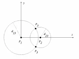
Figure 1: There are two possible positions for point P3, which is constrained to distance d13 from point P1 and distance d23 from point P2 (Chen et al., 2007).

The majority of the geometrical models proposed for use in 3D GIS (e.g. Molenaar, 1990; Pilouk, 1996; Zlatanova, 2000) and 3D geoinformation exchange standards (OGC, 2002) are coordinate-based boundary-representation models. However, they require fully-specified data for their population. In this paper, a system is proposed, based on the concept of constraint-based modelling for managing the combination of 2D data with incomplete height data. Constraint-based modelling is ordinarily associated with design, allowing design constraints to be specific, such that solvers can automatically suggest solutions. They are applied widely (computer aided design, graphics, user interfaces) and many types of algorithms solving constraint-based design problems have been developed (Hower and Graf, 1996). In the building construction industry, constraints can specify the

1

geometrical and topological arrangements of rooms, early examples of which are OXSYS CAD, CEDAR and HARNESS (Eastman, 1999). Geometrical solvers allow geometrical problems layouts to be constrained through positional, angular and topological constraints (Chen et al, 2007); see figure 1 for an example. Here, it is proposed that the constraint-based modelling approach can be used manage incomplete data, by representing them as constraints to a 3D geometrical problem.

The proposed model comprises complete 2D data arranged into topologically-connected surfaces. These are annotated with an incomplete set of ‘height constraints’ representing measurements (including spot heights, specified vertical separations between layers and surface discontinuities), which constrain the 3D form, effectively ‘pinning down’ positions within layers. From these, a 3D geometrical solution can be generated, whose quality is dependent on the input data and how well the constraints constrain the 3D form of the surfaces. Further height constraints can subsequently be added, in order to improve the quality of the model. The fact that only measurements are stored (as constraints) requires a potentially computationally-intensive process of resolving a 3D geometry, but it also offers opportunities for quantifying uncertainty in the 3D output. The system proposed is intended purely for data storage and management, with the output is intended for use in GIS or other analysis packages.

It is hoped that models based on this approach can allow height data to be better exploited, and that the generated 3D geometries, can be applied to a similar range of uses to those of large scale digital mapping data. The surface-based topological structuring makes the proposed model a suitable candidate for pedestrian modelling applications over multiple storeys of the built environment. Additionally, 3D datasets of buildings can be potentially used for analysing statistics relating to buildings, their uses and their inhabitants, especially in multiple-occupancy buildings (Steadman et al, 2000).

REPRESENTATION

Topologically-connected layers

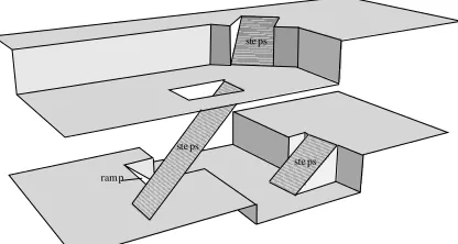
The model – which is based on Slingsby (2006) and Slingsby et al (2007) – abstracts the built

environment (including building interiors) into a series of topologically-connected layers, as shown in Figure 2, comprising of a topological set of points, lines and polygons. Layers represent the ground surface on which human activity takes place and the topological connections between layers correspond to human access between layers, which are stored as a seamless multilayered set. It is thus limited in representing the 2D footprints of those spaces in which human activity takes place and connectivity of these spaces.

ste ps ste ps

ste ps ramp

Types of height constraint

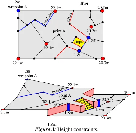
The height constraints are annotated versions of the 2D geometrical primitives which comprise the layers, which are illustrated in Figure 3. In the prototype, there are two types of positional constraint (‘absolute heights’ and ‘relative heights’), two types of linear constraint (‘breaklines’ and ‘offsets’) and two areal constraints (‘ramps’ and ‘stairs’).

20.3m 1.8m

1.8m 1.8m

1.8m 1.8m steps

20.3m

20.3m 20.3m

20.3m 20.3m

offset

off set

22.1m

offset

breaklin e

22.1m 22.1m

22.1m

22.1m 22.1m 2m

wrt point A

2m wrt point A

point A

point A

brea klin

e

Figure 3: Height constraints.

The positional constraints are based on 2D point primitives. An ‘absolute height’ acts as a spot height – a 3D coordinate which pins the layer down at a particular 3D position (six of which can be seen in figure 3). ‘Relative heights’ enforce a vertical separation between two positions, either both on the same surface or different surfaces. They can be used in two contexts, either along an ‘offset’ to specify the height at the particular position (in Figure 3, two enforce a 1.8m vertical separation along an offset), or as a spot height whose height is described with reference to another (in Figure 3, the reference geometry is labelled as ‘point A’). The latter context can also be used to enforce a separated between layers, for example for the height of a bridge. Figure 4 shows the effect of the reference geometry on the resulting 3D geometry.

Absolute height Absolute height Absolute height _{Absolute height}

Absolute height Absolute height

Re lative height

relative to A

Relative height

with no relative geome try assigne d

Relative height

relative to B

A

A

A

B

B

B

Linear constraints are based on 2D line primitives and they specify characteristics of the surface morphology. ‘Offsets’ specify that there is vertical separation between the polygons on either side of them, by an unspecified amount; this information is supplied by strategically-placed relative heights as shown in the previous paragraph. The amount of vertical separation may vary along an offset edge, as can be seen by those on either side of steps. ‘Breaklines’ are breaks of slope.

Areal constraints are based on 2D polygon primitives. ‘Ramps’ are used to indicate that the area is inclined (sloping) and that the surface should be horizontal in the direction of movement. ‘Stairs’ similar, but they indicate that the surface is stepped

Since it is likely that the system will be very under-constrained, a set of rules are required to assist in the generation of a 3D solution. Due to the prominence of horizontal surfaces in the built environment, it is assumed that all surfaces are horizontal, in the absence of constraints to the contrary.

Data input specification

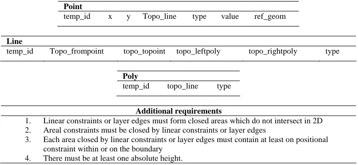
Figure 5 shows the specification of the input data expected by the prototype, as a topologically-connected set of point, lines and polygons. The topological information is given by the attribute preceeded with ‘topo’ (there are equally valid alternative ways in which the topological information can be expressed). Each geometrical element has ‘temp_id’ which must be unique in the set of geometries imported so that geometries can be referred to. If the geometry is a constraint, the constraint type is placed in the ‘type’ field. Point constraints have a height value (either an absolute or relative height); ‘ref_geom’ is the geometry from which the relative height value is with respect to. The algorithm also requires the additional requirements listed in Figure 5 to be met. The reason for these will become clear in the next section. Additional geometries can be added and existing geometries modified (e.g. modifying a point to an absolute height) in order to improve the model.

Point

temp_id x y Topo_line type value ref_geom

Line

temp_id Topo_frompoint topo_topoint topo_leftpoly topo_rightpoly type

Poly

temp_id topo_line type

Additional requirements

1. Linear constraints or layer edges must form closed areas which do not intersect in 2D 2. Areal constraints must be closed by linear constraints or layer edges

3. Each area closed by linear constraints or layer edges must contain at least on positional constraint within or on the boundary

4. There must be at least one absolute height.

Figure 5: Input data specification.

THE ALGORITHM

The algorithm operates locally on units called ‘patches’. A patch is a set of topologically-connected geometrical primitives whose resulting surface is continuous; i.e. is differentiable at every point. They are automatically and transparently identified from the layers by using linear constraints, assuming the input data are specified as in Figure 5 (the first two ‘additional requirements’ must be met). Figure 6 shows how the multilayered set is split into 4 patches.

ramp

absolute height (23.2m)

relative he ight (-0.6) w.r.t. upper geometry

off set edge

relative height (4.5) w.r.t. polygon A

23.2m

polygon A

offset br eakline

A

B

C D

Figure 6: Automatic identification of 4 patches.

Patches are not stored persistently, but are delineated when required to encompass at least all the geometries for which a 3D output is required. The algorithm then attempts to build a surface for each patch as a triangular irregular network (TIN). This process is not straightforward for two reasons. Firstly, patches have height dependencies on each other (due to ‘relative heights’). If a patch’s height is dependent on another, which in turn has its height dependent on another, the problem becomes very complicated. Secondly, height constraints may be under- or over-specified (Chen et al, 2007). If the latter two ‘additional requirements’ (Figure 5) are met, the data will never be too underspecified for a solution to be produced, because all patches will have at least one height constraint and, as stated earlier, they will be assumed to be horizontal in the absence of other information. This is shown in Figures 7 and 8 (note however, that these have multiple solutions which are arbitrarily chosen).

z=? z=?

z=? z=?

z=23.4 z=23.4

z=27.5 z=20. 1

z=23.4 z=23.4 z=23. 4 z=23. 4 z=23.4 z=20. 1 z=23.4 z=20. 1

Figure 7: Allocating heights to vertices with unknown heights – assumption of horizontality.

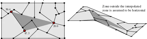
50.4

47. 3

20.0

Z one which can be interpolated

Z one outside the interpolated zone is assumed to be horizontal

The complications which arise from interpatch dependency mean that TINs cannot necessarily be built in one go without building the TINs of dependent patches along the way. Thus, TINs are built incrementally, often in several iterations until all the height constraints have been satisfied. The height constraints used for building TINs are classified into three groups, in order of priority of addition:

1. all absolute heights and those relative heights whose heights are not dependent on the TIN

of any other patch (they lie completely within one patch);

2. relative heights whose height is dependent on the TIN of another patch and the coordinates

of breaklines (which act as relative heights of zero);

3. relative heights between patches whose height is with reference to the patch being built

The prototype was implemented in Java, and Figure 9 describes the getTin() method of the ‘Patch’ class. The first constraints added are those which are not dependent on other patches. Where constraints are dependent on other patches, the getTin() method of the dependent patch is called recursively. If it is the first time it is called on that patch for that constraint and if the TIN is incomplete (each patch keeps track of the remaining constraints it has to add), it continues building the dependent patch’s TIN. It then returns either a fully-resolved TIN (which may involve yet further recursive getTin() calls) or its incomplete TIN.

call t o 'getTin' method

call t o 'getTin' method

[yes] [succes s] [no] [yes] [no] [no] [fa ilure] [yes] has the TIN been

res olved?

List 1: add the geometries one-by-one

List 2: add the geometries one-by-one

List 3: add the geometries one-by-one

Store current state of TIN

Check T IN is fully resolved

dependent on another TI N? for each

try to calculate height has Patch been visited already?

add geometry to TIN

re move geometry from list

Instance of 'Patch' _{Instance of the}

depend ent 'Patch'

Instance of 'Tin'

I nstance of 'Tin' belonging to th is patch

F ind and sort the cons traints of this patch into 3 lists:

1)

2)

3)

abso lute and relative h eights, complete ly within the p atch, with no dep endent patches

relat ive heights whose reference heigh t is with reference to a geomet ry in a different p atch

relat ive heights whose reference heigh t is with reference to a geomet ry in the same patch

Use stored T IN

Calculate TIN

Use ( incomplete) existing TIN, to avoid endless loops Recurs ively

calcula te TIN

Can do so, if the TI N has at least one node with a height

Be cause it's been added successf ully

Returns a TIN

TIN is fully resolved if List 1 and L ist 2 are empty (because the contents have bee n added). Conte nts of list 3 are only added by this patch if additions from the first two lists fail - other wise they a re dealt with by the adjacent patch.

*

relative he ight

relative height

relative he ight

relative height relative he ight

abs olute height

A

Trying to re solving the height here

Figure 10: Dependent patches: to resolve the height marked with an asterisk, the majority of these patches must be resolved because of the position of the only absolute height.

Figure 10 illustrates the recursive nature of the algorithm. If the TIN of the patch marked with the asterisk is required, the dependent patches and their dependent patches need to be resolved in order to find the absolute height marked ‘A’, before any of the TINs of the intervening patches can be resolved. Areal constraints (ramps and stairs) form their own patches, and the surface geometry is constructed using other techniques.

The algorithm works incrementally, gradually building the TINs, constraint by constraint, repeating until either all the constraints have been used (in under- or well specified cases) or until a cycle has passed with no further constraints added (overspecified cases). It finds the first, rather than optimal solution. The solution it arrives at is dependent of the order in which the patches are visiting and the order in which the constraints are added. This is discussed further in the following section.

EVALUATION

Examples

Figure 11 shows a complicated arrangement of connected ramps and staircases, which was built using the data specification and algorithm described above. Only one absolute height was given. Note the use of the offset line for the kerb.

underground passage sta irs

ramp

stairs stairs

stairs

road

kerb

space underneath building

door flush with terrain (which als o gives the split storey its height) door flush with ter rain

(which also gives the split storey its height)

door flush with terrain

offset edge

offset edge offset edge

offset edge gap in wall

height of offset and steps purely dependent

on the heights of the terrain at e ither door

this line is not topologically connected to the input laye r 0

Figure 12: Buildings on a hillside.

Figure 12 is a more complicated example depicting a group of buildings on a hillside, which has a number of interesting characteristics. The hillside geometry is due to a number of absolute heights. The only height constraints of the two buildings on the left are relative heights of zero with respect to the hillside at the entrance doors. The floors of the building are horizontal, because no other height data has been specified; this is according to the rules applied by the algorithm. The height difference between the two floors in the split-level building on the left is entirely due to the hillside heights outside the entrance doors. The offset between the split level cause these to be on different patches. Since there is no height constraint along this offset, these two patches are disconnected in the sense that there are not dependent on each other for their heights. The building on the right has a sloping floor. Its heights are a relative height of zero at the entrance and a relative height at the back of the building, with reference to a point on the hillside. This forces a vertical distance separation between the hillside and the floor of the building.

Quantifying uncertainty

The fact that the model is designed to do its ‘best’ with incomplete data, inevitably results in different degrees of certainty at different positions. However, by assessing the distribution and density of constraints, it is possible to quantify the level of uncertainly in the resulting 3D geometry (assuming constraints are certain). This is an issue for further work.

Height constraint conflicts

Multiple 3D solutions and sensitivity of processing order

As stated, the resulting 3D geometry may be dependent on the order in which the height constraints and patches are processed. This is the case where incomplete TINs have been used and where patches have been assumed to be horizontal in order to resolve relative heights. Since the algorithms terminates when a solution has been reached, no information is provided about the number of alternative solutions. In order to obtain all alternative solutions with the algorithm described here, it would have to be run for every possible order of constraints and patches. However, details of what was done and assumed at each step of the algorithm run may provide an indication of possible alternative solutions.

Computational efficiency

Where there are few absolute heights, the number of dependent patches on any one patch may be very high. In Figure 10, in order to even begin building the surface geometry of the asterisked patch, a patch with an absolute height must be sought, built and then all the patches between. Additionally, trying the prioritised list of height constraints, failing and trying more in the meantime is very computationally intensive.

Although it is likely that the algorithm implementation can be improved, these problems listed above arise from the complexity of problems which the system is designed to deal with.

CONCLUSION

In the context of the development of coordinate-based 3D GIS data models, the increasing demand for 3D data of the built environments, the difficulty in obtaining height information and the good availability of 2D data of the built environment, this paper outlines a system for managing a set of incomplete height data (it does, however, require fully-specified 2D data). The system uses a series of height constraints embedded in ground- or floor-based 2D data, using layer topology and various rules and assumptions to store the geometry of the built environment, from which a 3D geometry can be generated when needed.

The algorithm for generating the 3D geometry from the 2D data and the set of height constraints is described. Examples of its use are given and its characteristics and weaknesses are identified and discussed. These weaknesses, however, are mainly due to the ability to deal with poorly-resolved data, though, the implementation can certainly be modified to run be made to be more efficiently.

This work aims to explore an alternative approach to 3D GIS from the more orthodox coordinate-based 3D GIS work. It is hoped that this will contribute to the development of measurement-coordinate-based GIS (Goodchild, 2002), where only surveyed or measured values are stored. The advantage of such systems is that they avoid forcing the data user to precisely delineate boundaries where this data are not available. This leads to a better understanding of the limits of datasets and gives the opportunity automatically identifying where more surveys are needed and for quantifying incompleteness and uncertainty, and error in generated 3D geometries.

BIBLIOGRAPHY

Chen, X., W. Bouma, et al. (2007). “An electronic primer on geometric constraint solving.” http://www.cs.purdue.edu/homes/cmh/electrobook/intro.html

Goodchild, M.F. 2002. Measurement-based GIS. In Spatial Data Quality, W. Shi, P. Fisher and G.M. (eds), Boca Raton, FL, USA, CRC Press

Kolbe, T. and G. Gröger (2003). Towards Unified 3D City-Models. ISPRS Commission IV Joint Workshop on Challenges in Geospatial Analysis, Integration and Visualization II, Stuttgart, Germany.

Hower, W. and W. H. Graf (1996). “A bibliographical survey of constraint-based approaches to CAD, graphics, layout, visualization, and related topics.” Knowledge Based Systems 9(7): 449-464.

Liebich, T. (2003). IFC 2x Edition 2 Model Implementation Guide, International Alliance of Interoperability.

Molenaar, M. 1990. A Formal Data Structure for 3D Vector Maps. Proceedings of EGIS’90, Amsterdam, The Netherlands.

OGC. 2002. OpenGIS® Geography Markup Language (GML) Encoding Specification, Open Geospatial Consortium.

Pilouk, M. 1996. Integrated modelling for GIS, International Institute for Geo-Information Science and Earth Observation (ITC).

Slingsby, A.D., Longley, P.A., Parker, C. 2007. A New Framework for Feature-Based Digital Mapping in Three Dimensional Space. In Innovations in GIS 12: GIS for Environmental Decision Making. A. Lovett and K. Appleton (eds), chapter 3, CRC Press. [In press]

Slingsby, A.D. 2006. Digital Mapping in Three Dimensional Space: Geometry, Features and Access. PhD thesis, Centre for Advanced Spatial Analysis, University College London, University of London, UK. [Unpublished]

Steadman, P., H. Bruhns, P.A. Rickaby. (2000). “An introduction to the national Non-Domestic Building Stock database.” Environment and Planning B: Planning and Design 27: 3-10.

Stoter, J. (2004). 3D cadastre. PhD thesis. Delft University of Technology, The Netherlands.

van Oosterom, P., J. Stoter, Jansen, E. (2006). Bridging the worlds of CAD and GIS. Large-scale 3D data integration. Boca Raton, FL, USA, CRC Press: 9-36.