Modified Method of Characteristics for The Shallow
Water Equations
Hossam Elhanafy and Graham J. M. Copeland Civil Engineering Department, Strathclyde University, U.K.
Abstract
Flow in open channels is frequently modelled using the shallow water equations (SWEs) with an up-winded scheme often used for the nonlinear terms in the numerical scheme (Delis et al., 2000; Erduran et al., 2002). This paper presents a mathematical model based on the SWEs to compute one dimensional (1-D) open channel flow. Two techniques have been used for the simulation of the flood wave along streams which are initially dry. The first one uses up-winding applied to the convective acceleration term in the SWEs to overcome the problem of numerical instabilities. This is applied to the integration of the shallow water equations within the domain, so the scheme does not require any special treatment, such as artificial viscosity or front tracking technique, to capture steep gradients in the solution. As in all initial value problems, the main difficulty is the boundaries, the conventional method of characteristics (MOC) can be applied in a straight forward way for a lot of cases, but when dealing with a very shallow initial depths followed by a flood wave, it is not possible to overcome the problem of reflections. So a modified method of characteristics (MMOC) is the second technique that has been developed by the authors to obtain a fully transparent downstream boundary and is the main subject of this paper. The mathematical model which integrates the SWEs using a staggered finite difference scheme within the domain and the MMOC near the boundary has been tested not only by comparing its results with some analytical solutions for both steady and unsteady flow but also by comparing the results obtained with the results of other models such as Abiola et al. (1988).
Keywords
Shallow water equations; Open channel Flow, Numerical models; Method of Characteristics
1 - Introduction
Flow in open channels is frequently modelled using a staggered finite difference scheme as a method to solve the shallow water equations while an up-winded scheme is used for the nonlinear terms in the numerical scheme (Delis et al., 2000; Erduran et al., 2002). Other up-winded high resolution shock capturing methods are generally based on the Godunov formulation and a solution is obtained by solving a series of Riemann problems. In particular the flux difference splitting approach of Roe is popular for open channel flows and gives good results (Glaister,1988; Goutal and Maurel, 2002). The authors of this paper have used two techniques. The first one is a simple space and time staggered finite difference mesh that is used to discretise the domain along with a second order upwind scheme that is used for the convective term
x Qu
∂
∂( ).This terms is discretised with two point upwind difference expression or a weighted average of centered and upwind difference expressions. This technique is applied for the integration of the shallow water equations within the domain. The second technique is the modified method of characteristics (MMOC), which is used to interpolate the downstream boundary conditions and is the main subject of this paper. The conventional method of characteristics (Abbott, 1977) had been applied recently for dealing with boundary problems in the work of Sanders and Katopodes (2000) to achieve transparent open boundary conditions for both the forward model which simulates the shallow water flow and for the adjoint model which calculate the sensitivities of the flow to the upstream driving discharge and the downstream water level. The stability of the explicit upwind scheme is determined by the Courant-Fredriches-Lewy (or Courant) condition, such that the Courant number (CFL), which is the ratio of the physical speed of the wave to the speed of the numerical signal should be less than unity, i.e. (CFL) ≤ 1 (Courant et al., 1928). Many investigators have improved the method of characteristics to be more useful and to match the case they study as in the work of Chang and Richards (1971); Vardy (1977) who extended the characteristics outward in distance or as in the work of Wylie (1980); Goldberg and Wylie (1983) who extended it backward in time.
of the well known classical method of characteristics, in addition to its new way of tracking the information along the characteristic path at each time step. It updates the variable values by updating the Courant number (CFL) along the characteristic path.
2- The 1D Shallow Water Equations (SWEs)
The one dimensional shallow water equations form a system of partial differential equations which represents mass and momentum conservation along the channel and includes source terms for the bed slope and bed friction. These equations may be written as:
0
=
∂
∂
+
∂
∂
x
q
t
H
(2.1))
( ) 0( 0 =
∂ ∂ + − + ∂ ∂ + ∂ ∂ x qu S S gH x H gH t q
f (2.2)
Where:
q : is the discharge per unit width (m2s-1). g : is the gravitational acceleration.
H : is the total depth measured from the channel bed. t : is the time (s).
x : is the horizontal distance along the channel (m). S0 : is the bed slope = -
x z
∂ ∂
.
z : vertical distance between the datum and the channel bed as function (x,t). Sf : is the bed friction slope = 3
gH q q k
k : is a dimensionless friction factor = g/C2 according to Chezy or = gn2/ H(1/3) according to Manning. x
qu ∂ ∂( )
: is the momentum flux term, or convective acceleration
3 – Numerical approach:
3.1 – Model discretization using finite difference
A simple space and time staggered finite difference mesh is used to discretise the domain as depicted in Figure1. The approximation of the derivatives
x h ∂ ∂ is x j i h j i h ∆ − −
1 . A first order upwind scheme is used for the convective term
x qu
∂
∂( ) which is discretised with two point upwind difference
expression or a weighted average of centered and upwind difference expressions:
(
)
x i qu i qu i qu i qu x i qu i qu x qu ∆ + − + − − − + ∆ − − + = ∂ ∂ 3 ) 1 ( ) ( 3 ) 1 ( 3 ) 2 ( 5 . 0 2 ) 1 ( ) 1 ( ) ( (3.1)See (Fletcher, 1991a and 1991b), (Leonard, 1983) and (Falconer and Liu, 1988) for more details. The discharge q is marched forward in time using the momentum equation, equation (2.2) as follows:
[
]
x qu t H q q k t z z x t gH H H x t gH q q j i j i j i i i j i j i j i j i j i j i ∂ ∂ ∆ − ∆ − − ∆ ∆ − − ∆ ∆ − = − − + ( ) . ) ( . . ) ( . . 2 1 11 (3.2)
The water depth H is marched using the continuity equation:
[
1 1]
1
1 + +
+ + − ∆ ∆ − = j i j i j i j
i q q
x t H
H (3.3)
where (i) is the spatial index and (j) is the time index. The initial conditions are H1i 1iH and
1 i q ,1iq
x X = L t
B
qj+1
j n
nx-1
nt-2
t
∆
A
qA
q'
B
HA
H j-1 j-2 j-4 j-5 j-6 j-3interpolated using the method of characteristics (MOC) as described in Abbott (1977) and French (1986) or, as described in this paper, the modified method of characteristics (MMOC)
3.2 -Method of Characteristics (MOC):
Following a standard text such as (Abbott, 1977) or (French, 1986), the characteristics of the shallow water equations can be derived. The final form is:
0 )
(
2 ∂ =
∂ + + ∆ ± − ∆ x z gH H q q k H c u
q (3.4)
where; indicates a total change in the variable along the characteristic path and c = (gH)0.5 is the wave celerity. By discretising equation (3.4), the value of water depth, H at the downstream boundary can be obtained as follow:
(
)
∆ − + − ∆ − − − − = − + + + + x z z H g H q q k u c t u c q q HH i i
j nx j nx j nx j
nx 2 1
1 1 1 1 ~ ~ ) ( ) ( ) ~ ( ~ (3.5)
[image:3.612.99.511.262.573.2]Where H~ and
q
~
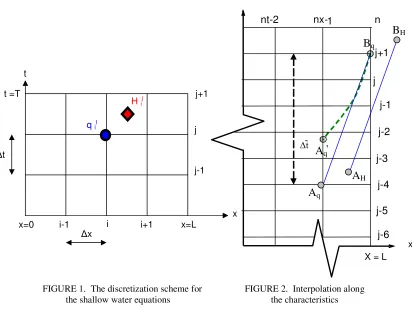
are values located at interior points as described below.FIGURE 1. The discretization scheme for the shallow water equations
FIGURE 2. Interpolation along the characteristics
Figure 1 shows the relative locations of the variables q and H in the space and time staggered mesh. Figure 2 shows the locations Bq of qj+1nx which is available from the time stepping calculations and the location BH of Hj+1nx which is unknown and so must be obtained by interpolation back along the characteristic path BA. That is, path BqAq is used to find
q
~
and path BHAH is used to find H~ using MOC.The standard (MOC) will determine
q
~
at location Aq andH
~
at location AH at x=(nx−1)∆xand time t CFL j tnx∆ =
∆~ (1/ ) earlier than at Bq and BH respectively, where(CFL)nxj =(c+u)nxj (∆t/∆x). That is, the characteristic path is assumed to be straight. The (MMOC), however, traces the paths to A'q and A'H by tracking the characteristic through a series of small intervals tk t
~
∆ <
∆ , see Figure 3. The CFL is re-estimated at each interval by interpolation of u and H from neighbouring cells. In this way, the path is curved and more accurate values of q~ and H~ are found. In relatively deep water for which
x t x j-1 j j+1 x=L
x=0 i-1 i i+1
t =T t
q ij
H ij
x = L
x 1
+ j nx
H
j+1
j
j-1 nx nx-1
k2
k1
kp
j-3
k3
j-2
variations in H are small then MOC provides good results with insignificant reflections. However, when H varies from perhaps 0.01 m. (almost dry bed) to 2.0 m. or more during the simulation of a flash flood in a "dry" river bed then the characteristic path is locally curved due to the effect of the nonlinearity. In this situation MOC gives poor results. By taking a set of suitably small intervals ∆tk the MMOC can reduce reflections to a satisfactory level even when sharp changes in flow conditions approach the boundary.
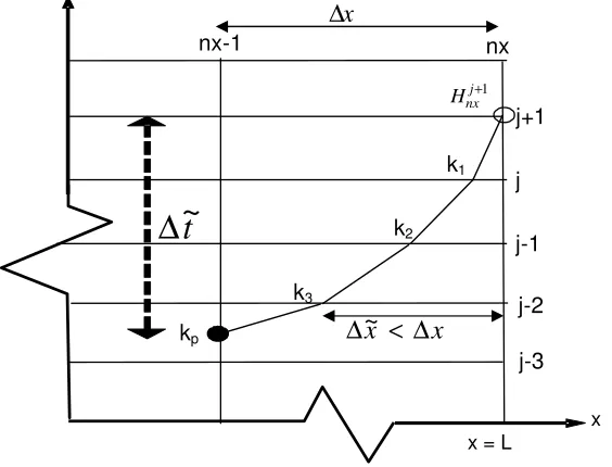
3.3 –Theory and Governing Equations of the Modified Method of Characteristics (MMOC)
[image:4.612.161.443.343.558.2]The main idea behind the algorithm of (MMOC) is to calculate the time interval ∆t~accurately using the geometry illustrated at Figure 3. Updated calculations of both the water depth and discharge are used to evaluate the celerity of the wave, c and the water velocity, u and hence CFL at each partial step k1, k2, k3 etc. The last available computed value of H is at node (nx, j) while it required to evaluate the downstream boundary value of H at node (nx, j+1) as indicated by the diamond. From equation 3.5 it can be seen that values of q~ and H~ are needed at a time∆~t earlier. Therefore, the main aim is to track the path of the characteristic back in time and space by locating all the points (k) until we locate the last point (kp) as shown in Figure 3. The necessary checks are carried out at each time step to ensure that∆~x < ∆x. If ∆x~ ≥ ∆x then the trajectory has intersected the vertical line one space step back, i.e. at nx-1. At this stage a direct interpolation between q(nx-1,j-2) and q(nx-1,j-3) is used to evaluate the discharge
q
~
at point (kp). A similar interpolation can be used to findH~ . Then the value of H(nx,j+1) can be found by propagating along the forward characteristic starting at H~ using equation 3.4 step by step from kp,..,k3, k2, k1 as indicated in equation 3.6:FIGURE 3. Interpolation along the characteristics using the (MMOC)
[
2]
11
) (
1
−
−
∂ ∂ + +
∆ − − +
= k k
k
x z gH H
q q k q u c H
H
(3.6)
Where ∆q= qk −qk−1 also along the characteristic path.
This equation is implemented at each time step to evaluate the value of H at the advanced time beginning from point (kp) and ends by providing the required value of the water depth at node (nx,j+1),
1 + j nx
H . The main advantages of MMOC are:
x
x
<
∆
∆
~
t
~
∆
x
1- The appropriate allocation of the starting point (kp) using a simple interpolation at each time step backward in time and space
2- It follows the correct path of the characteristic, i.e., at all the points (k), the wave celerity and the water velocity are updated to evaluate the correct value of CFL. As a result of this, the MMOC approaches the correct path of the characteristic in its curved shape much better than the common MOC.
As expected the efficiency of the MMOC increase as the nonlinearity of the shallow water equation increases. In other words, as the ratio of the peak flood event to the initial water depth increases as discussed later in the simulation cases.
4- Model verifications
4.1 Introduction
Developing a complete test to check and validate an exact solution for the nonlinear Shallow Water Equations (SWE) is not possible. It is possible however to develop simple tests to compare the model results with analytical solutions of certain idealised cases. Several tests have been carried out to verify the model from uniform steady flow to non-uniform unsteady flow, we will mention here just the two most important tests.
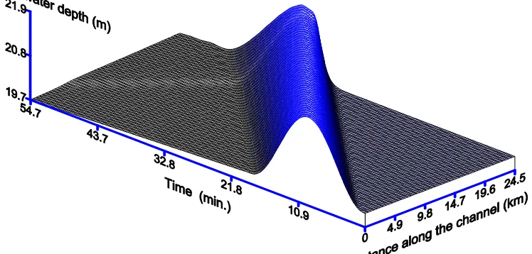
4.2 Validation test 1 – non-uniform unsteady flow
[image:5.612.125.495.390.575.2]The main objectives of this test are to ensure that the value of both the discharge (q) and the water depth (H) entering at the upstream boundary propagate downstream without any change and the relationship between q and H follows the analytical solution of the shallow water wave. The results of the model are a driving upstream boundary hydrograph of peak discharge q = 28.24 m3/s/m. The calculated upstream boundary hydrograph has a peak value, H max = 21.96 m. while the wave speed is 14.74 m/s.
FIGURE 4. Water depth (H) within the domain
4.3 Validation test 2 - Unsteady flow within a sloping channel and rough bed
The objective of this test is simply to look for the whole channel as a control volume to ensure that there are no significant losses or accumulation in volume within the simulated domain. The results of this test are not compared with the analytical solution only, but are compared with other model results as well. If we consider the initial water depth is Hi and at the end of the simulation is Hf, while the driving discharge upstream is qu and downstream is qd. So, we can say the total net volume entering the channel is ∆V1=
∫
qu dt−∫
qd dt, while the total volume change in the channel is∫
∫
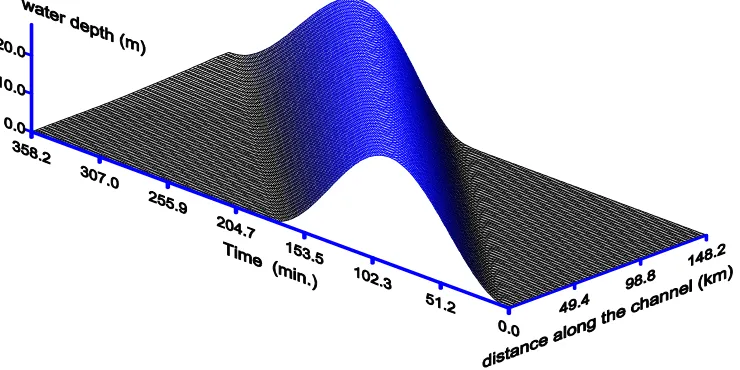
− =∆V2 Hf dx Hidx. For equilibrium, we should have ∆V1=∆V2. The model was applied for non-uniform unsteady flow conditions within a sloping channel and a rough bed. The initial water depth was chosen H initial = 20.0 m. The result of the flood wave propagation within the domain is presented at Figure 5. From the simulation of this event it was found that:
95 . 5284
1= − =
∆V
∫
qd dt∫
qu dt m3/m. and ∆V2=∫
Hidx−∫
Hf dx=5330.36m3/m. So, 41. 45 1 2−∆ ≅
[image:6.612.128.502.278.457.2]∆V V m3 ≈ 0.86 ٪ which is acceptable and it is very small error compared to several previously developed models such as Abiola (1988) which overestimated by 28 %.
Figure 5. Water depth (H) within the domain
5 - Test cases
5.1 - Introduction
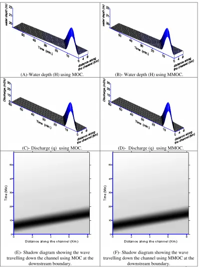
Two cases will demonstrate the benefits of the (MMOC) over (MOC). As the advantages arise when the peak flood height (HP) is large compared with the initial water depth (H0), the cases will be characterized by the ratio (R= HP/ H0). The first case has R = 0.1 when we expect the (MOC) and (MMOC) to perform equally well and the second case has R = 22.2 which will demonstrate the improvements from uses (MMOC).
5.2 - Case 1:
(A)-Water depth (H) using MOC. (B)- Water depth (H) using MMOC.
(C)- Discharge (q) using MOC. (D)- Discharge (q) using MMOC.
(E)- Shadow diagram showing the wave travelling down the channel using MOC at the
downstream boundary.
(F)- Shadow diagram showing the wave travelling down the channel using MMOC at the
[image:7.612.110.509.63.600.2]downstream boundary.
Figure 6. Water depth within the domain (m.) and discharge per unit width within the domain (m2/s.)
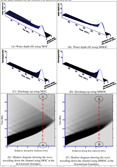
5.3 - Case 2:
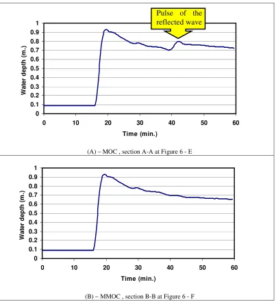
considerable reflected wave. While on the other hand, it is clear from Figure 7- B, D and F that the wave ‘sees’ the downstream boundary as being transparent. Figure 8 illustrates the water depth downstream for both MOC and MMOC at distance equal to 3.3 Km from the upstream boundary and it is found that at time 43 min the amplitude of the reflected wave is about 10 cm which is about 14.3 % from the water depth at this location, or about 87 % of the approaching wave, when the downstream values are interpolated using (MOC) as shown in section (A-A), while there is no discernable reflection at the same location for the (MMOC) as shown in section (B-B).
(A)-Water depth (H) using MOC. (B)- Water depth (H) using MMOC.
(C)- Discharge (q) using MOC. (D)- Discharge (q) using MMOC.
(E)- Shadow diagram showing the wave travelling down the channel using MOC at the
downstream boundary.
(F)- Shadow diagram showing the wave travelling down the channel using MMOC at the
[image:8.612.108.504.142.709.2]downstream boundary.
Figure 7. Water depth within the domain (m.) and discharge per unit width within the domain (m2/s.)
A
B
0 0.1 0.2 0.3 0.4 0.5 0.6 0.7 0.8 0.9 1
0 10 20 30 40 50 60
Time (min.)
W
a
te
r
d
e
p
th
(
m
.)
(A) – MOC , section A-A at Figure 6 - E
0 0.1 0.2 0.3 0.4 0.5 0.6 0.7 0.8 0.9 1
0 10 20 30 40 50 60
Time (min.)
W
a
te
r
d
e
p
th
(
m
.)
[image:9.612.106.509.75.517.2](B) – MMOC , section B-B at Figure 6 - F
Figure 8. water depth at 2.65 Km from the upstream boundary for both MOC and MMOC
6 - SUMMARY AND CONCLUSION:
A simple shallow water equation solver is presented, that is able to simulate sharply rising flood events producing stable, mass conserving solutions. The usual problem with limited domain models produces reflections from the downstream boundary which should be completely transparent. Interpolation of boundary values using (MOC) is often used. However, as commonly implemented, significant reflection occurs when large amplitude flood waves arrive at the boundary.
The paper presents a modified method of characteristics which tracks the characteristic path carefully by means of a series of small increments to locate the correct values in the domain for interpolation to the boundary. Results demonstrate that this relatively simple enhancement to a well known method produces very good results with undetectable reflections for cases of large flood waves
REFERENCES ABBOTT, M.B. 1977.
An Introduction to the Method of Characteristics, Thames and Hudson, London UK. ABIOLA, A.A. AND NIKALOAOS, D.K. 1988.
Model for Flood Propagation on Initially Dry Land, ASCE Journal of Hydraulic Engineering, vol. 114, No. 7
COURANT, R., FREDRICHES, K.O., LEWY H. 1928.
Uber die partiellen Differenzengleichungen der mathematischen Physik, Math. Ann., Vol.100,32-74 (in german)
DELIS, A.I., SKEELS, C.P. AND RYRIE, S.C. 2000.
Evaluation of some approximate Riemann solvers for transient open channel flows, Journal of Hydraulic Research, vol. 38, No 3, 217–231.
ERDURAN, K.S., KUTIJ, A. V. AND HEWETT, C.J.M. 2002
Performance of Finite volume solutions to the shallow water equations with shock capturing schemes. International Journal for Numerical Methods in Fluids, Vol. 40, 1237–1273.
FALCONER, R.A. AND LIU, S.Q. 1988.
Modeling Solute Transport Using QUICK Scheme, ASCE J. of Environmental Engineering, vol. 114, 3-20. FLETCHER, C.J. 1991A.
Computational Techniques for Fluid Dynamics 1: Fundamental and General Techniques,
Springer-Verlang.
FLETCHER, C.J. 1991B.
Computational Techniques for Fluid Dynamics 2: specific Techniques for Different Flow Categories, Springer-Verlang.
FRENCH, R.H. 1986.
Open Channel Hydraulics, McGraw Hill. GLAISTER, P. 1988.
Approximate Riemann solutions of the shallow water equations. Journal of Hydraulic Research,vol. 26, 3, 293 –306.
GOUTAL, N. AND MAUREL, F. A. 2002
Finite volume solver for 1D shallow water equations applied to an actual river. International Journal for Numerical Methods in Fluids, vol. 38, 1–19.
LEONARD, B.P. 1983.
Third-Order Upwinding as a Rational Basis for Computational Fluid Dynamics; Computational Techniques & Applications, CTAC-83, Edited by Noye, J. And Fletcher, C., Elsevier.
SANDERS, B. AND KATOPODES, N. 2000.
Adjoint Sensitivity Analysis for Shallow Water Wave Control, J. of Engineering Mechanicsvol. 126 (9), 909–919
CHANG, F.F.M., AND RICHARDS, D. L. 1971.
Deposition of Sediment in Transient Flow, J. Hydr. Dev., ASCE, 97 (HY6),837-849
VARDY, A. E. 1977.
On the Use of The Method of Characteristics for the Solution of Unsteady Flows in Networks, Proc., 2nd Int. Conf on Pressure Surge, British Hydromech. Res. Assoc., Fluid Engineering, Cranfield, England, (H2),15-30
WYLIE, E. B. 1980.
Inaccuracies in the Characteristics Method, Proc., 28th, Annual Hydraulic. Spec. Conf., ASCE, Chicago, III.,
165-176
GOLDBERG, D. E. AND WYLIE, E. B. 1983.