Boundary Superstring Field Theory Annulus Partition Function in the Presence of Tachyons

      

City, University of London Institutional Repository

Citation

:

Arutyunov, G., Pankiewicz, A. & Stefanski, B. (2001). Boundary Superstring Field Theory Annulus Partition Function in the Presence of Tachyons. Journal of High Energy Physics, 2001(JHEP06), 049. doi: 10.1088/1126-6708/2001/06/049

This is the accepted version of the paper.

This version of the publication may differ from the final published

version.

Permanent repository link:

http://openaccess.city.ac.uk/12560/

Link to published version

:

http://dx.doi.org/10.1088/1126-6708/2001/06/049

Copyright and reuse:

City Research Online aims to make research

outputs of City, University of London available to a wider audience.

Copyright and Moral Rights remain with the author(s) and/or copyright

holders. URLs from City Research Online may be freely distributed and

linked to.

City Research Online: http://openaccess.city.ac.uk/ [email protected]

arXiv:hep-th/0105238v2 28 May 2001

hep-th/0105238 AEI-2001-054

Boundary Superstring Field Theory Annulus

Partition Function in the Presence of Tachyons

G. Arutyunov

∗ †

, A. Pankiewicz

‡

, B. Stefa´

nski, jr.

§

Max-Planck-Institut f¨ur Gravitationsphysik, Albert-Einstein Institut Am M¨uhlenberg 1, D-14476 Golm, Germany

May 2001

Abstract

We compute the Boundary Superstring Field Theory partition function on the annulus in the presence of independent linear tachyon profiles on the two boundaries. The R-R sector is found to contribute non-trivially to the derivative terms of the space-time effective action. In the process we construct a boundary state description of D-branes in the presence of a linear tachyon. We quantize the open string in a tachyonic background and address the question of open/closed string duality.

∗_{E-mail address: [email protected]}

†_{On leave of absence from Steklov Mathematical Institute, Gubkin str.8, 117966, Moscow, Russia} ‡_{E-mail address: [email protected]}

1

Introduction

In the last few years significant progress has been made in understanding the open string tachyon dynamics. It has become clear that open string tachyon condensation describes the decay of un-stable D-branes into un-stable ones or into the closed string vacuum. Initially the discussion was based on the first quantized string theory [1, 2, 3]. Subsequently tachyon condensation has been investigated with a remarkable degree of accuracy in Cubic Open String Field Theory [4] by using the level truncation approximation [5]. From the world-sheet point of view the tachyon conden-sation process is then viewed as the RG flow relating conformal field theories with Neumann and Dirichlet boundary conditions [6, 7]. More recently it has been argued [8, 9, 10, 11, 12, 13, 14] that the Boundary String Field Theory (BSFT) [15, 16] also provides a suitable description of the tachyon condensation. In particular the exact tree level tachyon potential, the ratios of the brane tensions [8, 9] as well as the low-energy effective action for massless fluctuations around a tachyonic soliton [17] are obtained quite naturally in this setting.

A basic object of the BSFT is an effective space-time action Seff considered as a functional

of the open string background fields. In the supersymmetric case, with which we will be mainly concerned here, the BSFT action is known [11, 18, 19, 20] to coincide with the partition function Z of the open string boundary sigma model [21]. In the sigma model approach the Weyl and diffeomorphism invariant string action on a world-sheet Σ with boundaries is modified by includ-ing boundary perturbations which correspond to turninclud-ing on space-time background fields. For example one may turn on a background gauge fieldAµ by including a boundary perturbation1

Sgauge=−i

Z

∂Σds Aµ(X)

∂ ∂sX

µ_{, (1.1)}

This perturbation is marginal as it preserves both Weyl and diffeomorphism invariance. In the study of the open superstring background tachyon one includes a boundary perturbation

Stachyon=

1 2 Z

∂Σds T

2_{(X), (1.2)}

where T(X) is a tachyon profile. A particularly simple case is the linear profile T(X) = uµXµ,

for some non-negative constantsuµand dsis the diffeomorphism invariant length element on the

boundary∂Σ of the world-sheet. In this case the boundary sigma model is exactly solvable. The higher open string background fields can also be incorporated in this approach [22] though the corresponding action defines a non-renormalizable theory.

One important part of the investigation of the supersymmetric boundary sigma model is a study of contributions of higher genus Riemann surfaces toZ. This should give new insight into the effective action Seff, provided that the correspondence Seff = Z holds for higher Riemann

1

surfaces as well. In this paper we consider the case of the annulus, a subject already being under discussion in the current literature [23]-[27].

In general one defines (as in the case of Polyakov’s string [28]) the path integral to include an integration over world-sheet metrics, modulo the symmetries of the theory. In particular the sigma model action is still invariant with respect to a subgroup of the diffeomorphism group compatible with the boundary conditions. The boundary action (1.2) is not Weyl-invariant, while the bulk action is. This too should be accounted for in a path integral formulation. Since such a path integral formalism, properly accounting for the remaining gauge symmetry, is not presently available, the first problem to study is to consider some fixed metric gαβ on the annulus and to

compute Z[gαβ], the path integral over the Xµ’s.

In this paper we consider the simplest case of the flat metric on the annulus for which the bosonic part of the action is (we setα′ _{= 2)}

S = 1

8π Z 1

a

Z 2π

0 rdrdφ

1

r2(∂φX(r, φ)) 2

+ (∂rX(r, φ))2

+ 1 8πuµuν

Z 2π

0 dφX

µ_Xν_{(1, φ) +} 1

8πavµvν Z 2π

0 dφX

µ_Xν_{(a, φ), (1.3)}

whereu , v are tachyons on ther = 1 and r=a≤1 boundaries of the annulus, respectively; the presence of a in the last term of the action is due to the diffeomorphism invariant measure ds. A more detailed discussion of the action involving fermions will be given in Section 2.

The computation of the annulus partition function can be done in several ways and below we briefly summarise those used in this paper. Perhaps the most direct approach is via the Green’s function method, discussed in Section 3. The classical field configurations minimizing the bosonic action (1.3) are subjected to the following boundary conditions2

∂rXµ(1, φ) +uµuνXν(1, φ) = 0, −∂rXµ(a, φ) +vµvνXν(a, φ) = 0 (1.4)

and computing the path integral by the Green’s function approach one may conveniently choose the Green’s functions to obey the same type of boundary conditions. The two limiting cases u= 0,∞ correspond to Neumann and Dirichlet boundary conditions, respectively.

In Section 3 we derive the boundary conditions for fermions, taking into account the differ-ent spin structures on the annulus. In particular we show that the choice of spin structure is equivalent to identifying the boundary fermion, treated as a Lagrangian multiplier, in terms of the bulk fermions. In Section 3 we construct the Green’s functions both in the NS-NS and R-R sectors for different spin structures and use them to derive the corresponding contributions to the partition function.3

2

Our boundary conditions differ from the ones used in [23, 25, 27]. They do agree with [24] and [26] who also use the diffeomorphism invariant measure.

3

In Section 4 we discuss another way to compute the partition function. We map the annulus to the cylinder via

τc = lnr , σc =φ , (1.5)

and construct boundary states [29, 30]_|B, u_i,_hB, v_|corresponding to the absorption and emission of closed strings from the D-branes with background tachyons turned on.4 _{Specialising to a}

tachyon profile withuµandvµin the same direction (sayµ= 9) the bosonic part of the boundary

states (in that direction) satisfy

∂τcX9(1, σc) +u2X9(1, σc)

|B, u,0i= 0, hB, v,−l|−∂τcX9(l, σc) +av2X9(l, σc)

= 0,

(1.6) with l=−lna. The partition function on the cylinder is

Zcylinder(u, v) =

Z ∞

0 dlhB, v|e

−lHc

|B, ui, (1.7)

where Hc is the (conformal) closed string Hamiltonian. In this formalism the disc partition

function is

Zdisc(u) =hvacuum|B, ui, (1.8)

which can be shown to coincide with the one computed in [8, 9, 11, 15]. The boundary state approach emphasizes the conformal nature of the bulk theory - in the bulk the usual Virasoro generators Ln,L˜n are well defined and satisfy the standard algebra. For a conformal boundary

perturbation the boundary states satisfy [32]

(Ln−L˜−n)|Bi= 0, (1.9)

indicating that Weyl invariance is not broken on the boundary. The|B, uisatisfy no such simple relation.

The construction of the boundary states involves finding suitably normalized coherent states which satisfy (1.6) and fermionic boundary conditions in the NS-NS and R-R sectors. These states have to be invariant under the closed string GSO projection. Due to the presence of fermionic zero-modes this places a restriction on the allowed boundary states in the R-R sector [3]. In particular it is well known that with no background tachyon the Dp-brane R-R boundary state is GSO invariant for p even/odd in Type II A/B, respectively. So for example there is no GSO invariant R-R boundary state corresponding to the non-BPS D9-brane of Type IIA. We show that in the presence of a non-zero background tachyon in one direction (say u9 _{6= 0) a GSO}

invariant non-BPS D9-brane R-R boundary state does exist. The normalization of this state depends linearly onu9 _{and so becomes zero in the non-BPS D9-brane limit. In the limitu}9 _{→ ∞}

it reduces to the boundary state of the BPS D8-brane.

4

Finally, we change coordinates on the annulus again, taking the world-sheet time to be peri-odic

σo =−τc

π

l , τo =σc π

l , (1.10)

and compute the functional integral on the annulus as an open string partition function. In this case the boundary conditions are

∂σoX9(τo,0)−

u2_l

π X

9_(τ

o,0) = 0, ∂σoX9(τo, π) +

av2_l

π X

9_(τ

o, π) = 0. (1.11)

In the first part of Section 5 the open string on a strip with boundary conditions relevant to tachyonic perturbations is analysed. The system is canonically quantised and found to have a countably infinite spectrum. Our partition function is found to factorise on closed string poles (with residues depending on the tachyons) giving it the interpretation of a transition amplitude for a closed string propagating between two non-BPS D9-branes in the presence of background tachyons. We compute a renormalised, tachyon dependent normal-ordering constant of the open string Hamiltonian which we expect to be compatible with the open/closed string duality. The path integral on the annulus is then computed as an open string partition function with boundary conditions (1.11) in the second part of the section. Some details about Green’s functions and the derivation of the partition function are relegated to the Appendix.

To summarise, we compute the superstring partition function on the annulus in the presence of background open string tachyonic fields and show in particular that the R-R sector contributes non-trivially. In the process we construct boundary states in the presence of linear tachyons; as a corrolary we compute the WZ couplings of non-BPS D-branes. Furthermore we discuss the quantisation of an open string in the presence of a background tachyon, comment on the fate of the open string GSO projection and open/closed string duality.

2

The superstring action in a tachyon and gauge field

background

The world sheet action for the superstring in the background of a tachyon and abelian gauge field is

S =Sbulk+Sbndy, (2.1)

with the standard NSR action in the bulk (we set α′ _{= 2)}

Sbulk =

1 4π

Z

Σ d 2_z

∂zXµ∂z¯Xµ+ψµ∂z¯ψµ+ ˜ψµ∂zψ˜µ

, (2.2)

and the boundary action in superspace [11], [14]

Sbndy=−

1 2π

Z

∂ΣdsdΘ

ΓDΓ +T(X)Γ + i

2Aµ(X)DX

The boundary superspace coordinates are (s,Θ), where Θ is the boundary Grassmann coordinate and s =rφ, φ being the angular coordinate on the boundary. Here X = X+ Θθ, where θ is a boundary fermion, whose precise relation to the bulk fermionsψ and ˜ψ will be determined below and D=∂Θ+ Θ∂s. Γ =ρ+ ΘK is an auxiliary boundary superfield [2, 6].

The world-sheet Σ is the annulus with inner radius a < 1 and outer radius equal to one. In this case there is generically an independent set of background and auxiliary fields on each component of the boundary, though to avoid cluttering of notation this is not explicitly indicated in the above. Performing the integral over Θ and integrating out the auxiliary fieldK one obtains

Sbndy =−

1 2π

Z

∂Σds

˙

ρρ+∂µT(X)θµρ−

1 4T(X)

2₊ i

2Aµ(X) ˙X

µ₊ i

4Fµν(X)θ

µ_θν_{, (2.4)}

where ˙ρ=∂sρetc. The world-sheet theory is exactly solvable in the presence of a linear tachyon

profile and a constant abelian field strength

T(X) =uµXµ, Aµ(X) =−

1 2FµνX

ν_{. (2.5)}

In this case the boundary action is

Sbndy =

1 8π

Z

∂Σds(uµνX

µ_Xν_+iF

µν∂sXµXν −iFµνθµθν −4∂sρρ−4uµθµρ), (2.6)

where we defined uµν ≡uµuν.

The relationship between the boundary and bulk fermions can be determined as follows. On-shell the variation of the fermionic bulk term reduces to the boundary contribution

δSbulk =−

i 4π

Z

dsψµ(s)δψµ(s) + ˜ψµ(s)δψ˜µ(s)

, (2.7)

where we took into account the transformation of the bulk fermions from z = reiφ _{to s = rφ}

variables. As above we introduce the boundary action with the boundary fermion θ, which is a new field and relate it to the bulk fermions by treating it as the Lagrange multiplier in the following modified boundary action

S′

bndy=Sbndy−

i 8π

Z

∂Σds θ

µ_(ψ

µ−iηψ˜µ), (2.8)

with η = _±1. As we will see in a moment this (and a similar choice ˜η = _±1 on the other component of the boundary) corresponds to the spin structure, since it leads to different ways of identifying the boundary fermion in terms of the bulk fermions.5 _{Introducing ψ}

±=ψ±iηψ˜the

variation coming from the fermionic parts of the action now reads (on the r= 1 boundary)

δS =₋ i 8π

Z

dφhψ−δψ++ (ψ++θ)δψ−−ψ−δθ

i

+δSbndy. (2.9)

5

We define the boundary conditions for fermions by requiring the variation of the total action to vanish on-shell. Since δψ− and δθ are independent variables on the boundary the vanishing of

the coefficient of δψ− yields

−θ =ψ+ =ψ +iηψ,˜ (2.10)

i.e. it now relates the bulk and boundary fermions. This relation implies δψ+ = −δθ and the

remaining part of δS gives the boundary conditions for θ (cf. Section 3).

The choice of boundary fermion ₋θ = ψ +iηψ˜ in terms of bulk fermions is precisely the choice of spin structure. Since we have two boundaries for the annulus we have in sum four different possibilities to identify the boundary fermions with the bulk fermions (cf. [30]). These cases should be combined with the conditions for bulk fermions to be antiperiodic or periodic around the circle, so together we would get eight different sectors. However, as we will show in Section 3, there are only four different sectors since the spin structure enters in the final answers only through the combination ηη˜.

3

The annulus partition function via Green’s functions

In this section we determine the complete partition function in the closed channel by the method of Green’s functions [33]. For the sake of clarity we will analyse the different sectors separately and summarise the results here. The computational details are presented in the Appendix.

3.1

The bosonic sector

Besides the Laplace equation in the bulk theXµ_{’s satisfy}6

(z∂z+ ¯z∂z¯)Xµ+uµνXν +Fµν(z∂z−z∂¯ z¯)Xν = 0, |z|= 1,

−(z∂z + ¯z∂¯z)Xµ+avµνXν +Lµν(z∂z−z∂¯ z¯)Xν = 0, |z|=a , (3.1)

where z = reiφ_{, L}

µν and vµν = vµvν are respectively the gauge field and tachyon on the r = a

boundary. The Green’s function corresponding to these boundary conditions is

G(z, w) = ₋ln_|z₋w_|2+A₋ 1

2Culn|z|

2_ln

|w_|2+Cln_|z_|2+CT ln_|w_|2

+ X

k>0

(αkzk+α−kz−k+ ˜αkz¯k+ ˜α−kz¯−k), (3.2)

where

A = 2(1₋avlna)(u+av₋auvlna)−1, (3.3)

C = av(u+av₋auvlna)−1. (3.4)

6

The normal and tangential derivatives are∂r= |1z|(z∂z+ ¯z∂z¯), ∂s=

i

The explicit expressions for the oscillators are given in the Appendix . G(z, w) satisfiesGµν(z, w) =

Gνµ(w, z) and is in fact the propagatorhXµ(z)Xν(w)i.

One finds the bosonic contribution to the partition function (up to normalization) by differ-entiating the boundary action (2.6) with respect to the world-sheet couplings [15] and using this Green’s function (for more details see the Appendix). The resulting expression is

Zbos(a) = det(u+av−auvlna)−1/2

∞

Y

k=1

det(1 +u/k+F)−1det(1 +av/k+L)−1

× det1−a2kSk(u, F)Sk(av, L)

−1

, (3.5)

where

Sk(u, F) =

k₋u₋kF

k+u+kF . (3.6)

This result is purely formal and has to be regularized. The infinite product above diverges and is treated in Section 4.2 (cf. equations (4.30) and (4.31) below). As in the disc case the bosonic and fermionic divergences combine to produce a finite result [11, 12, 14]. Furthermore the matrix (u+av−auvlna) has rank one or two depending on whether the tachyons uµ, vµ are switched

on in one or more directions.7 _{The determinant above should be understood as a product of}

the determinant of the maximal rank sub-matrix and the regularised volume of the remaining space-time directions.

In principle there may also be an overall dependence on the modulus a in the partition function that could not be fixed by the previous considerations. By looking at the change of the action under variations of the modulus [33] one can also derive an equation for∂alnZ. It turns

out that this equation is consistent with the above expression (3.5) for the partition function,

i.e.no extra dependence on aappears (for details see the Appendix). Note also that in the limit a→0 one recovers the (bosonic) partition function on the disc (setting L= 0) [15].

The partition function obtained above agrees with the one computed in section 4 using the boundary state formalism. When comparing the two results one should note that the correct integration measure on the annulus is da_a2.

3.2

The NS-NS sector

In the NS-NS sector neither ρ nor θ have zero-modes and the auxiliary boundary fermion ρ can be integrated out. The fermionic part of the boundary action becomes

S′F_bndy = 1 8π

Z

∂Σ

uµνθµ∂s−1θν −iFµνθµθν −iθµ(ψµ−iηψ˜µ)

, (3.7)

7

and the fermionic boundary conditions following from the (on-shell) vanishing of the total vari-ation of Sbulk +Sbndy′ (cf. the discussion in Section 2) are

δµν+iuµν∂s−1+Fµν

ψν = iηδµν −iuµν∂s−1−Fµν

˜

ψν, r= 1,

δµν −iavµν∂s−1−Lµν

ψν = iη˜δµν +iavµν∂s−1+Lµν

˜

ψν, r =a . (3.8)

Introducing the four kinds of Green’s functions on the boundaries

G++(z, w) ≡ hψ(z)ψ(w)i=−i

√

zw z₋w +

∞

X

r=1/2

(ψr(w)zr+ψ−r(w)z−r),

G−−(¯z,w¯) ≡ hψ˜(¯z) ˜ψ( ¯w)i=−i √

¯ zw¯ ¯

z₋w¯ +

∞

X

r=1/2

( ˜ψr( ¯w)¯zr+ ˜ψ−r( ¯w)z−r),

G+−(z,w¯) ≡ hψ(z) ˜ψ( ¯w)i= ∞

X

r=1/2

(ar( ¯w)zr+a−r( ¯w)z−r),

G−+(¯z, w) ≡ hψ˜(¯z)ψ(w)i=

∞

X

r=1/2

(br(w)¯zr+b−r(w)¯z−r), (3.9)

the boundary conditions on the Green’s functions can be written as

(1 +F)z∂z +u)G+±+iη((1−F)¯z∂¯z+u)G−± = 0, |z|= 1,

(₋(1₋L)z∂z+av)G+±+iη˜(−(1 +L)¯z∂z¯+av)G−± = 0, |z|=a. (3.10)

The boundary fermion at r = 1 is related to the bulk fermions by θ = ₋(ψ +iηψ˜) (cf. equa-tion (2.10)) and therefore the propagator is

hθθi=G++−G−−+iη(G+−+G−+). (3.11)

On the boundaryr =a the second boundary fermion ˜θ is ˜

θ =₋(ψ+iη˜ψ˜) (3.12)

and consequently has propagator

hθ˜θ˜_i=G++−G−−+iη˜(G+−+G−+). (3.13)

A straightforward, though tedious calculation determines the oscillators of the Green’s functions (whose explicit expressions are again collected in the Appendix) and, using the expressions for the boundary fermion propagators, one finds that the resulting contribution to the partition function from the NS-NS sector spin structures is formally

ZNS-NS(a, ηη˜) =

∞

Y

r=1/2

det(1+u/r+F)det(1+av/r+L)det1₋ηηa˜ 2rSr(u, F)Sr(av, L)

Due to the closed string GSO projection the contributions from different spin structures (ηη˜=

±1) should be added with the opposite sign. This removes the closed string tachyon (cf. Sec-tion 4).

3.3

The R-R sector

The R-R sector is more subtle, due to the appearance of theρ andθ modes. Since the zero-mode drops out of the kinetic term of the auxiliary boundary fermion ρ one cannot integrate out ρ completely as in the NS-NS sector. Instead we will integrate out the non-zero modes and treat the zero-modes separately. Then the boundary condition on the non-zero modes of ψ, ˜ψ are exactly as in (3.8). The Green’s functions now read

G++(z, w) ≡ hψ(z)ψ(w)i

= ₋i 1

z₋w(wΘ(|z| − |w|) +zΘ(|w| − |z|)) +

∞

X

r=1

(ψr(w)zr+ψ−r(w)z−r),

G−−(¯z,w¯) ≡ hψ˜(¯z) ˜ψ( ¯w)i

= −i 1 ¯

z−w¯( ¯wΘ(|z| − |w|) + ¯zΘ(|w| − |z|)) +

∞

X

r=1

( ˜ψr( ¯w)¯zr+ ˜ψ−r( ¯w)z−r),

G+−(z,w¯) ≡ hψ(z) ˜ψ( ¯w)i= ∞

X

r=1

(ar( ¯w)zr+a−r( ¯w)z−r),

G−+(¯z, w) ≡ hψ˜(¯z)ψ(w)i=

∞

X

r=1

(br(w)¯zr+b−r(w)¯z−r), (3.15)

where Θ(|z| − |w|) is the step function. A completely analogous calculation to the one for the NS-NS sector shows that the contribution of the R-R non-zero modes to the partition function is

ZR-R(a, ηη˜) =

∞

Y

r=1

det(1 +u/r+F)det(1 +av/r+L)det1−ηηa˜ 2rSr(u, F)Sr(av, L)

. (3.16)

For the zero-modes the kinetic terms of the auxiliary boundary fermionsρ, ˜ρare absent and the relevant part of the boundary action reads8

S_bndy(0) =₋ 1 8π

Z

∂Σds(4uµθ

µ

0ρ0+iFµνθ0µθ0ν). (3.17)

Integrating out ρ0 and ˜ρ0 we have

Z_R-R(0) =

uµθ0µexp(

i 4Fρλθ

ρ

0θ0λ)

r=1

avµθ˜µ0 exp(

i 4Lρλθ˜

ρ

0θ˜0λ)

r=a

. (3.18)

8

Translating this into Hilbert space language, we see that the zero-mode part of the partition function in the R-R sector is given by the amplitude of the “in-states” at r = a and the “out-states” atr= 1. The explicit expression for the in- and out-states will be derived in the following. The zero-modes of the bulk fermions satisfy

{ψ₀µ, ψ₀ν_}=δµν =_{ψ˜₀µ,ψ˜ν_0}, _{ψ₀µ,ψ˜ν_0}= 0. (3.19)

The action ofψ₀µ and ˜ψ₀µ on the R-R vacuum (in a non-chiral basis)

|A,B˜_{i ≡} lim

z,¯z→0S

A_{(z) ˜S}B_(¯z)

|0_i, A, B = 1, . . . ,32 (3.20)

can be realized as9

ψµ0|A,B˜i =

1

√

2(Γ

µ₎A

C(1)BD|C,D˜i,

˜

ψµ0|A,B˜i =

1

√

2(Γ11)

A

C(Γµ)BD|C,D˜i. (3.21)

The vacuum ‘in-state’ is defined by the free boundary condition

(ψµ0 −iη˜ψ˜0µ)| −η˜i= 0. (3.22)

Explicitly it is

| −η˜i=MAB(˜η)|A,B˜i, M

(˜η)

AB =

" CΓ11

1 +iη˜Γ11

1 +iη˜ #

AB

, (3.23)

where C is the charge conjugation matrix. Similarly, the vacuum “out-state” is

hη_|=_hA,B˜_|NAB(η), _NAB(η) =₋ "

CΓ11

1₋iηΓ11

1 +iη #

AB

, (3.24)

and satisfies

hη_|(ψ0µ+iηψ˜0µ) = 0. (3.25)

We have

hη_{| −}η˜_i=₋32δη,−η˜, (3.26)

so that, as usual, only one of the two spin structure contributions of the R-R sector is non-zero. Since the boundary fermions anti-commute the expansion of the exponentials will in general terminate at fourth order in the gauge field strengths and we have

Z_R-R(0) =auµvνhθ0µ|θ˜0νi −

1

16auµvνFρλLστhθ

µ

0θ

ρ

0θ0λ|θ˜0νθ˜0σθ˜0τi+· · · (3.27) 9

Since ˜θµ₀ and θµ₀ act as creation and annihilation operators on the in and out vacua respectively, only terms with the same number of θ0µ and ˜θ0µ give a non-zero contribution. We explicitly

compute this in two particular cases. First consider turning on tachyons u , v in directions transversal to a gauge field L=F. In this case the zero-modes contribute as

Z_R-R(0) _∼auµvµdet(1 +F). (3.28)

Next consider againL=F restricted to, say, four directionsµ= 1,2,3,4 with the tachyons non-zero in the same directions. As long as the tachyons u, v are general we may in fact rotateF to bring it to a block-diagonal form consisting of two antisymmetric 2_×2 matrices with independent entries f1, f2. After some algebra the result becomes

Z_R-R(0) _∼auivi+af12(u3v3+u4v4) +af22(u1v1+u2v2). (3.29)

Covariantly this is written as

ZR-R(0) ∼auµvµ+auµFµν2 vν −

a 2uµv

µ_F

ρλFρλ (3.30)

and indicates a mixing of the tachyons with the gauge field in the space-time effective action. Summarising, the contribution of the R-R sector to the full partition function in the closed string channel is

ZR-R(a) =ZR-R(0)

∞

Y

r=1

det(1 +u/r+F)det(1 +av/r+L)det1₋ηηa˜ 2rSr(u, F)Sr(av, L)

,

(3.31)

where due to the zero-modes only the spin structureηη˜=₋1 gives a non-vanishing contribution. The above expression should contribute with an overall minus sign to the total partition function so as to respect open/closed string duality. This is discussed in more detail in Section 4.

4

Boundary states in the presence of a tachyon

4.1

Boundary states as eigenvector solutions of boundary conditions

In this sub-section we construct the boundary state for an unstable D9-brane in Type IIA in the presence of a linear tachyon. Our solution will be complete apart from normalisation, since the boundary state shall be obtained, in the usual way, by interpreting the boundary conditions as eigenvector equations. We construct a boundary state as an eigenvector satisfying atτc= 0

∂τcX9 +ucX9 = 0,

∂τcψ9+ucψ9 = iη(∂τψ˜9 −ucψ˜9), (4.1)

whereηcorresponds to the two spin structures each in the NS-NS and R-R sectors anducis some

constant. Comparing with boundary conditions (1.6) we obtain the boundary states relevant to us by taking uc = u2,−elv2 respectively. This identification is consistent with the boundary

conditions (3.8) on the annulus with no gauge fields and tachyon only in one direction. The boundary conditions (4.1) in modes read

2ip9+ucx9 = 0, (n+uc)α9n= (n−uc) ˜α9−n, (r+uc)ψr9 =iη(r−uc) ˜ψ−9r, (4.2)

forn=±1,±2, . . .,r=±1 2,±

3

2, . . .in the NS-NS sector and r=±1,±2, . . .in the R-R sector.

We shall discuss the bosonic and R-R sector zero-modes below. The coherent state which solves these equations is

|B, uc, ηiNS-NS ,R-R = NNS-NS ,R-R(uc) exp

∞

X

n=1

1 n

n−uc

n+uc

α9_−nα˜₋9_n+iη

∞

X

r>0

r−uc

r+uc

ψ9_−rψ˜9_−r !

× |B, uc, ηi(0)NS-NS ,R-R|B otheriNS-NS ,R-R . (4.3)

Here NNS-NS ,R-R(uc) is the uc dependent normalisation, |B, uc, ηi(0) contains the zero-mode

de-pendence (see below) and_|B other_iis the contribution of the other (Neumann) directions. With the present boundary conditions the images of fields outside the disc are rather complicated; for example for the world-sheet fermion

ψ9(z) =iη∂τ +uc ∂τ −uc

˜

ψ9(1/z¯). (4.4)

The bosonic zero-mode conditions

(2ip+ucx)|B, uci(0)bosonic = 0, (4.5)

are solved by

|B, uci(0)bosonic =e−

1 4ucx

2

in the momentum basis. To treat the R-R sector fermionic zero modes we define in the usual fashion (see for example [35])

ψ_η9 = √1

2(ψ

9

0 +iηψ˜90), (4.7)

which satisfy for non-zero uc the (Dirichlet) boundary condition (see equation (4.4))

ψ_η9_|B, uc,−ηiR-R = 0, uc6= 0. (4.8)

In the NS-NS sector there are no fermionic zero-modes and requiring closed string GSO invariance produces a unique boundary state

|B, uciNS-NS =

1

2(|B, uc,+iNS-NS − |B, uc,−iNS-NS). (4.9) Similarly, in the R-R sector the GSO invariant boundary state is

|B, uciR-R = 2i(|B, uc,+iR-R +|B, uc,−iR-R), uc 6= 0. (4.10)

4.2

Normalisation of the boundary states

In principle the normalisation of the above constructed boundary states can be fixed by computing the cylinder amplitude and performing a modular transformation to compare with the one loop open string partition function. As we will see it is quite difficult to determine the modular properties of the functions obtained in the cylinder channel directly. A second way [32] involves integrating out the boundary degrees of freedom. This approach has been used in [31] to normalise the NS-NS boundary state in the presence of a tachyon. We review briefly the considerations of [32] and apply them to the problem at hand. Firstly one must set up a complete orthonormal set of bosonic and fermionic coordinates. Define

¯

xµ_m =aµ_m†+ ˜aµ_m, xµ_m =aµ_m+ ˜aµ_m†, (4.11)

with m >0. Together withqµ_{, the centre of mass position, this gives a complete commuting set}

of bosonic coordinates. The state

|x,x¯i= exp

−1

2(¯x|x)−(a

†_|˜a†_{) + (a}†_{|x) + (¯x|˜a}†_{)|0i, (4.12)}

satisfies the eigenvector equation

h

aµ_m†+ ˜aµ_m−x¯µ_mi|x,x¯i = 0, (4.13) h

aµm+ ˜aµm†−xµm

i

In the above

(¯x_|x) =

10

X

µ=1

∞

X

m=1

¯ xµ

mxm,µ. (4.15)

The states |x,x¯iare complete as can be seen from

Z

Dx_Dx¯_|x,x¯_ihx,x¯_|= 1. (4.16)

For fermions one defines

ψµ_+iηψ˜µ_≡θµ _≡X

n

θµ

ne−inσ (4.17)

and

¯

θ_nµ≡θµ−†n. (4.18)

These anti-commute in the usual fashion

{θ_mµ, θ_nν}= 0. (4.19)

Ignoring for the time being the R-R zero-modes we look for eigenvectors satisfying

(¯θ_mµ −ψ_mµ†−iηψ˜_mµ)|θ,θ¯;ηi = 0, (4.20) (θµ_m−ψ_mµ +iηψ˜_mµ†)_|θ,θ¯;η_i = 0. (4.21)

They are

|θ,θ¯;ηi= exp

−1

2(¯θ|θ) +iη(ψ

†_|ψ˜†_{) + ( ˜ψ}†_{|θ)−iη(¯θ|ψ˜}†_{)|0;ηi, (4.22)}

and satisfy the completeness relations Z

Dθ¯Dθ|θ,θ¯;ηihθ,θ¯;η|= 1. (4.23)

The inclusion of bosonic and fermionic zero-modes are discussed in detail in [32] which should be consulted by the interested reader. Here we simply point out that these act directly on the zero field vacuum and are not integrated over. The boundary state can be written as

|B, uc, ηi=

Z

Dx¯DxDθ¯Dθe−S(x,¯x,q;θ,θ,θ¯ 0)

|x,x¯i|θ,θ, η¯ i. (4.24)

where S in our case is the boundary action for the linear tachyon. Evaluating the functional integrals explicitly yields

|B, uc, ηiNS-NS , R-R = NNS-NS ,R-R

Q∞

r>0(1 + urc)

Q∞

n=1(1 + unc)

exp

∞

X

n=1

1 nα

µ

−nSµνn α˜ µ

−n

!

×exp iη

∞

X

r>0

ψ−µrSµνr ψ˜−µr

!

|B, uc, ηi(0)NS-NS , R-R|B otheriNS-NS ,R-R ,

where r is half-integral in the NS-NS sector and integral in the R-R sector, and the zero-mode part of the boundary state is as discussed above. _N is the normalisation of the zero-mode part of the boundary state (and the other directions). The matrixS is

S_µνn = diag(₋1, . . . ,₋1,1, . . . ,1,n−uc n+uc

), (4.26)

with entries−1,1 in the Neumann, Dirichlet directions, respectively. In the R-R sector the above infinite products cancel between the bosons and fermions, while in the NS-NS sector they need to be regularised. This gives the uc dependence of the normalisation as [11]

NNS-NS(uc) =

1 2uc4

uc_B(u

c, uc)NNS-NS (4.27)

with B the Euler Beta function and NNS-NS is a uc independent constant.10

Viewed as an eigenvector the boundary state thus obtained agrees with the one constructed in sub-section 4.1. Further, we have determined the normalisation of the non-zero mode part by integrating out the boundary degrees of freedom. The bosonic and R-R fermionic zero-modes are not integrated; instead they act directly on the closed string vacuum [32]. In particular the bosonic zero-mode’s action is

exp

−1₄ucx2

|0_ip, (4.28)

fixing the normalisation of equation (4.6). The action of the fermionic zero-mode is discussed in the paragraph around equation (3.17) giving the zero-mode part of the D9-boundary state in the presence of a tachyon as

√

ucψ9η|B9,−ηi

(0)

R-R , (4.29)

where _|B9, η_i(0)_R-R is the zero-mode part of the usual D9-brane R-R boundary state (cf. [35]). This fixes the normalisation of equation (4.8). The normalisation constant _NNS-NS is11

NNS-NS =Tnon-BPS D9. (4.30)

Similarly the normalization of the R-R boundary state is

NR-R(uc) =√ucNR-R =√uc

µ8

√

2π , (4.31)

µ8 being the charge density of the BPS D8-brane of Type IIA. Here, we have absorbed the

factor of √uc from equation (4.29) into the normalisation of the R-R sector boundary state for 10

A similar infinite product was also encountered in Section 3 and should be treated in an analogous fashion. 11

convenience. For uc = 0 the R-R sector boundary state is zero while in the uc → ∞ limit we

reproduce the usual BPS D8-brane R-R boundary state. As a check we note that

h0|B, uc, ηiNS-NS , (4.32)

reproduce the disc partition function computed in [8, 9, 11, 15].

As a corollary to the above construction of the R-R sector boundary state for a non-BPS D-brane in the presence of a linear tachyon it is straightforward to generalise the scattering amplitudes of [36] (see also [37]) to obtain the non-BPS D9-brane WZ couplings, including the gravitational piece

SWZ =

µ8

2√π Z

C∧dT∧TreF∧

q ˆ

A(R)e−1/4T2. (4.33)

These are in agreement with the results of [38, 11].

4.3

The cylinder channel

Having constructed normalised boundary states representing D-branes with a background tachyon perturbation, we compute the cylinder diagram corresponding to the exchange of a closed string between parallel D-branes. Specifically we are interested in

Zc(uc, vc, l) =

Z ∞

0 dlhB, vc|e

−lHc_{|B, u}

c,0i, (4.34)

where the bra is computed atτc =−l, the ket at τc = 0. To match equation (1.6) the values of

the tachyons are

uc =u2, vc=−v2e−l. (4.35)

In the NS-NS sector the partition function is

Zc,NS-NS(uc, vc) =

V9

128(2π)10

Z ∞

0 dluc(−vc)4

uc−vc_B(u

c, uc)B(−vc,−vc)(uc−vc−lucvc)−1/2

×f

7 3(q)f

(uc,vc)

3 (q)−f47(q)f (uc,vc) 4 (q)

f7 1(q)f

(uc,vc) 1 (q)

, (4.36)

and in the R-R sector

Zc,R-R(uc, vc) = −

V9

64(2π)9

Z ∞

0 dl

√

−ucvcq(uc−vc−lucvc)−1/2

f7 2(q)f

(uc,vc) 2 (q)

f7 1(q)f

(uc,vc) 1 (q)

where q=e−l _{and V}

9 is the (infinite) volume of the directions along which the D-brane extends

apart fromx9. The fi(uc,vc) are defined as

f₁(uc,vc)(q) = q1/12

∞

Y

n=1

(1₋ n−uc n+uc

n+vc

n−vc

q2n),

f2(uc,vc)(q) =

√

2q1/12

∞

Y

n=1

(1 + n−uc n+uc

n+vc

n−vc

q2n),

f3(uc,vc)(q) = q−1/24

∞

Y

r=1/2

(1 +r−uc r+uc

r+vc

r₋vc

q2r),

f₄(uc,vc)(q) = q−1/24

∞

Y

r=1/2

(1₋ r−uc r+vc

r+vc

r−vc

q2r), (4.38)

and fi(q) = fi(0,0)(q). Zc reproduces the cylinder diagrams in the four conformal limits u, v →

0,_∞, which correspond to NN, ND, DN and DD boundary conditions in thex9 _direction12_{. The}

above partition functions are in agreement with the ones computed using the Green’s function method in Section 3 for the case of vanishing gauge fields and one-dimensional tachyons. Due to the closed string GSO projection these integrals do not have divergences corresponding to the closed string tachyon. They do however, have an open string tachyon divergence signaling an instability of the D9-brane vacuum [39, 27]. Further there is a divergence due to the mass-less exchange; it would be interesting to see if this can be treated using the Fischler-Susskind mechanism [40].

Finally, we have found that the above amplitudes factorise on poles at the on-shell closed string mass levels. The residues of these poles are tachyon dependent. This suggests that the above partition functions may be interpreted as transition amplitudes for on-shell closed string states between D-branes with turned on tachyons.13

5

Open string in the presence of a tachyon

In this section we first quantise the open superstring on a strip in the presence of a tachyon; we use these results to compute the one-loop partition function for such a string and identify it with the BSFT functional integral on the annulus in the presence of tachyon perturbations. The analysis in this section follows the same lines as [33]. Consider the action

S = 1 2π

Z ∞

−∞dτ

Z π

0 dσ(∂τX∂τX−∂σX∂σX)−

1 2π

Z ∞

−∞dτ

h

uoX2(σ= 0) +voX2(σ=π)

i

. (5.1)

12

Theuc, vc→0 limit is a little more subtle as the Gaussian integral in the direction of the tachyon field now becomes part of the volume integral. When evaluating the momentum part of the cylinder amplitude we obtained (uc−vc−lucvc)−1/2, which is only valid away from the zero tachyon.

13

The constants uo, vo are related to the tachyons on the annulus via (see equation (1.11))

uo=

u2 9l

π , vo = e−l_v2

9l

π . (5.2)

Varying the action one obtains the usual wave equation

(∂_τ2₋∂_σ2)X = 0, (5.3)

with boundary conditions

∂σX =uoX at σ= 0,

∂σX =−voX at σ=π . (5.4)

The solution is

X =iX

n6=0

αǫnχǫn(τ, σ), (5.5)

where

χǫn =

|cn|

ǫn

coshǫnσ−tan−1(uo/ǫn)

i e−iǫnτ

, (5.6)

and ǫn is the n-th root of the equation

e2i(tan−1(uo/ǫn)+tan−1(vo/ǫn))

=e2πiǫn

. (5.7)

There is a countably infinite number of such solutions satisfying ǫ−n = −ǫn. In the above the

normalisation constant cn =c−n is

1 c2

n

= uo+vo π

ǫ2

n+uovo

(u2

o+ǫ2n)(v2o+ǫ2n)

+ 1. (5.8)

The mode functions then satisfy the orthogonality relation

Z π

0

dσ

π χ¯ǫm(τ, σ)(i

↔

∂τ)χǫn(τ, σ) =

1

|ǫn|

δmn, (5.9)

where φ↔∂τ ψ ≡φ∂τψ−ψ∂τφ. The canonical momentum P(τ, σ) is defined in the usual way

P(τ, σ) = ∂L ∂(∂τX)

= 1

π∂τX(τ, σ). (5.10)

Inverting the expression forX we have

αǫn =ǫn

Z π

0

dσ

π χ¯ǫn(P +

i

and given the canonical commutation relations

[X(τ, σ), X(τ, σ′)] = 0, [P(τ, σ), P(τ, σ′)] = 0, [X(τ, σ), P(τ, σ′)] =iδ(σ−σ′),(5.12)

we find that the Fourier modes satisfy the commutation relations

[αǫn, αǫm] = ǫmδm,−n. (5.13)

The Hamiltonian is

H_obos = 1 2π

Z π

0 dσ(∂ 2

τ +∂σ2)X(τ, σ) +uoX2(τ, σ)δ(σ) +voX2(τ, σ)δ(σ−π)

= 1

2

∞

X

n=1

αǫ−nαǫn+c(uo, vo). (5.14)

In the above c(uo, vo) is the normal ordering constant written formally as

c(uo, vo) =

1 2

∞

X

n=1

ǫn, (5.15)

which needs to be regularised. A way to compute the regularisedcwas recently suggested in [27] for the case when the tachyons on the two boundaries are the same. Below we generalise slightly this computation for the case of distinct tachyons. Consider

φ(z) =eiπzz−iuo z+iuo −

e−iπzz+ivo z₋ivo

. (5.16)

This function has zeros at z =ǫn and is well defined for all values of the tachyons except at the

polesz =−iuo, ivo.14 Define

I = 1 4πi

I

ze−δzd lnφ , (5.17)

where the contour encloses the positive real line and therefore the integral is equal to c(uo, vo)

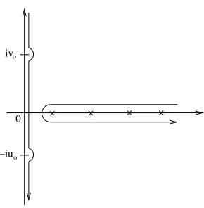
when the regularisation parameter (chosen to have an imaginary part)δ _→0. Now we open up the contour making it run along the imaginary axis avoiding the two poles at z = −iuo, ivo as

in Figure 1. The integral reduces to

I = 1

2π Z ∞

0 ln

1−e−2πxx−uo x+uo

x₋vo

x+vo

d(xcos(δx))− 1

2 Z ∞

0 xcos(δx)dx

− 1

4π Z ∞

0 xe

−iδx 1

x+vo

+ 1

x+uo

dx+J(uo) +J(vo), (5.18)

14

−iu 0 o

[image:22.612.225.370.88.236.2]

o iv

Figure 1: Change of the integration contour forI. Theǫi are denoted by crosses.

where we have separated out the terms J(uo), J(vo) of φwhich have poles on the imaginary axis

and are defined as

J(vo) =−

i 4π

Z

C

ze−δz z−ivo

dz . (5.19)

HereC is a contour consisting of three parts: 0≤ z ≤i(vo−ǫ) forC1, C2 is a small semi-circle

of radiusǫ around ivo and for C3, i(v+ǫ)≤z ≤ ∞. In the limit ǫ→0 we obtain

J(vo) =−

i 4πδ −

vo

4πe

−iδvo_Ei(iδv

o), (5.20)

where Ei(z) is the exponential integral function. The original integral now becomes

I = 1

2π Z ∞

0 ln

1₋e−2πxx−uo x+uo

x−vo

x+vo

d(xcos(δx))

+ 1 2δ2 +

1 4π

i

δ +voe

iδvo_{Γ(0, iδv} o)

− 1

4π i

δ +voe

−iδvo_Ei(iδv o)

+ 1 4π

i

δ +uoe

iδuo_{Γ(0, iδu} o)

− 1

4π i

δ +uoe

−iδuo_Ei(iδu o)

, (5.21)

where Γ(x, y) is the incomplete Gamma function. In the limit δ→0 we find

I _→ 1

2δ2 −

uo+vo

2π ln(iδ)− 1

2π(γ(uo+vo) +uolnuo+volnvo) + 1

2π Z ∞

0 dxln

1₋e−2πxx−uo x+uo

x₋vo

x+vo

. (5.22)

Forvo =uothis expression agrees with the one obtained in [27]. The regularised normal ordering

constant is

c(uo, vo) =

1 2π

Z ∞

0 dxln

1−e−2πxx−uo x+uo

x−vo

x+vo

− ₂1_π(γ(uo+vo) +uolnuo+volnvo). (5.23)

The integral above reproduces the NN and DD normal ordering constants (₋₂₄1) corresponding to uo =vo = 0,∞, respectively. Further, it also reproduces the normal ordering constant of an

ND string (1

48) obtained by taking uo = 0, vo =∞. The terms divergent when the tachyons go

to infinity will cancel with terms coming from the fermion normal ordering constant.15

Returning to the computation of the annulus diagram in the open string channel it is not difficult to compute the partition function for a single boson with boundary conditions (5.4)

Zbosonic(uo, vo) = Tr(e−2πtH bos

o ) = ˜q2c(uo,vo)

∞

Y

n=1

(1₋q˜2ǫn

)−1, (5.24)

with ˜q=e−πt _{and t=π/l.}

A similar analysis has been carried out for the fermions. In the R sector these have the same moding as the bosons; canonically quantised they satisfy the anti-commutation relations

{ψǫn, ψǫn}=δm,−n, (5.25)

and have the Hamiltonian

H_oR= 1 2

∞

X

n=1

ψǫ−nψǫn−c(uo, vo). (5.26)

In the NS sector the moding is different with the ǫr now satisfying

e2i(tan−1

(uo/ǫr)+tan−1(vo/ǫr))

=₋e2πiǫr

. (5.27)

The anti-commutation relations and Hamiltonian are

{ψǫr, ψǫs}=δr,−s, H

NS o =

1 2

∞

X

r=1

ψǫ−rψǫr −cNS(uo, vo), (5.28)

where in the NS sector the regularised normal ordering constant is

cNS(uo, vo) =

1 2π

Z ∞

0 dxln

1 +e−2πxx−uo x+uo

x₋vo

x+vo

− ₂1_π (γ(uo+vo) +uolnuo+volnvo) . (5.29)

The partition function for a NS fermion is

ZNS(uo, vo) = TrNS(e−2πtH NS

o ) = ˜q−2c_NS(uo,vo)

∞

Y

r>0

(1 + ˜q2ǫr

), (5.30)

15

while that of an R fermion is

ZR(uo, vo) = TrR(e−2πtH R

o ) = ˜q−2c(uo,vo)

∞

Y

n=1

(1 + ˜q2ǫn

). (5.31)

It is clear by construction and inspection that the coefficients of ˜q are integral. This is expected of an open string partition function.

Combining equations (5.24), (5.30) and (5.31) the partition function for open strings on a non-BPS D-brane in the presence of background tachyons is

Zopen =

Z ∞

0

dt

2tTrNS-R(e

−2πtHo_{) =} V9

(2π)9

Z ∞

0

dt 2t(2t)

−9/2f37(˜q)g (uo,vo)

3 (˜q)−f27(˜q)g (uo,vo) 2 (˜q)

f7 1(˜q)g

(uo,vo) 1 (˜q)

,

(5.32) whereV9 is the volume of space-time with no background tachyon, and thegfunctions are defined

as

g(1uo,vo)(˜q) = ˜q−2c(uo,vo)

∞

Y

r>0

(1−q˜2ǫn

), g2(uo,vo)(˜q) = ˜q−2c(uo,vo)

∞

Y

r>0

(1 + ˜q2ǫn

), (5.33)

g(3uo,vo)(˜q) = ˜q−2cNS(uo,vo)

∞

Y

r>0

(1 + ˜q2ǫr

), g4(uo,vo)(˜q) = ˜q−2cNS(uo,vo)

∞

Y

r>0

(1−q˜2ǫr

).(5.34)

It is easy to see that in equation (5.32) the terms divergent foruo, vo → ∞in the normal ordering

constants of bosons and fermions cancel.

In this section we have computed the partition function on the annulus by an operator method, slicing time in the periodic direction. In the previous section we used a different operator formal-ism with time running from one boundary of the annulus to the other. Since both approaches compute the same quantity we expect that equations (4.36) and (5.32) should give the same result. For conformal theories this is easily checked using the t → l transformation properties of the fi functions. Unfortunately we do not know the corresponding transformations for the

g_i(uo,vo) and f_i(uc,vc) functions and are, as a result, unable to verify this claim directly.

In the closed string channel discussed in Section 4 the R-R partition function gave a non-zero answer (for uc, vc 6= 0). This can be re-interpreted as the statement that there is a GSO-like

projection acting on open strings in the presence of non-zero tachyons on the boundary. This projection should presumably be defined as a mod 2 number operator for world-sheet fermions just as in the case without background tachyon. This suggests a further contribution to the partition function of interest of the form

Zopen =

Z ∞

0

dt

2tTrNS-R(e

−2πtHo₍₋₁₎F_{) =−} V9

(2π)9

Z ∞

0

dt 2t(2t)

−9/2f47(˜q)g (uo,vo) 4 (˜q)

f7 1(˜q)g

(uo,vo) 1 (˜q)

, (5.35)

6

Conclusion

We have computed the partition function in the supersymmetric boundary sigma model on the annulus for the case of the exactly solvable linear tachyon profile. We showed how the one and the same answer can be achieved by means of different techniques: the Green’s function method and the boundary state formalism, justifying thereby the latter for the case of non-conformal boundary deformations. An interesting feature of our results is that the R-R sector provides a non-trivial contribution to the partition function. If the interpretation of the annulus partition function as a one-loop correction to the space-time effective action Seff is correct one

may determine the corresponding change inSeff. Taking the tachyon profile to be the same on the

two boundaries one may expand the partition function around smalluand interpret it as coming from an effective space-time action for the tachyon field T. In the R-R sector only zero-modes contribute to the leading order in u-expansion and one finds

S_{eff, R-R}1−loop _∼ Z

d10x Z 1

0

da a K(a)e

−1 4(1+a)T

2

[∂µT ∂µT+Fµν2 ∂µT ∂νT−

1 2∂µT ∂

µ_{T F}

νρFνρ+. . .], (6.36)

where we have indicated by dots the higher derivative terms and the mixing between the tachyon and the gauge field comes from the zero-modes as discussed in Section 3.3. In the above

K(a) = f

8 2(a)

f8 1(a)

. (6.37)

Thus, the R-R sector contributes only to the derivative terms and not to the tree level potential. Similarly expanding the NS-NS partition function inu one finds its contribution to the effective action as

S_{eff, NS-NS}1−loop ∼

Z d10x

Z 1

0

da a K(a)e

−1 4(1+a)T

2

[1 +b(a)∂µT ∂µT +. . .]. (6.38)

Hereb(a) is the next-to-leading term in theu-expansion of the NS-NS partition function. The integral overadiverges due to thea _→1 behaviour of the integrand. This arises from the open string tachyon and should be subtracted in a manner compatible with open/closed string duality. It is desirable to find such a subtraction scheme. This divergence indicates the instability of theT = 0 vacuum [39, 27]. In obtaining the partition function in the closed string channel we have summed over the spin structures, thus removing the closed string tachyon. This manifests itself in the fact that the a integral above has no linear divergences for a → 0. However, there is a logarithmic divergence in the a → 0 limit corresponding to a massless exchange. It is an interesting question whether this divergence (in the case of the superstring) can be treated using a Fischler-Susskind type mechanism [40].

the normal ordering constant of the open string Hamiltonian that depends on the tachyon profile in a non-trivial way. Clearly the normal ordering constant is divergent and usually one picks up a subtraction scheme to define a finite quantity c. We discussed such a scheme (generalising the one in [27]) accounting for two different boundary tachyons. The part of cthat is finite when u orv goes to infinity reproduces the normal ordering constants for the NN,DD and ND cases.

Note added. When our work was completed an interesting paper [41] appeared where the

some issues related to the construction of the loop corrected tachyon potential were discussed.

Acknowledgements

We would like to thank M. Bianchi, M.B. Green, I. Runkel, C. Schweigert, P. Vanhove and particularly S. Silva for many helpful conversations and useful insights. S. Frolov has provided many valuable comments on the manuscript. We are especially grateful to S. Theisen for initially collaborating on the project, for reading the manuscript and for sharing his insights. G.A. was supported by the DFG and in part by RFBI grant N99-01-00166 and by INTAS-99-1782. We are supported by the European Commission RTN programme HPRN-CT-2000-00131 in which we are associated to U. Bonn. A.P. also acknowledges support from GIF, the German-Israeli foundation for Scientific Research under grant number I-522-010.07/97.

A

Derivation of Green’s functions and the partition

func-tion

In the Appendix we present the explicit expressions for the various Green’s functions. We dis-cuss in some detail the bosonic boundary conditions, their relation to Gauss’s theorem and the transposition properties of the Green’s function. Finally, we briefly outline how to obtain the partition function from the Green’s function.

A.1

Green’s functions

A.1.1 The bosonic sector

Consider the more general boundary conditions for the bosonic Green’s function

(z∂z+ ¯z∂z¯)G(z, w) +uG(z, w) +F(z∂z−z∂¯ z¯)G(z, w) = D, |z|= 1,

where D and E are yet unknown matrices that may depend on the fields. Since Gµν(z, w) =

hXµ(z)Xν(w)i the Green’s function must satisfy

Gµν(z, w) =Gνµ(w, z). (A.2)

To find the Green’s function corresponding to the boundary conditions (A.1) we make the ansatz

G(z, w) =Gf(z, w) +A+Bln|z|2ln|w|2+Cln|z|2+CT ln|w|2+

X

k∈Z\{0}

(αk(w)zk+ ¯αk(w)¯zk),

(A.3) where Gf(z, w) = −ln|z−w|2 is the fiducial Green’s function, obeying (α′ = 2)

− 1

2π∂z∂¯zGf(z, w) =δ

(2)_{(z, w). (A.4)}

Moreover we require that A, B and C are real matrices, satisfying

A=AT, B =BT. (A.5)

The derivation of the oscillators is straightforward and one finds

αk =

1 k

1₋a2kSk(u, F)Sk(av, L)

−1

Sk(u, F)

¯

wk+a2kw−kSk(av, L)

,

α−k =

a2k

k

1₋a2kS_kT(av, L)S_kT(u, F)−1S_kT(av, L)w¯−k+wkS_kT(u, F),

˜ αk =

1 k

1₋a2kS_kT(u, F)S_kT(av, L)−1S_kT(u, F)wk+a2kw¯−kS_kT(av, L) ,

˜ α−k =

a2k

k

1₋a2kSk(av, L)Sk(u, F)

−1

Sk(av, L)

w−k+ ¯wkSk(u, F)

. (A.6)

It is easy to see that the oscillator dependent parts of the Green’s function indeed satisfy (A.2). For the zero-modes we find the conditions

−2 + 2C+uA−D+ (2B+uCT) ln|w|2 _{= 0, |z|= 1,(A.7)}

−2C+av(A+ 2Clna)−E+ (−2B−av+ 2avBlna+avCT) ln|w|2 _{= 0, |z|=a .(A.8)}

Taking into account (A.5), the cancellation of the ln_|w_|2 _{dependent terms in (A.7) and (A.8)}

requires that

B =−1

2Cu and uC

T _{=Cu (A.9)}

and C is explicitly found to be

From this expression one may check that CT _{indeed satisfies the constraint uC}T _{= Cu.}

Solv-ing (A.7) one finds

uA= (2(1−C) +D), uDT =Du (A.11)

and (A.8) implies

Eu=avDT . (A.12)

Thus, the matrices D and E are related by (A.12) but not completely fixed by the boundary conditions. Since a non-vanishing D only results in a change of the overall normalisation of the (bosonic) partition function it is convenient to choose D= 0 =E. Then A is explicitly given by

A= 2(1₋avlna)(u+av₋auvlna)−1, (A.13) modulo elements in the kernel of u which we suppress for the same reasons as a non-vanishing D.

As a final check, we prove that Gauss’s theorem is satisfied for any D. Since the Green’s function satisfies

✷G(σ1, σ2) =−4πδ(2)(σ1, σ2) (A.14)

together with the boundary conditions (A.1), Gauss’s theorem requires

−4π= Z

∂Σ∂rGds=−u

Z

|z|=1dφ G(z, w)−av

Z

|z|=adφ G(z, w) + 2π(D+E). (A.15)

Only the integrals over the zero-modes will be non-vanishing and, therefore we confirm that

0 = 4π−2π(uA+avA+ 2avClna−D−E+ ln|w|2_(uCT _{−av+ 2avBlna+avC}T_{)). (A.16)}

A.1.2 The NS-NS sector

Here we present the explicit expressions for the oscillators of the various Green’s functions in the NS-NS sector. For example, theG++ oscillators are

ψr(w) = iηηa˜ 2r

1₋ηηa˜ 2rSr(u, F)Sr(av, L)

−1

Sr(u, F)Sr(av, L)w−r,

ψ−r(w) = −iηηa˜ 2r

1₋ηηa˜ 2rS_rT(av, L)S_rT(u, F)−1S_rT(av, L)S_rT(u, F)wr. (A.17) Similarly

˜

ψr( ¯w) = iηηa˜ 2r

1₋ηηa˜ 2rS_rT(u, F)S_rT(av, L)−1S_rT(u, F)S_rT(av, L) ¯w−r, ˜

ψ−r( ¯w) = −iηηa˜ 2r

1₋ηηa˜ 2rSr(av, L)Sr(u, F)

−1

Sr(av, L)Sr(u, F) ¯wr, (A.18)

ar( ¯w) = η

1₋ηηa˜ 2rSr(u, F)Sr(av, L)

−1

Sr(u, F) ¯wr,

a−r( ¯w) = −ηa˜ 2r

and

br(w) = −η

1−ηηa˜ 2rS_rT(u, F)S_rT(av, L)−1S_rT(u, F)wr, b−r(w) = ˜ηa2r

1−ηηa˜ 2rSr(av, L)Sr(u, F)

−1

Sr(av, L)w−r. (A.20)

A.1.3 The R-R sector

For the non-zero modes the oscillators are exactly the same as in the NS-NS sector, the only difference being that now r is an integer.

A.2

The partition function

In this sub-section we outline the derivation of the partition function in the closed channel following a technique used in [15]. For simplicity we restrict ourselves to the bosonic contribution, the derivation of the fermionic parts proceeds exactly along the same lines.

Differentiation of the (bosonic part of the) boundary action with respect to the couplings u and v results in the differential equations

∂lnZ

∂uµν = −

1 8π

Z 2π

0 dφhXµ(φ)Xν(φ)i=−

1 8π

Z 2π

0 dφ Gµν(e

iφ_{, e}iφ_),

∂lnZ

∂vµν = −

1 8π

Z 2π

0 dφ aGµν(ae

iφ_{, ae}iφ_{) (A.21)}

and similar equations when differentiating with respect to F and L. Using the result for the bosonic Green’s function it is not difficult to verify that the solution to these equations (up to the normalization) is

Zbos = det(u+av−auvlna)−1/2

∞

Y

k=1

det(1 +u/k+F)−1det(1 +av/k+L)−1

× det1₋a2kSk(u, F)Sk(v, L)

−1

. (A.22)

Z also satisfies the equations obtained by differentiating with respect toFµν andLµν. In principle

there may be an overall dependence on the modulus a in the partition function that could not be fixed by the previous considerations. However, one can also derive an equation for ∂lnZ

∂a by

looking at the change of the action under variations of the modulus [33]. Following [33] this equation reads

∂alnZ = −h∂aSbulki − h∂aSbndyi

= 1

2π a 1₋a2

Z

Σd 2_z 1

¯

z2hTzzi+

1 z2hTz¯z¯i

− ₈1_π

Z 2π

0 dφ vµνG

Using the explicit expression for the bosonic Green’s function and

hTzz(z)i=−

1 2wlim→z

"

∂z∂wGµµ(z, w) +

10 (z−w)2

#

(A.24)

and similarly for_hTz¯z¯i we find that∂alnZ integrates to (3.5), so that there is no further

depen-dence on the modulus.

References

[1] A. Sen,Descent relations among bosonic D-branes, Int. J. Mod. Phys. A14(1999) 4061 hep-th/9902105; Stable non-BPS bound states of BPS D-branes, JHEP 9808(1998) 010, hep-th/9805019; Tachyon condensation on the brane antibrane system, JHEP 9808(1998) 012, hep-th/9805170; Non-BPS states and branes in string theory, hep-th/9904207; Supersym-metric world-volume action for non-BPS D-branes, JHEP9910(1999) 008,hep-th/9909062;

Universality of the tachyon potential, JHEP 9912(1999) 027, hep-th/9911116.

[2] E. Witten,D-branes and K-theory, JHEP9812(1998) 019,hep-th/9810188.

[3] O. Bergman, M.R. Gaberdiel, Stable non-BPS D-particles, Phys. Lett. B441, 133 (1998), hep-th/9806155.

[4] E. Witten,Non-commutative geometry and string field theory, Nucl. Phys.B268(1986) 253.

[5] V. A. Kostelecky and S. Samuel, On a non-perturbative vacuum for the open bosonic string, Nucl. Phys.B336(1990) 263; A. Sen and B. Zwiebach,Tachyon condensation in string field theory, JHEP 0003(2000) 002 hep-th/9912249; N. Moeller and W. Taylor, Level truncation and the tachyon in open bosonic string field theory, Nucl. Phys. B583 (2000) 105 hep-th/0002237;R. de Mello Koch, A. Jevicki, M. Mihailescu and R. Tatar,Lumps and p-branes in open string field theory, Phys. Lett.482B(2000) 249,hep-th/0003031;N. Moeller, A. Sen and B. Zwiebach, D-branes as tachyon lumps in string field theory, JHEP 0008(2000) 039, hep-th/0005036;N. Berkovits,The tachyon potential in open Neveu-Schwarz string field the-ory, JHEP0004(2000) 022,hep-th/0001084;N. Berkovits, A. Sen and B. Zwiebach,Tachyon condensation in superstring field theory, Nucl. Phys. B587 (2000) 147, hep-th/0002211; I. Y. Aref’eva, A. S. Koshelev, D. M. Belov and P. B. Medvedev, Tachyon condensation in cubic superstring field theory, hep-th/0011117.

[6] J. A. Harvey, D. Kutasov and E. J. Martinec,On the relevance of tachyons,hep-th/0003101.

[8] A. A. Gerasimov and S. L. Shatashvili,On exact tachyon potential in open string field theory, JHEP 0010(2000) 034, hep-th/0009103.

[9] D. Kutasov, M. Marino and G. Moore,Some exact results on tachyon condensation in string field theory, JHEP 0010(2000) 045, hep-th/0009148.

[10] D. Ghoshal and A. Sen, Normalization of the Background Independent Open String Field Theory Action, JHEP 0011(2000) 021, hep-th/0009191.

[11] D. Kutasov, M. Marino and G. Moore, Remarks on tachyon condensation in superstring field theory, hep-th/0010108.

[12] O. Andreev,Some computations of partition functions and tachyon potentials in background independent off-shell string theory, Nucl. Phys. B598(2001) 151, hep-th/0010218.

[13] A.A. Gerasimov and S.L. Shatashvili,Stringy Higgs mechanism and the fate of open strings, JHEP 0101(2001) 019, hep-th/0011009.

[14] P. Kraus and F. Larsen,Boundary String Field Theory of the DDbar System, Phys.Rev.D63

(2001) 106004, hep-th/0012198; T. Takayanagi, S. Terashima, T. Uesugi, Brane-Antibrane action from boundary string field theory, JHEP0103(2001) 019,hep-th/0012210.

[15] E. Witten,On background-independent open string field theory, Phys. Rev.D46(1992) 5467, hep-th/9208027; Some computations in the background-independent off-shell string theory, Phys. Rev. D47(1993) 3405, hep-th/9210065.

[16] S. Shatashvili, Comment on the background independent open string theory, Phys. Lett.

311B (1993) 83, hep-th/9303143; On the problems with background independence in string theory,hep-th/9311177.

[17] G. Arutyunov, S. Frolov, S. Theisen and A. A. Tseytlin,Tachyon condensation and univer-sality of DBI action, JHEP0102(2001) 002, hep-th/0012080.

[18] A. Tseytlin, Sigma model approach to string theory effective actions with tachyons, hep-th/0011033.

[19] M. Marino,On the BV Formulation of Boundary Superstring Field Theory,hep-th/0103089.

[20] V. Niarchos and N. Prezas, Boundary Superstring Field Theory,hep-th/0103102.

1257; O. D. Andreev and A. A. Tseytlin, Partition function representation for the open superstring action: cancellation of Mobius infinities and derivative corrections to Born-Infeld Lagrangian, Nucl. Phys. B311 (1988) 205;

[22] S. Frolov, On off-shell structure of open string sigma model, hep-th/0104042.

[23] R. Rashkov, K. S. Viswanathan and Y. Yang, Background independent open string field theory with constant B field on the annulus,hep-th/0101207.

[24] T. Suyama,Tachyon condensation and spectrum of strings on D-branes,hep-th/0102192.

[25] K. S. Viswanathan and Y. Yang,Tachyon condensation and background independent super-string field theory, hep-th/0104099.

[26] M. Alishahiha,One-loop correction of the tachyon action in boundary superstring field theory, hep-th/0104164.

[27] K. Bardakci and A. Konechny, Tachyon condensation in boundary string field theory at one loop, hep-th/0105098.

[28] A.M. Polyakov,Quantum Geometry of Bosonic Strings, Phys. Lett. 103B (1981) 207.

[29] C.G. Callan, jr., C. Lovelace, C.R. Nappi and S.A. Yost, Adding holes and crosscaps to the superstring, Nucl. Phys. B293(1987) 83.

[30] J. Polchinski and Y. Cai,Consistency of open superstring theories, Nucl. Phys.B296(1988) 91.

[31] S. P. de Alwis, Boundary string field theory, the boundary state formalism and D-brane tension, Phys. Lett. 505B(2001) 215, hep-th/0101200.

[32] C.G. Callan, jr., C. Lovelace, C.R. Nappi and S.A. Yost, Loop corrections to superstring equations of motion, Nucl. Phys. B308 (1988) 221.

[33] A. Abouelsaood, C.G. Callan, C.R. Nappi, S.A. Yost, Open strings in background gauge fields, Nucl. Phys. B280(1987) 599.

[34] M. Bill´o, P. Di Vecchia, M. Frau, A. Lerda, I. Pesando, R. Russo, S. Sciuto, Microscopic string analysis of the D0-D8 brane system and dual R-R states, Nucl. Phys. B526 (1998) 199, hep-th/9802088.

[36] B. Stefa´nski, jr.,Gravitational couplings of D-branes and O-planes, Nucl. Phys.B548(1999) 275, hep-th/9812088.

[37] J.F. Morales, C.A. Scrucca, M. Serone, Anomalous couplings for D-branes and O-planes, Nucl. Phys. B552 (1999) 291,hep-th/9812071.

[38] M. Bill´o, B. Craps, F. Roose, Ramond-Ramond couplings of non-BPS D-branes, JHEP

9906(1999) 033, hep-th/9905157.

[39] N. Marcus, Unitarity and regularized divergences in string amplitudes, Phys. Lett. 219B

(1989) 265.

[40] W. Fischler, L. Susskind, Dilaton tadpoles, string condensates and scale invariance, Phys. Lett. 171B(1986) 383.