Pressure transients in a ruptured gas pipeline with friction and thermal effects included

(1)

City, University of London Institutional Repository

Citation

:

Tiley, C.H. (1989). Pressure transients in a ruptured gas pipeline with friction and thermal effects included. (Unpublished Doctoral thesis, City University)

This is the draft version of the paper.

This version of the publication may differ from the final published

version.

Permanent repository link:

http://openaccess.city.ac.uk/17971/

Link to published version

:

Copyright and reuse:

City Research Online aims to make research

outputs of City, University of London available to a wider audience.

Copyright and Moral Rights remain with the author(s) and/or copyright

holders. URLs from City Research Online may be freely distributed and

linked to.

(2)

CITY UNIVERSITY

DEPARTMENT OF MECHANICAL ENGINEERING &: AERONAUTICS

PRESSURE TRANSIENTS IN A RUPTURED GAS PIPELINE WITH FRICTION AND THERMAL EFFECTS INCLUDED

by-C.H. TILEY

A Dissertation submitted to City- University for the Degree of Doctor of Philosophy-in Mechanical EngPhilosophy-ineerPhilosophy-ing

(3)

IMAGING SERVICES NORTH

Boston Spa, Wetherby

West Yorkshire, LS23 7BQ www.bl.uk

TEXT CUT OFF IN THE

(4)

LIST OF CO~~~S

LIST OF FIGURES ACKNOWLEDGEMEl\'TS

ABSTRACT

NCY.1ENCLATliRE

LIST OF CONTENTS

CHAPTER 1: INTRODUCTION

CRf\PTER 2: THEDRErICAL DE\'ELOP!'1E!\"T OF THE BASIC mUATIONS

2.1. Introduction

2.2. Conservation of Mass

2.3. Conservation of Linear Homentum 2.4. Conservation of Ener~'

2.5. Basic Equations in terms of Pressure, Velocity, and Temperature

2.6. The Friction Term 2. i. The Heat Transfer Term 2.8. The Compressibility Factor

CHAPTER 3: RE\'IE;\\7 OF THE METHODS OF SOLUTIOK

3.1. Introduction

3.2. The Method of Characteristics 3.3. EA-plici t Finite Difference ~lethods 3.4. Implicit Finite Difference Methods

3.~. Solution of a Riemann Problem - Random Choice and Flux Difference Splitting Schemes

3.6. Finite Element Analysis 3.7. Discussion

CHAPTER 4: SOLl~ION OF THE CHARACTERISTIC mUATIOKS FOR

1 7 8 9 10 17 Ii' 18 19 20 22 23 26 30 35 ' ) -,,0 35 ~8 55 62 68 71

A LIl\o·EBIlli.tJ{ SITUATION 75

4.1. Introduction 75

4.2. General Solution for Internal Points 77 4.3. Specific Solutions for Various Grid ?oint

Configurations 82

4.3.1. Internal point ld th equi -distant adjacent

grid points 82

(5)

4.4. Cpstream Boundary Condition 4.3. Downstream BOlmdary Condition 4.6. Break BOlmdary Condi tion

CHAPTER 5: CDHPUTrn ~10DEL

5.1. Introduction

5.2. Transient Analysis Program 5.2.1. Main program

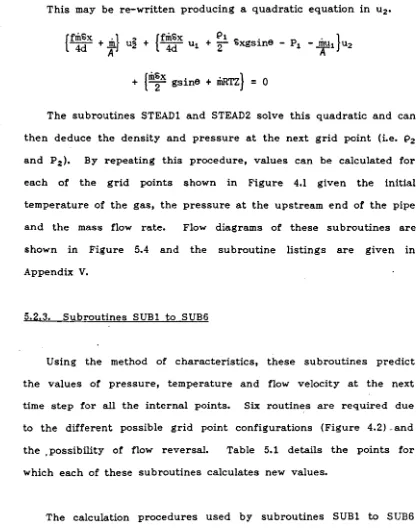
5.2.2. Subroutines STEAD1 and STEAD2 5.2.3. Subroutines SUB1 to SL~6 5.2.4. Subroutines BREAK1 to BREAK4 5.2.5. Subroutines Sl~l~ and DOWN1 5.3. Graphics Program

CHAPTER 6: EXPERIMENTAL DATA

6.1. Introduction

6.2.

Review of Laboratory K~~riments

6.3. Review of Full Size Tests

6.4.

Selection of Test Data

6.5. Preparation of the Data

6.5.1. Preparation of gas data

6.3.2 •.

Preparation of system data

93 96 103 103 104 104 107 109

111

116 123 IN 124 123 128 134 140

HO

142

CHAPTER 7: RESULTS l-! i

7.1. Introduction 147

7.2. Groves' Shock Tube Results 148

7.3. British Gas Shock Tube Results 152

7.4. Foothills Pipelines (Yukon) Ltd. Full Size Result.s 166

CHAPTER 8:

DISCUSSION 180

8.1. General Discussion of Results 180

8.1.1.

8.1.2.

8.1.3.

Groves' Shock Tube Results British Gas Shock Tube Results

Foothills Pipelines (Yukon) Ltd. Full Size Results

8.2. Discussion of Errors

CK~ 9: CONCLUSIONS

(6)

CHAPTER 10: 10.l. 10.2. 10.3. 10.4.

APPB-J1HCES :

ruRTHER WORK

Investigation of the Wavespeed Error Further Testing of the Present Model

Improvement of the Stability of the Solution Further Refinement of the Model

I. Derivation of the Basic Partial Differential

Equations, with Pressure, Temperature and Velocity as the Dependent Variables.

II. Friction Factor Relationships

Ill. Implementation of Taylor's Theorem for Various Grid Points

IV. Derivation of the Particle Velocity of a Rarefaction Wave

V. Program Listings

VI. Preparation of Gas Data

REFERENCES

19i 197 198 198 198

200

206

212

218

225

293

(7)

1.1. 1. 2.

2.1-2.2. 2.3. 2.4.

2.5.

2.6. 3.1.

3.2.

3.3. 3.4. 3.0. 3.6. 3.7. 3.8. 3.9.

3.10.

3.11.

-1:.1., 4.2. 4.3. 4.4.

4.5.

4.6.

LIST OF FIGURES

Typical Phase Diagram for Natural Gas

Pipe Failure Distribution for Natural Gas Lines

Control Volume Illustrating the Conservation of Mass Control Volume Illustrating the Conservation of Linear Momentum

Control Volume Illustrating the Conservation of Energy Heat Transfer into the Pipe

Heat Transfer into the Pipe - Simplified Hodel Generalized Compressibility Factor Chart

Two-Dimensional Natural Grid of Characteristics Linear Characteristics on an x-t plane

Characteristics on a Rectangular Grid for Two Dependent Variables

Characteristics for Three Dependent Variables on a Rectangular Grid

Possible Problem Areas wnen Using the Mesh ~lethod of Characteristics

The Finite Difference Grid Illustrating a Two-step Method

An

x~t Grid for Illustrating Implicit FInite Difference

~1ethods

Grid Points used in Variol~ Finite Difference Methods Weighted Finite Difference Approximations

Elemental Section for Flux Difference Splitting Discontinuity Between Two Half Sections

Grid Size Variation for Modelling a Linebreak Different Internal Grid Point Configurations Effect of Flow Reversal on the Characteristics Grid Point Linking Two Different Grid Sizes Downstream Boundary Condition

Pressure Drop at the Break

4

(8)

---~---5.1. 5.2. 5.3. 5.-1:. 5.5a. 5.5b.

5.6.

5.7.

5.8a. 5.8b. 5.8c. 5.9a. 5.9b. 6.1. 6.2. 6.3. 7.1. 7.2. .7.3. 7.4.

7.5.

7.6.

7.7.

7.8. 7.9. 7.10. 7.11. 7.12. 7.13.

7.14.

7.15.

Data Preparation Sheet

Marching Process of Calculation

Linear Momentum Equation for Steady One-dimensional Pipe Flow

Flow Diagrams for STEADl and STEAD2 Flow Diagrams for SUBl, SUB2, and SliB5 Flow Diagrams for StiB3, SUB4, and SL'B6 Break Point Prior to Rupture

Break Point After Rupture Flow Diagram for BREAKl Flow Diagram for BREAK3 Flow Diagram for BREAK4

Flow Diagram for SL~L~ Flow Diagram for DOw~l

Shock Tube Used by Groves et al. British Gas Shock Tube

Test Sections Used by Foothills Pipelines (Yukon) Ltd.

=

0.03 P

x

=

0.0027) P x t Graph for British Gas Shock Tube Test 7} (f

=

0.03 P

x

₌

0.0027) 7.16. P x t Graph for Foothills Test Results NABTFl (West)

7.17. P x t Graph for Foothills Test Results NABTFl (East) 7.18. P x w Graph for Foothills Test Results NABTFl

(9)

7.21. P

x W Graph for Foothills Test Results

NABTF3

7.22. P

x t Graph for Foothills Test Results NABTF~ IWest)

7.23. P

x W Graph for Foothills Test Results NABTF~ lEast)

7.2~. p x

w

Graph for Foothills Test Results NABTF~

7.25. P

x t Graph for Foothills Test Results

NABTF5

(West)

7.26. P

x t Graph for Foothills Test Results

NABTF5

(East

7.27.

P x W Graph for Foothills Test Results

NABTF5

8.1. Approximation of dp/dp on a Finite Grid 8.2. Pipe Rupture in a Full Size Pipe

8.3. Variation of the Specific Heat of ~lethane

A.l. Model of Fluid Movement in a Tube

A.2. Coefficient Charts for use in the Method of Grieves and Thodos

6

(10)

~---ACKNOWLEDGEMENTS

This project was conducted with the sponsorship of the Science

& Engineering Research Council.

Special thanks go to my supervisor, Professor A.R.D. Thorley, for all his help and advice during the course of this project and for the encouragement he has given me throughout the work • .

.

I would also like to thank other members of staff in the Department of Mechanical Engineering & Aeronautics at City University for their support.

Thanks are also due to Professor

v;

Price and staff in the Computing Department at City University for their help with the numerical analysis and programming involved in this project.

I would also like to thank David Jones from British Gas (Engineering Research Station) and Brian Rothwell from Foothills Pipelines (Yukon) Ltd., for their help and for supplying me ,dth some experimental data without which I could not have successfully tested my theoretical model.

(11)

ABSTRACT

A theoretical model has been developed which can simulate a linebreak occurring in a gas pipeline. By assuming one-dimensional homogeneous gas flow and neglecting minor losses and changes in cross-sectional area of the pipe, three simultaneous non-linear partial differential equations were derived from first principles which mathematically model pressure transients in a non-perfect gas. A constant value steady-flow friction factor was used to calculate the frictional losses which was considered to be a reasonable approach since it would not be possible to account for all the variations in friction. The heat transfer into the pipe was accounted for using a constant value Stanton Number approach which again was an acceptable approximation considering the comparatively small effect that heat transfer has on the pressure transients.

The equations were converted to ordinary differential equations using the Method of Characteristics and these were then solved numerically using a Taylor expansion. A novel feature of this project was the incorporation of a reduced grid size in the vicinity of the break allowing closer monitoring of the expansion waves in this area. Also included was a means of modelling flow reversal in the pipe which enabled situations with a non-zero initial flow rate to be simulated.

A computer code solving the mathematical model was written in Fortran 77 for use on a Gould PN9005 mainframe computer. Both tabular and graphical output were produced which could then be compared with available experimental data.

The ~xperimental data that was selected for validation of the theoretical model included shock tube test results and some full size tests. Reasonable agreement was obtained between the theoretical and experimental results and any possible error sources were investigated.

(12)

NOMENCLATURE

The s}1mbols used in this text have the following meanings, except where they have been otherwise specifically defined:

SYmbol

A

d e

Cross-sectional area of pipe Isentropic wavespeed

Specific heat at constant preSSl~e Specific heat at constant vohune Diameter of pipe

Specific internal energy f Darcy friction factor

g h

~}

P

Acceleration due to gravi t~' Specific enthalpy

Rectangular coordinates used in explicit finite difference methods

Pressure

Pr Prandtl number

Q

R

Heat transfer rate per unit volume Specific gas constant

Re Reynolcts number

s St T t u

w

Specific entropy Stanton number

Temperature of the gas Time

Velocity of the gas

Frictional force per unit length of pipe Distance along the pipe

x Thermodynamic quality or dr~~ess fraction z Gas Compressibility factor

Greek SYmbols

L'nits

m

2

m/s J/kg K J/kg

K

m J/kg m/s2 J/kg Pa <3 J/m s

J/kg

J/kg K

K

s m/s N/m

m

e Angle of inclination of pipe to the horizontal Had

P Mean density of the gas kg/m<3

o

Heat flow into the pipe per unit length of pipe

and per uni t time J

/IDS

w actual wave propagation speed selective

(13)

CHAPTER 1 INTRODUCTION

Ever since the first gas pipelines of the Western World were laid in Philadelphia (1796), Genova (1802), and Fredonia (1821), the demand for gas as an energy source has been growing worldwide. Gas is now considered to be one of the most valuable raw materials due to its high calorific value and so safe and efficient transportation is of prime importance.

Up until the mid 1960's, this country was using town gas which was manufactured in gas-making plants in the towns and then distributed locally at relatively low pressures. Originally i in the 1920's and 1930's, the pipes for this gas distribution were made from cast iron but these were irregular in shape and thickness and by

(,~,".r.~--;T""'-:--.-f"",'.'.

the mid. twentieth:i _{century steel pipes were being used.}

' .... _.:~.~ .... _~..tc.!.. ..:,...--!....::.:z.-"

With the advent of natural gas as an energy resource in this country, longer distance pipelines became necessary, and in 1964 the first natural gas .steel pipeline in the U.K. was installed, connecting

~he liquefied natural gas import terminal at Canvey Island with the Midlands. Following the discovery of natural gas in the U.K. sector of the North Sea, long distance deep-water lines were built, for example, the 354 km long, 350 mm diameter pipeline installed in 1973/4 between the northern North Sea (Ekofisk platform) and Teeside.

On these early long distance gas transmission systems, compression of the gas (necessary in order to overcome the

(14)

expansion of the gas due to friction) was by reciprocatin g compressors driven by gas or diesel engines. Although machines of this type could compress gas over a wide range of pressures and flows, there has been an almost complete switch to centrifugal machines driven by gas turbines. These are more suitable for handling large volumes of gas although they will only deliver over a restricted combination of pressure and flow.

Today, gas supplies 20% of the primary energy demand in Britain, most of this coming from the North Sea. The offshore gas is landed and treated by North Sea operating companies at coastal terminals and is then fed into the national grid. The national grid consists of three main

sections:-i) National transmission system - approximately 5000 km of pipes with diameters of up to 1050 mm, operating at pressures up to 70 bar.

ii) Regional distribution systems - approximately 12000 km of smaller diameter pipes (minimum diameter

=

100 mm), operating at pressures of 7 bar upwards.

iii) Local service systems - small diameter pipe operating at low pressures.

(15)

network. In total, the overall length of natural gas pipelines makes up 70% of all the world's pipelines.

However, there are some problems involved with natural gas transportation by pipeline. Although containing a high proportion of methane, it is also rich in heavier gas components such as butane and pentane. Since these heavier components are liquid at normal temperatures and pressures (between 0 and 20' C and up to approximately 100 bar) the natural gas. exists as a two-phase mixture under those conditions as shown in Figure 1.1.

QJ

120

'

-

:::J,-"'re

"'..0

100 QJ-LIQUID

'-0...

DENSE PHASE

cricondenbar

.1..;;::.

-BO

60

40 _LI

_{QUID -}

_VA

_POUR

-100 -00 -60 -40 -20 0

20 40 Temperature

(0C)

Figure 1.1. Typical Phase Diagram for Natural_ Gas

Two-phase flow in long distance pipelines is undesirable. The denser liquid phase tends to collect at the bottom of the pipe and since its flow velocity is less than that of the gas phase, the capacity of the pipe is reduced. Also, as the faster gas phase passes over the liquid phase, \\iaves are created which can eventually build up across the entire cross-section of the pipe creating slug flow. This highly non-steady flow, accentuated by any changes in

(16)

elevation of the pipe, should be avoided since the slugs of liquid being propelled along the pipe can cause serious damage to pipe fittings and equipment. One way of avoiding this situation is by regularly pigging the line carrying the two-phase mixtures. This, however, incorporates substantial costs in the setting-up and operation of the pigging stations.

A more cost effective solution is to transport the natural gas at very high pressures in a single phase, known as the dense phase. The dense phase is defined by the critical point and the cricondenbar (the highest pressure at which separated liquid and vapour phases can co-exist). This is illustrated in Figure 1.1.. It

has been found that at these high pressures the gas mixture follows the same equations as single phase gas flow at lower pressure (Oranje, Graaff and Fagerland [1985]).

With these dense phase gases being transported in high pressure, large diameter trunk pipelines, the transient behaviour is of greater significance and economic concern than with the previous gas distribution network. A transient analysis is required to accurately forecast the possibility of the liquid phase appearing as well as improving the overall reliability of the system and optimising the operating conditions.

(17)

changes in demand, for example, on a daily cycle. A slow transient analysis is mainly concerned with the packing and unpacking of gas in the pipeline. There has been a considerable amount of research directed towards this type of transient and various computer software packages are available which model this type of flow (for example, Bender (1979J, Goldfinch [1984], Guy [1967], and Heath and Blunt [1969]).

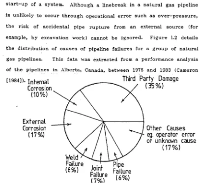
This is less true of rapid transients which are those caused by a linebreak (pipe rupture), compressor failure, or rapid shut-down or start-up of a system. Although a line break in a natural gas pipeline is unlikely to occur through operational error such as over-pressure, the risk of accidental pipe rupture from an external source (for example, by excavation work) cannot be ignored. Figure 1.2 details the distribution of causes of pipeline failures for a group of natural gas pipelines. This data was extracted from a performance analysis of the pipelines in Alberta, Canada, between 1975 and 1983 (Cameron [1984]).

Internal

Corrosion

(10%)

External

Corrosion

(17%)

Joint

Failure

(7%)

Third Party Damage

(35%)

Other Causes

ego

cperator error

or unknown cause

(17%)

Figure 1.2. Pipe Failure Distribution for Natural Gas Lines

14

[image:17.513.60.465.307.679.2]

(18)

~---"---~---Some authors argue that since the rapid transients caused by an event such as a line break are rapidly attenuated in gas pipelines, they are of little significance compared with the slower transients caused by the packing and unpacking of the gas. However, the detection of a linebreak can be important both from an economic and a safety point of view. A transient analysis is therefore required which will simulate the conditions at the break and in the section of pipe either side of the break so that the potential hazard arising from such a situation may be assessed. The analysis could also provide a basis for the design of automatic valve closing devices and alarms which would minimise the effects of such an accident.

Although there have been a few computer programs developed which will model rapid gas transients (for example, Issa [1970], and van Dean and Reintsema [1983]), it was found, on examination, that these models had their limitations. One major consideration was that since the focus of this investigation was on high pressure, dense phase gas transportation, it was essential that the model could simulate the behaviour of a non-perfect gas following a line break. The inclusion of realistic estimates of the effects of friction and heat transfer in the model was also a requisite of the program. Therefore it was decided to develop a new computer code which would incorporate these features.

(19)

The computer model that was developed featured a reduced grid size in the vicinity of the break in order to capture in detail the expansion waves created without excessively prolonging the computer run time. It also successfully simulated the flow reversal that would occur in the section of pipe downstream of the break.

Theoretical results produced from this program have been compared with experimental data obtained from various external sources. These were carefully selected to include realistic data from pipelines generally of the same size and containing gaseous fluids similar to those found in typical dense phase gas transmission lines, as well as data from some fundamental shock tube tests. Reasonable agreement was obtained between the theoretical and experimental results.

(20)

CHAPTER 2

THEORETICAL DEVELOPMENT OF THE BASIC EQUATIONS

2.1. INTRODUCTION

Basic equations describing homogeneous turbulent gas flow in a pipeline were derived from first principles by defining a control volume of fixed location or translating with uniform velocity (see Figure

2.1).

This control volume was of length dx and had a cross-sectional area equal to that of the pipeline. It was assumed that the flow was geometrically one-dimensional, i.e. that all fluid properties were uniform over each cross-section of the pipe. This assumption was examined in detail by Goldwater and Fincham [1980], but briefly it may be stated that for high Reynolds number flows (as in gas transmission lines), the one-dimensional approximation has been shown to be very good for steady and slowly varying flows. There could, however, be some slight deviations when considering large~ rapid disturbances.

(21)

2.2. CONSERVATION OF MASS

The net rate of mass now out of the control volume is equal to the rate of decrease of mass within the control volume. Referring to Figure 2.1

below:-Figure 2.1. Control Volume illustrating the Conservation of Mass

A(P +

~~

dx) (u +

~~

dx) - PllA

= -

~t

(PAdx) Neglecting very small terms:

A(P

au

+

u

ap)

dx

=

-A dx

ap

ax

at

ap

a

.. at

+

ax

(pu)

=

0 (2.1)

[image:21.512.60.440.174.459.2]

(22)

2.3. CONSERVATION OF LINEAR MOMENT'C'M

The net force acting on the fluid within the control volume is

equal to the time rate of change of momentum within the control

volume plus the net loss of linear momentum flux. With reference to

Figure 2.2:

\ \

\

/ \

~~ \

.,PAg.dx

\

A

(j-\~

\~~

\

\ \

Figure 2.2. Control Volume illustrating the Conservation of Linear Momentum

ap

a

PA - (P + ax dx) A - Wdx - pAgsinedx

=

at (PAudx) + ax (PAu2_d..x) Dividing through by A·

dx:-a

a

ap

W

ot(Pu)

+ ax

(Pu

2) + ox +

A

+ pgsine

=

0

r

ap

a

}

[image:22.512.58.460.176.705.2]

(23)

But from equation

(2.1):-ap

a

-

_at

+ -

_ax

(~)

=

0

Therefore:-au

au

ap

w

.

p at

+

~ ax

+

ax

= -

A -

pgsm6

2.4. CONSERVATION OF ENERGY

(2.2)

It heat is added to the system or work done by the system, the system energy must change according to the First Law of Thermodynamics. With reference to Figure 2.3.:

Figure 2.3. Control Volume illustrating the Conservation of Energy

(24)

~x

{(h

+

~2)

PuA}

+

~t

{( e

+

~2)

PAl

+

PAugsin6

=

Q

Dividing through by

(Pe)

=

~t

(ph) -

~~

Substituting

back:-a

a

3

a

2

ap

Q

ax

pugsin

6

=

A

Factorizing

.out:-{

a'

ap}

ah

u

2

_{a

_ap}

_a

+ pu

at - at

=

A -

pugsin6

But from equation

(2.1):-a

ap

ax

(pu) +

at

=

0 And from equation (2.2

):-U {n au

.,.. at

+

nu aU}

.,..

ax

=

- -A -Wu Pugs~n6 .

-

u -

ap

_ax

Therefore:

ah

ap

p + p u u

-at

ax

at

ax

-Q + Wu

(25)

2.5. BASIC EQUATIONS IN TERMS OF PRESSURE. VELOCITY AND TEMPERATURE

Equations (2.1), (2.2) and (2.3) were re-written with pressure, velocity and temperature as the dependent variables by using the equation of state for a real

gas:-P

=

zPRT,

and the thermodynamic identity given by Zemanksy [1968]:

dh

=

CpdT +

{~ [~~]p

+

I}

~

This method was adopted by van Deen and Reintsema [1983] and the following 'set of hyperbolic equations is

produced:-(2.4)

au

1

ap

w

at

+ u

ax

+

p

ax

= -

Ap - gsine (2.5)

P

[a

Z]

lQ

+ Wu

z ap T A

(2.6)

The complete derivation of the above equations is given in Appendix I.

(26)

2.6. THE FRICTION TERM

In the basic equations, the friction term lW' may be defined as the frictional force opposing the flow per unit length of pipe. Since it was assumed that the minor losses are small compared with the distributed losses, the frictional force, W, may be

written:-(2.7)

where If' is the Darcy friction factor.

To date, there have been no friction factors defined for transient gas flows so it is common practice to adopt the steady flow definitions in cases of unsteady flow. The time-dependent friction . factors that' have been developed, for example by Brown [1969], Trikha [1975], and Zielke [1968] are only suitable for laminar liquid flows and cannot be adapted to suit the turbulent gas flow found in gas transmission pipelines. The use of a steady flow friction factor for transient flow causes very little error when the flow variations are of relatively low frequency and amplitude. However, when large, rapid disturbances are occurring, a significant error may be incurred. This fact had to be considered when selecting a friction factor and also in the subsequent calculations.

(27)

and also whether to account for the possibility of the liquid phase appearing in the flow.

The key factor in the argument concerning the flow dependent friction factor is whether it could be assumed that fully developed turbulence was achieved in the pipe. If so, the Rough Pipe Law could be employed which is independent of the Reynolds number (and hence the flow). If, however, the flow was in the partially developed turbulent flow regime or even in the transition zone between partially and fully developed turbulence, then the friction factor would vary with changes in the Reynolds number. Examples of these different friction factor relationships are given in Appendix H.

Henry [1969] reported that a flow dependent friction factor . should be used for high pressure gas pipelines so that the frictional losses could be determined to within 1%. Opposing this, Issa and Spalding [1972], Stoner [1969], Cronje et al.[l980], and Guy [1967], all claimed that at the high Reynolds numbers encountered, the friction factor could be assumed to be constant and they supported their claims with experimental data.

In this analysis it was decided to initially assume that fully developed turbulence was achieved so that a constant value friction factor could be used. If necessary, a flow dependent friction factor could be substituted into the analysis provided that the improvement in the results obtained justified the additional computing involved.

(28)

Since dense phase gases were of particular interest in this project, it was appreciated that during the rapid depressurization following a linebreak, a certain amount of condensation was likely to occur. The two common methods of allowing for the presence of the liquid phase

are:-1) Modification of the Reynolds number and Roughness terms of the friction factor equation. This method was employed by Oliemans [1976] when he modified the Colebrook equation in order to model two-phase flow.

2) Inclusion of an empirical two-phase friction multiplier in the friction term of the basic equations. This method has been used by Mathers et a1.[1976], Kawabe [1982] and Chaudhry [197S].

Of these two methods the use of a two-phase friction multiplier 'was preferred since it did not involve changing standard terms in the equations. However, one important consideration had to be made

in that when a line break occurs in a pipeline, condensation would not be uniformly spread along the length of the pipe. Instead, it would be localized in the immediate vicinity of the break. After examining

.

the two-phase multiplier developed by Hancox and Nicoll [1972], it was felt that the additional computation involved in adapting this method for a varying dryness fraction along the pipe would not be feasible.

(29)

Although this friction factor would not initially account for any liquid phase being present, this could be compensated for by a certain amount of 'tuning', if necessary.

2.7. THE HEAT TRANSFER TERM

In the basic equations, the heat transfer term

'Q'

may be defined as the heat flow into the pipe per unit length and per unit time. Although it is considerably smaller in magnitude than the friction term, the heat transfer is still a necessary inclusion especially when considering long distance pipelines.

Typically either an isothermal or an adiabatic approach has been adopted by previous workers. For the case of slow transients 'caused by fhlctuations in demand, it was assumed that the gas in the pipe had sufficient time to reach thermal equilibrium with its constant temperature surroundings. Similarly, when rapid transients were under consideration it was assumed that the pressure changes occurred instantaneously, allowing no time for heat transfer to take

.

place between the gas in the pipe and the surroundings. These are the two extreme cases. In reality a certain amount of heat transfer does occur between the gas and its surroundings although thermal equilibrium will not always be reached.

The heat transfer occurs by means of forced convection through the turbulent boundary layer of the gas in the pipe, conduction

(30)

through the pipe wall, and by natural convection outside the pipe. This is shown diagramatically in Figure 2.4.

Turbulent Boundary Layer

~-Pipe

Wall

Atmospheric Temperature TA

4---+-+-+----::~---Pipe wall

Temperature,

(external) T

_w

,")-j....---f-f-£1

(internal) Tw1

Temperature of the gas T

Convection

Conduction

Forced Convection

Distance from centre

of pipe

Figure 2.4. Heat Transfer into the pipe.

With reference to Figure 2.4., the heat transfer may be

written:-where

D

=

convective heat transfer coefficient of the boundary layer

(31)

Unless the pipe is lagged it can be assumed that the high conductivity of the pipe results in a negligible temperature difference between the internal and external pipe walls. A simplified model can then be used as shown in Figure 2.5.

~><.X;~

Turbule nt Boundary Layer

--

....

--- Pipe Wall

- '

Atmospheric Temperature

TA

;---+--+--+----~----Wall

Temperature

Tw"l----+--+--f

. Gas Temperature

T

Distan'ce from centre

of pipe

Figure 2.5. Heat Transfer into the Pipe - Simplified Model

Re':Pr

But,

M

H

0: pCp - p ,

and

Therefore,

St

=

(hdlk)

( J.Cp1ls)

(pudl ~ )

- -h..

- PuCp

Substituting this back into equation

(33)

The Stanton number may initially be calculated from boundary layer theory or taken as a function of the Reynolds and Prandtl numbers. For example, Bakhtar [1956] used the relationship:

(St)·(Re)O.2

·(Pr)o.s

=

constant

However, Issa and Spalding [1972] concluded that, as with the friction factor, variations in Stanton number with flow rate were not sufficient to warrant the additional computation involved.

Since the heat transfer term in the basic equations is comparatively small, it was decided to use a constant value Stanton number which may be tuned for each situation encountered.

2.8. THE COMPRESSIBILITY FACTOR

In the basic equations, the compressibility factor

tz'

and its derivatives with respect to pressure and temperature are used. There are two methods available for defining the compressibility

factor:-il Generalized Compressibility Chart

Readings of the compressibility factor may be taken direct from a compressibility chart. The relevant area of this chart for use with high pressure gas pipelines is shown in Figure 2.6.

Although this method may be used in order to obtain an approximate value for

tz',

these readings may deviate by as much as 10% from the experimental value for a particular gas. Also, further

(34)

calculations are necessary in order to obtain the partial derivatives of 'z'.

1.4

1.2

i"I

!;-:.E _.8

-;;

'"

Q)

..

0-.6 $: 0 U .4 .2 0

0 2

1.8 1.6

~1.4

1.2

1.1

TT-I.O

4 6 8

p

Reduced pressure Pr - - p . Cl'1t

For air,

Po·37.25 atm To.132 oK

10

Figure 2.6. Generalized Compressibility Factor Chart

. ii) Equations of State

(35)

With the modelling of fluid transients it was decided that a complicated equation of state would not be feasible in terms of calculation time. Therefore only the simpler equations were examined.

Van der Waals' Equation [1873]

RT a P = - - - . , .

v - b v- where a and b are constant for

each gas,

v=i-.

At the critical point (subscript 'c'):

Therefore:

27 a

=

64

v'r

Z

=

-...;.~--:--, 1

v r -

8

where v'r

=

V'

and

This equation is quite accurate at low pressure, but is inaccurate near the critical point. It is therefore unsuitable for use in

calc~lations for high pressure pipelines.

Dietrici's Equation [1899]

p

=

~

.

exp( ~) where a and b are constants

v - b RTv

for each gas At the critical

(36)

Therefore:

v'r -4

z

=

v' r - (exp) -2 • exp (~T-r-v-+' r~(-e-A"'P--:-) ':1;'2 )

This equation is reliable near the critical point for many organic fluids. However, errors are incurred in other regions far from the critical isotherm and hence it cannot be used for largely varying temperatures. The limitations on its use make it unsuitable for gas transient analysis.

Berthelot's Equation [19031

At the critical point:

where a and b are constants for each gas

and b -_{- 8 P}

1

RTc c

This equation produces comparatively accurate results for gases and vapours at low temperatures. Since the rapid expansion of a gas following a line break would create low temperatures in the pipe, this equation is the most suitable for use in conjunction with the basic equations.

Therefore:

__{_} _{.;..v_'~r.,..}

Z

=

-, 1

v r -

g

27/64

TZ

r v r

'

Writing this equation in virial form:

(37)

In terms of the reduced pressure and temperature only (neglecting higher order

terms):-{

9 27/64}

z

=

1 +

128T

-

~

Pr

r r

{

9Tc

27T3C}

p

=

1

+

128T - 64T

3

p-c

(2.10)

Therefore, if the critical temperature and pressure of the gas are known, the compressibility factor can be calculated directly from the pressure and temperature in the pipeline.

From equation (2.10) the partial derivatives of z with respect to temperature and pressure can be

deduced:-{

a }

a;

p

=

{ -

128T2

9T

c

(2.11)

(2.12)

Equations (2.10), (2.11) and (2.12) can then be substituted back into the basic equations.

(38)

CHAPTER 3

REVIEW OF THE METHODS OF SOL UT ION 3.1. INTRODUCTION

The three hyperbolic partial differential equations derived in the previous chapter (equations 2.4, 2.5 and 2.6) may be solved numerically. A number of different methods of solution have been developed some of which are discussed by P.Fox [1960], L. Fox [1962], Krivoshein et al [1976], Ames [1977] and more recently by Martin and Chaudhry [1983].

In this chapter some of the more popular methods used for modelling fluid transients will be reviewed and an optimum method selected for solving the ruptured pipe problem under investigation.

3.2. THE METHOD OF CHARACTERISTICS

The method of characteristics converts the partial differential equations describing the flow (equations 2.4, 2.5 and 2.6) to ordinary differential equations by using the natural co-ordinates of the system, otherwise known as the characteristics. These ordinary differential equations can then be solved numerically on either a grid of characteristics or on a rectangular grid.

Equations (2.4), (2.5) and (2.6) may be written in matrix form thus:

(39)

where subscripts t and x denote partial derivatives with respect to time and distances, and where

A

= u pa~ 0

lIP

u 0

2

T

az

0 ~ (l+- _(aT)p) _u

Cp

z

g

= _ !:S-a2 (lr-z(aT)p) T az Q + Wu

CpT A

W

- + AP gsine

-~

(1-

f

(C3z) ) Q + Wu

CpP

z C3p T A

The eigenvalues (A) of matrix

A

give the characteristic directions which

are:-A1 = U

A2 = U

+

_as

A3 = u- as

. In order to obtain the characteristic equations one needs to determine a transformation matrix

T

such that:

(3.2)

Then the characteristic equations are given by:

(3.3)

(40)

Let

I =

t11 t12 tu

t21 t22 t 23

t31 t32 t33

Solving equation

(3.2):-tu t12 (3.2):-tu u pa§

t21 t22 t 23

l/

p U

o

From the above:

1 {1 +

1:

(dZ ) }

(41)

Therefore the transformation matrix may be written:

I

= - - { 1 1 ₊_z(ClT)P}T Clz 0 1

~

1

1 0

pas 1

1 0

- -

_Pas

and

I

g

=

_ ~(1 + !(dZ ) }(o +Wu) + li.. + . ~T z aT P A AI? gSln6

Hence, the characteristic equations

are:-Along _dtdx

=

u'-_.

__ 1_{1

+

!(

az) } dP

+

dT __ 1_(0 +Wu)

=

0

I?Cp

z

aT P dt dt

Cr:R

A

(3.4)

(42)

dx

Along dt

=

u + _{a s}

:-1 dP du ~{ !(az) }(Q +Wu) W , 0

Pas dt + dt - ~T 1 + z aT P A + AP + gS1ne

=

(3.5)

cLx

Along dt

=

_{u - a s}

:-1 dP + du + ~{1 + !(az) }(Q +Wu) + ~ + gS1'ne

=

0

- pas dt dt ~T z aT P A AP

(3.6)

The method of solving these characteristic equations on a grid of characteristics is known as the natural method of characteristics.

t

Curve on which the

values

of

XI t~

P and

u are known.

the

X

(43)

For two dependent variables (as in the case of isothermal flow) there would be ~wo characteristics through each point as shown in Figure 3.1, and the characteristic equations may be given

by:-du I d P

w .

dx

dt :: Ps. dt

+ Ae+

gSlIle

=

0 along dt

=

u :: a (3.7) A first order finite difference approximation to the C+ characteristic (referring to the notation of Figure 3.1) produces the following

equations:-Similarly for the C-

characteristics:-This linear approximation is shown

below:-(+

--- --- A;J.

• I

I

.

I

x

Figure 3.2. Linear characteristics on an x-t plane

40

(44)

Equations (3.8), (3.9), (3.10) and ( 3.111 can be solved simultaneously for the four unknowns (PB' uB' xB' tB'. Hence it can be realised that if the values of x, t, P and u are known at points Ai' A2 , A3 , A4 , and As in Figure 3.1, then the values of x, t, P and u

can be calculated at all the other marked points.

This region of marked points is known as the "domain of dependence" as described by Courant and Friedrichs [1948]. Another feature of the characteristic grid is that the values of x, t, P and u at point A3 will influence the values of x, t, P and u at This region, bounded by the characteristics through the point A3, is known as the "range of influence" and is illustrated in Figure 3.1.

Instead of linearizing the characteristic grid, a second order approximation could be used as expressed by the trapezoidal rule formula.

Xi

[ f(x)dx ::

~(f(Xo)

+

~(Xi))

(Xi - Xc 1

(45)

The main advantages of the natural method of characteristics are that discontinuous initial data and shock waves do not lead to overshoot and that large time steps are possible since they are not restricted by a stability criterion. However, this method does have two main disadvantages when dealing with rapid gas transients. The first is that if more than two dependent variables are required to describe the system then the complexity of the computation increases and hence computing costs and time become unacceptably high. The second major drawback is that if the solutions of the dependent variables are required at fixed time intervals, then two-dimensional interpolation in the characteristic net is required and this can be very complicated. In order to overcome this second disadvantage, the mesh method of characteristics was developed which solves the characteristic equations on a rectangular coordinate , grid. This method directly yields approximate values for the dependent variables at specified time-distance coordinates. However, whereas the natural method of characteristics is unconditionally stable, the mesh method of characteristics is only conditionally stable. The stability criterion, due to Courant-Friedrichs-Levy, is that the domain of dependence of the exact solution is contained within the domain of dependence of the numerical solution. In terms of mesh dimensions Ax and

At:-At

I:.x

1

:( lul

+ as

(3.12)

The physical meaning for this stability criterion is given by Benson et al [1964] (page 142).

(46)

Taking the case of just two dependent variables, in order to make a direct comparison with the natural method of characteristics, the characteristic lines would appear on a rectangular grid as shown in Figure 3.3.

time

~t

t

L

N

x

Figure 3.3 Characteristics on a rectangular grid for two dependent variables

(47)

values taken to be equal to the slopes of the characteristics through point P. From these gradients the positions of points Rand 5 can be determined. The values of the dependent variables at points R and 5 can then be calculated by interpolating from the values at the grid points L, M and N. Finally the two characteristic equations (equation 3.7) are integrated from Rand 5 up to point P to give the values of the dependent variables at P.

An extension of this method for calculating three dependent variables, as is required for transient non-isothermal gas flow, is used, for example, by Issa and Spalding (1972] and by Cronje et al [1980]. This extended method of solution is a development of that given by Hartree (1952] and it solves the three characteristic equations (equations 3.4, 3.5 and 3.6) on the grid shown in Figure . 3.4.

time t+llt

~t

time t

Figure 3.4. Characteristics for three dependent variables on a rectangular grid

(48)

In this method a first order approximation is obtained by taking the slopes of each of the characteristics through the point P to be equal to the arithmetic mean of the slopes of the relevant characteristic pertaining to the two adjacent grid points at time t. The procedure then continues as previously outlined for the two dependent variable case, extending the calculations to include the path characteristic through point Q.

Several methods have been developed to increase the accuracy of the solution obtained from the mesh method of characteristics. Lister [1960] describes a. second-order method which obtains a higher degree of accuracy by using quadratic instead of linear interpolation. This method was used by Streeter and Lai [1963] to model the water hammer equations with a non-linear friction term included; they . obtained good correlation between their theoretical and experimental results. Although Lister only examined the case of two dependent variables, the method could be easily extended to solve for three characteristics provided that the increase in computer time necessary to solve the three simultaneous equations at each iterative step did not create any difficulties. However, Spalding [1969] supported linear interpolation only for modelling three characteristics because "it is the simplest and because more complex procedures appear to have no advantages" •

(49)

higher order errors (again at the expense of increased computing time). Details of these methods are given by Hartree [1952] and Roberts [1958].

Although the mesh method of characteristics is only conditionally stable, there are certain circumstances in which adherence to the stability criterion can cause numerical dispersion of the waves. For example, problems arise when the absolute gradients of the C+ and C-characteristics differ significantly from each other (as would occur with high Mach numbers) or when the wavespeed varies significantly along the length of the pipe. These two cases are illustrated in Figure 3.5.

High Mach Number flow

- P lies outside the domain of dependence of Land N.

Varying wavespeed flow - In order to satisfy the s,tability criteria in the high wavespeed region interpolation errors may be incurred in the low wavespeed region

low

wavespeed

Figure 3.5. Possible Problem areas when using the Mesh Method of Characteristics

46 high

[image:49.522.53.494.192.566.2]

(50)

In order to overcome such difficulties Vardy [1976] proposed a method in which a variable mesh size is used. He concluded that in certain circumstances, such as high Nach number flows, increased accuracy and/or reduced computing costs could be obtained if t:.t/t:.x grid ratios in excess of those permitted by the Courant-Friedrichs-Levy criterion were used, provided that the flow parameters at the base of the characteristic lines were still found by interpolation rather than extrapolation.

Another method of rela."{ing the stability criterion is by using an inertial multiplier, 0<.. This concept was introduced by Yow [1971]. By assuming that the inertial effect in a natural gas system is insignificant, Yow multiplied the term (au/at) by a factor of 0:2 which

increased the permissible time step by a factor of

ex.

The choice of

0: is dependent on the· severity of the transient being examined and

the accuracy required. Streeter and Wylie[1970] used this method in conjunction with an implicit finite difference method in an attempt to reduce the computing time required to solve gas transients using the method of characteristics. Streeter [1972] also included the inertial multiplier in his discussion of numerical methods for transient flows. In favour of this method, Wylie and Streeter [1978] illustrated that with. a 5% error margin, the time step could be increased by a factor of 6 for a rapid transient or by a factor of 40 for a slow transient. However, when utilizing this method, the assumption that the inertial effect of the system is insignificant, must be valid.

(51)

a linear variation in wavespeed between time steps in order to simplify his model of a loss of coolant accident in a reactor and Carver [1980] transformed the characteristic equations analytically into an equivalent set in which time derivatives are explicitly defined in order to avoid the necessity for iteration or matrix inversion.

In conclusion, the mesh method of characteristics is a relatively accurate method of solution which can be readily adapted to solve the three dependent variables required for the analysis of non-isothermal, transient gas flow. With this method discontinuities can be handled and boundary conditions are properly posed. It is simple to program on a computer, although the main disadvantage is that it is a comparatively slow method when using a computer because the time steps are restricted by a stability criterion.

3.3. EXPLICIT FINITE DIFFERE~CE METHODS

There are many different explicit finite difference methods, ranging from the singl~-step, first order schemes, such as the method of Lax described by Forsythe and Wasow [1960] (page 85), to the fourth order, four-step method of Abarbanel, Gottlieb and Turkel

[197~]. Second order accuracy is normally regarded as sufficient for the analysis of gas transients. Niessner [1980] gives details of higher order methods.

Explicit finite difference methods integrate the basic partial differential equations by considering the changes in the dependent

(52)

variables (P, u and T) along the directions of the independent variables (x and t). This produces the solution values at evenly spaced points in the physical plane. The finite difference grid is shown in Figure 3.6.

• 6x

-i-1

i-Yi

i+1

~

di

srance

o

Initial' known values

o

Values found from first step of calculation

o

Values from from second step of calculation

Figure 3.6. The Finite Difference Grid illustrating a two-step method

In order to solve the basic equations using an explicit finite difference method, they must first be written in the "conservative" form. This was defined by Lax and Wendrof [1960]

as:-a

a

at

(A) +

ax

(B)

=

C (3.13)

(53)

For the case of transient gas flow in pipes, the three basic conservation equations (equations 2.1, 2.2 and 2.3) may be written in conservative form

thus:-MASS

at

a

(~) +

ax

a

(pu)

=

0 (3.14)

!t

Cpu) +

~x {~u2

+ PI

= -

~

-

pgsine

(3.15)

ENERGY

The simplest explicit finite difference method is the forward Euler method. Applying this method to equation 3.13 (assuming that 'C is equal to zero) produces the following

approximation:-At

A(, _1,J+"1) = A(, ') -_1,J 'lAx(B( l' _~ +1, J') - B( l' -1, J') )

(3.17)

This method is unconditionally unstable (stability criteria will be discussed later). To overcome this, a damping term must be added to produce:-

.

where 0

<

W_{f (} 2 and is the natural frequency of the oscillations.

(54)

In general, a first-order approximation is not sufficiently accurate for modelling gas transients in pipelines and so attention is focused on the second-order methods. A single step second-order finite difference method is the "Method of Lax-Wendroff" as defined

by Lax and Wendroff [1960] which can be written

as:-_(aB + aB )(B B )}

~A dA (" ")- (" 1 ") Cl ( " " ) _1,J ( " _1-1") _,J 1,J 1- ,J

(3.19)

(55)

follows:-FIRST STEP:

(3.20)

SECOND STEP: A( . . 1)= A(. ')-:;::; CB(. _1,J+ _1,J ~t _~ _l+n,J+nL< • '",,)-B(. _l-n,J+nLt • 1.<)]

where O(~X2~t2) is the "truncation" or "rounding" error. On close examination of these equations, it can be seen that in the first step, the values at all the points at time t

=

j+}t can be found. These values are then used in the second step to derive the values at time t = j+ 1. This is illustrated in Figure 3.6.

The MacCormack method (MacCormack [1971]) is also a second order two-step

method:--

A

FIRST STEP A(i,j+1)

=

(i,j) (3.22)

SECOND STEP A ( i , j+ 1 )

=

~

{A ( i , j ) +

A (

i , j+ 1 )} -

~x[B

( i , j+ 1) -

B(i

-1 , j+1 ) ]

(3.23)

Although this method is sometimes used for modelling unsteady gas flow, it produces a slight overshoot at discontinuities and shocks as does the Lax-Wendroff two-step method. This is clearly illustrated by Sod [1978] in his comparison of several finite difference methods.

Another second-order method is the "leap-frog" method described by Roache [1972]. This method involves three time levels within one time step and the approximation for equation (3.13) (assuming that C

(56)

is equal to zero) may be written:

(3.24)

This method shows no amplitude error and requires only one evaluation of the value for B at each node point. However, when C of equation (3.13) is not equal to zero, this method becomes unconditionally unstable and to regain stability the calculations become more complicated. Hence this method is not generally used for calculating effects of rapid gas transients.

One of the major drawbacks of the explicit finite difference methods mentioned is that, at best, they are only conditionally stable. For most cases the stability criterion is the same as that defined for the mesh method of characteristics, i.e.

At 1

Ax.

'Iul

+

as

If the Courant number (aJ is defined as:

then this stability criterion can be given by:

(57)

is:-Since the stability criterion restricts the size of the time step which may be used, the explicit finite difference methods require a large amount of computer time and are hence not suitable for the analysis of large systems or for the evaluation of unsteady flows over long periods of time. They are, however, easy to program and need comparatively little computer memory space since they solve the equations directly rather than simultaneously. Explicit finite difference methods can also be used in systems in which a shock forms. To overcome the considerable overshoot and numerical oscillations set up by the shock when using a method of higher than first-order, a smoothing parameter is used. However, extreme care is necessary when using such numerical damping since it can tend to smooth out the transient peaks.

Another disadvantage of this type of method of solution is its inability to solve for the boundary conditions naturally. Considerable work has bee~ concentrated on this area, for example by Gary [19781, Gottlieb and Turkel [1978] and more recently by Shokin and Kompaiets [19871 Who also give an extensive review of previous work in this area.

In an attempt to overcome the drawbacks inherent in the explicit finite difference methods, modifications are continuously being made (for example Lakshminarayanan et al [1979]). With these modifications, the economy of this type of method with regard to computer space, and the ease with which it can be programmed make it an attractive method of solution for use with microcomputers.

(58)

3.4. IMPLICIT FINITE DIFFERENCE METHODS

The implicit finite difference methods have the advantage over the explicit methods of being unconditionally stable. This implies that the maximum practical time step is limited by the rate of change of the variables imposed at the boundary conditions rather than by a limitation required by a stability criterion. Some of the implicit finite difference methods that have been used in the solution of fluid transient problems are detailed below. The notation used for each method is that illustrated in Figure 3.7.

1~---r---~~X~---~

time

Q+---4---;---T

d

a

b

C

position

Property 4> at point X is denoted by 4>Cl' Figure 3.7. An x-t grid for illustrating implicit

finite difference methods

(i) F,ully Implicit Method

This method is a backward difference method (whereas the explicit finite difference schemes are forward difference methods I.

It has been used in the analysis of flood propagation in channel systems. For the general equation in conservative

form:-a

a

(59)

the fully implicit finite difference approximation for the point (C,l) may be

written:-(3.25)

,...---,

cO

dO

(d) The Characteristi~ Finite Differen~~ Metbog

b1

c1

d1

positive

A

negative

A

cO

Figure 3.8. Grid points used in various Finite Difference Methods

(60)

(ii) The Crank-Nicolson Method

Forsythe and Wasow [1960] reported that the implicit difference methods "seem to have been used for the first time by Crank and Nicolson (1947)" What is now known as the Crank-Nicolson Method is a central difference solution of high order accuracy. This solution is, however, prone to oscillate about the true solution for sudden changes in forcing function. The Crank-Nicolson approximation for equation (3.13) at the point (c,!) may be

written:-=

C

_c1 (3.26)

Figure 3.8(b) gives the nodal plan for this method. Guy [1967] and Heath and Blunt [1969J used the Crank-Nicolson method to solve the conservation of mass and the conservation of momentum equations for slow transients in isothermal gas flow. Both reseach teams neglected the elevation term (pgsine) and the differential of kinetic

#"

energy with distance (alax(pu2» in the momentum equation (equation

. 3.15).

The justification for these omissions is that the relative orders of magnitude of the terms a lax(pu2 ): a lat(pu): ap lax are approximately 0.01: 0.1:1 so it is reasonable to neglect the non-linear term a / ax (Pu 2 ), and the elevation term is often considered to be insignificant.

This method of solution was found to be much simpler than those

•